HAL Id: hal-02414578
https://hal.archives-ouvertes.fr/hal-02414578
Submitted on 22 Jan 2020
HAL is a multi-disciplinary open access
archive for the deposit and dissemination of
sci-entific research documents, whether they are
pub-lished or not. The documents may come from
teaching and research institutions in France or
abroad, or from public or private research centers.
L’archive ouverte pluridisciplinaire HAL, est
destinée au dépôt et à la diffusion de documents
scientifiques de niveau recherche, publiés ou non,
émanant des établissements d’enseignement et de
recherche français ou étrangers, des laboratoires
publics ou privés.
budget over the period 2000–2012
Marielle Saunois, Philippe Bousquet, Ben Poulter, Anna Peregon, Philippe
Ciais, Josep Canadell, Edward Dlugokencky, Giuseppe Etiope, David
Bastviken, Sander Houweling, et al.
To cite this version:
Marielle Saunois, Philippe Bousquet, Ben Poulter, Anna Peregon, Philippe Ciais, et al.. Variability
and quasi-decadal changes in the methane budget over the period 2000–2012. Atmospheric Chemistry
and Physics, European Geosciences Union, 2017, 17 (18), pp.11135-11161.
�10.5194/acp-17-11135-2017�. �hal-02414578�
https://doi.org/10.5194/acp-17-11135-2017 © Author(s) 2017. This work is distributed under the Creative Commons Attribution 3.0 License.
Variability and quasi-decadal changes in the methane
budget over the period 2000–2012
Marielle Saunois1, Philippe Bousquet1, Ben Poulter2, Anna Peregon1, Philippe Ciais1, Josep G. Canadell3,
Edward J. Dlugokencky4, Giuseppe Etiope5,6, David Bastviken7, Sander Houweling8,9, Greet Janssens-Maenhout10, Francesco N. Tubiello11, Simona Castaldi12,13,14, Robert B. Jackson15, Mihai Alexe10, Vivek K. Arora16,
David J. Beerling17, Peter Bergamaschi10, Donald R. Blake18, Gordon Brailsford19, Lori Bruhwiler4, Cyril Crevoisier20, Patrick Crill21, Kristofer Covey22, Christian Frankenberg23,24, Nicola Gedney25,
Lena Höglund-Isaksson26, Misa Ishizawa27, Akihiko Ito27, Fortunat Joos28, Heon-Sook Kim27, Thomas Kleinen29, Paul Krummel30, Jean-François Lamarque31, Ray Langenfelds30, Robin Locatelli1, Toshinobu Machida27, Shamil Maksyutov27, Joe R. Melton32, Isamu Morino27, Vaishali Naik33, Simon O’Doherty34,
Frans-Jan W. Parmentier35, Prabir K. Patra36, Changhui Peng37,38, Shushi Peng1,39, Glen P. Peters40, Isabelle Pison1,
Ronald Prinn41, Michel Ramonet1, William J. Riley42, Makoto Saito27, Monia Santini13,14, Ronny Schroeder43,
Isobel J. Simpson18, Renato Spahni28, Atsushi Takizawa44, Brett F. Thornton21, Hanqin Tian45, Yasunori Tohjima27, Nicolas Viovy1, Apostolos Voulgarakis46, Ray Weiss47, David J. Wilton17, Andy Wiltshire48, Doug Worthy49,
Debra Wunch50, Xiyan Xu42,51, Yukio Yoshida27, Bowen Zhang45, Zhen Zhang2,52, and Qiuan Zhu38
1Laboratoire des Sciences du Climat et de l’Environnement, LSCE-IPSL (CEA-CNRS-UVSQ), Université Paris-Saclay,
91191 Gif-sur-Yvette, France
2NASA Goddard Space Flight Center, Biospheric Sciences Laboratory, Greenbelt, MD 20771, USA 3Global Carbon Project, CSIRO Oceans and Atmosphere, Canberra, ACT 2601, Australia
4NOAA ESRL, 325 Broadway, Boulder, CO 80305, USA
5Istituto Nazionale di Geofisica e Vulcanologia, Sezione Roma 2, via V. Murata 605, Roma 00143 , Italy 6Faculty of Environmental Science and Engineering, Babes Bolyai University, Cluj-Napoca, Romania 7Department of Thematic Studies – Environmental Change, Linköping University, 581 83 Linköping, Sweden 8Netherlands Institute for Space Research (SRON), Sorbonnelaan 2, 3584 CA, Utrecht, the Netherlands 9Institute for Marine and Atmospheric Research Sorbonnelaan 2, 3584 CA, Utrecht, the Netherlands 10European Commission Joint Research Centre, Ispra (Va), Italy
11Statistics Division, Food and Agriculture Organization of the United Nations (FAO),
Viale delle Terme di Caracalla, Rome 00153, Italy
12Dipartimento di Scienze e Tecnologie Ambientali Biologiche e Farmaceutiche, Seconda Università di Napoli,
via Vivaldi 43, 81100 Caserta, Italy
13Far East Federal University (FEFU), Vladivostok, Russky Island, Russia
14Euro-Mediterranean Center on Climate Change, Via Augusto Imperatore 16, 73100 Lecce, Italy
15School of Earth, Energy and Environmental Sciences, Stanford University, Stanford, CA 94305-2210, USA
16Canadian Centre for Climate Modelling and Analysis, Climate Research Division, Environment and Climate Change
Canada, Victoria, BC, V8W 2Y2, Canada
17Department of Animal and Plant Sciences, University of Sheffield, Sheffield S10 2TN, UK 18University of California Irvine, 570 Rowland Hall, Irvine, CA 92697, USA
19National Institute of Water and Atmospheric Research, 301 Evans Bay Parade, Wellington, New Zealand 20Laboratoire de Météorologie Dynamique, LMD/IPSL, CNRS École polytechnique,
Université Paris-Saclay, 91120 Palaiseau, France
21Department of Geological Sciences and Bolin Centre for Climate Research, Svante Arrhenius väg 8,
106 91 Stockholm, Sweden
22School of Forestry and Environmental Studies, Yale University, New Haven, CT 06511, USA 23California Institute of Technology, Geological and Planetary Sciences, Pasadena, CA, USA
24Jet Propulsion Laboratory, M/S 183-601, 4800 Oak Grove Drive, Pasadena, CA 91109, USA
25Met Office Hadley Centre, Joint Centre for Hydrometeorological Research, Maclean Building, Wallingford OX10 8BB, UK 26Air Quality and Greenhouse Gases program (AIR), International Institute for Applied Systems Analysis (IIASA), 2361
Laxenburg, Austria
27Center for Global Environmental Research, National Institute for Environmental Studies (NIES), Onogawa 16-2, Tsukuba,
Ibaraki 305-8506, Japan
28Climate and Environmental Physics, Physics Institute and Oeschger Center for Climate Change Research, University of
Bern, Sidlerstr. 5, 3012 Bern, Switzerland
29Max Planck Institute for Meteorology, Bundesstrasse 53, 20146 Hamburg, Germany 30CSIRO Oceans and Atmosphere, Aspendale, Victoria 3195, Australia
31NCAR, P.O. Box 3000, Boulder, CO 80307-3000, USA
32Climate Research Division, Environment and Climate Change Canada, Victoria, BC, V8W 2Y2, Canada 33NOAA, GFDL, 201 Forrestal Rd., Princeton, NJ 08540, USA
34School of Chemistry, University of Bristol, Cantock’s Close, Clifton, Bristol BS8 1TS, UK
35Department of Arctic and Marine Biology, Faculty of Biosciences, Fisheries and Economics, UiT: The Arctic
University of Norway, 9037 Tromsø, Norway
36Department of Environmental Geochemical Cycle Research and Institute of Arctic Climate and Environment Research,
JAMSTEC, 3173-25 Showa-machi, Kanazawa-ku, Yokohama, 236-0001, Japan
37Department of Biological Sciences, Institute of Environmental Sciences, University of Quebec at Montreal,
Montreal, QC H3C 3P8, Canada
38State Key Laboratory of Soil Erosion and Dryland Farming on the Loess Plateau, Northwest A&F University,
Yangling, Shaanxi 712100, China
39Sino-French Institute for Earth System Science, College of Urban and Environmental Sciences, Peking University,
Beijing 100871, China
40CICERO Center for International Climate Research, Pb. 1129 Blindern, 0318 Oslo, Norway 41Massachusetts Institute of Technology (MIT), Building 54-1312, Cambridge, MA 02139, USA
42Climate and Ecosystem Sciences Division, Lawrence Berkeley National Lab, 1 Cyclotron Road, Berkeley, CA 94720, USA 43Department of Civil and Environmental Engineering, University of New Hampshire, Durham, NH 03824, USA
44Japan Meteorological Agency (JMA), 1-3-4 Otemachi, Chiyoda-ku, Tokyo 100-8122, Japan
45International Center for Climate and Global Change Research, School of Forestry and Wildlife Sciences,
Auburn University, 602 Duncan Drive, Auburn, AL 36849, USA
46Space and Atmospheric Physics, Blackett Laboratory, Imperial College London, London SW7 2AZ, UK 47Scripps Institution of Oceanography (SIO), University of California San Diego, La Jolla, CA 92093, USA 48Met Office Hadley Centre, FitzRoy Road, Exeter, EX1 3PB, UK
49Environment Canada, 4905, rue Dufferin, Toronto, Canada
50Department of Physics, University of Toronto, 60 St. George Street, Toronto, Ontario, Canada
51CAS Key Laboratory of Regional Climate-Environment for Temperate East Asia, Institute of Atmospheric Physics,
Chinese Academy of Sciences, Beijing 100029, China
52Swiss Federal Research Institute WSL, Birmensdorf 8059, Switzerland
Correspondence to:Marielle Saunois (marielle.saunois@lsce.ipsl.fr) Received: 30 March 2017 – Discussion started: 18 April 2017
Revised: 18 July 2017 – Accepted: 20 July 2017 – Published: 20 September 2017
Abstract. Following the recent Global Carbon Project (GCP) synthesis of the decadal methane (CH4)budget over 2000–
2012 (Saunois et al., 2016), we analyse here the same dataset with a focus on quasi-decadal and inter-annual variability in CH4emissions. The GCP dataset integrates results from
top-down studies (exploiting atmospheric observations within an atmospheric inverse-modelling framework) and bottom-up models (including process-based models for estimating land
surface emissions and atmospheric chemistry), inventories of anthropogenic emissions, and data-driven approaches.
The annual global methane emissions from top-down stud-ies, which by construction match the observed methane growth rate within their uncertainties, all show an increase in total methane emissions over the period 2000–2012, but this increase is not linear over the 13 years. Despite differences between individual studies, the mean emission anomaly of
the top-down ensemble shows no significant trend in to-tal methane emissions over the period 2000–2006, during the plateau of atmospheric methane mole fractions, and also over the period 2008–2012, during the renewed atmospheric methane increase. However, the top-down ensemble mean produces an emission shift between 2006 and 2008, lead-ing to 22 [16–32] Tg CH4yr−1 higher methane emissions
over the period 2008–2012 compared to 2002–2006. This emission increase mostly originated from the tropics, with a smaller contribution from mid-latitudes and no significant change from boreal regions.
The regional contributions remain uncertain in top-down studies. Tropical South America and South and East Asia seem to contribute the most to the emission increase in the tropics. However, these two regions have only limited at-mospheric measurements and remain therefore poorly con-strained.
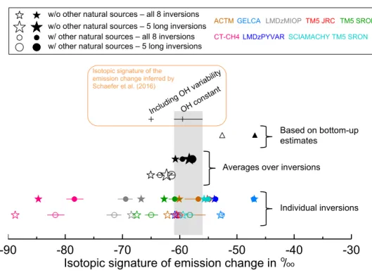
The sectorial partitioning of this emission increase be-tween the periods 2002–2006 and 2008–2012 differs from one atmospheric inversion study to another. However, all top-down studies suggest smaller changes in fossil fuel emis-sions (from oil, gas, and coal industries) compared to the mean of the bottom-up inventories included in this study. This difference is partly driven by a smaller emission change in China from the top-down studies compared to the estimate in the Emission Database for Global Atmospheric Research (EDGARv4.2) inventory, which should be revised to smaller values in a near future. We apply isotopic signatures to the emission changes estimated for individual studies based on five emission sectors and find that for six individual top-down studies (out of eight) the average isotopic signature of the emission changes is not consistent with the observed change in atmospheric13CH4. However, the partitioning in emission
change derived from the ensemble mean is consistent with this isotopic constraint. At the global scale, the top-down en-semble mean suggests that the dominant contribution to the resumed atmospheric CH4growth after 2006 comes from
mi-crobial sources (more from agriculture and waste sectors than from natural wetlands), with an uncertain but smaller contri-bution from fossil CH4emissions. In addition, a decrease in
biomass burning emissions (in agreement with the biomass burning emission databases) makes the balance of sources consistent with atmospheric13CH4observations.
In most of the top-down studies included here, OH concen-trations are considered constant over the years (seasonal vari-ations but without any inter-annual variability). As a result, the methane loss (in particular through OH oxidation) varies mainly through the change in methane concentrations and not its oxidants. For these reasons, changes in the methane loss could not be properly investigated in this study, although it may play a significant role in the recent atmospheric methane changes as briefly discussed at the end of the paper.
1 Introduction
Methane (CH4), the second most important anthropogenic
greenhouse gas in terms of radiative forcing, is highly rel-evant to mitigation policy due to its shorter lifetime and its stronger warming potential compared to carbon diox-ide. Atmospheric CH4 mole fraction has experienced a
renewed and sustained increase since 2007 after almost 10 years of stagnation (Dlugokencky et al., 2009; Rigby et al., 2008; Nisbet et al., 2014, 2016). Over 2006–2013, the atmospheric CH4growth rate was about 5 ppb yr−1
be-fore reaching 12.7 ppb yr−1in 2014 and 9.5 ppb yr−1in 2015 (NOAA monitoring network: http://www.esrl.noaa.gov/gmd/ ccgg/trends_ch4/).
The growth rate of atmospheric methane is a very accu-rate measurement of the imbalance between global sources and sinks. Methane is emitted by anthropogenic sources (livestock including enteric fermentation and manure man-agement; rice cultivation; solid waste and wastewater; fos-sil fuel production, transmission, and distribution; biomass burning) and natural sources (wetlands and other inland freshwaters, geological sources, hydrates, termites, wild an-imals). Methane is mostly destroyed in the atmosphere by hydroxyl radical (OH) oxidation (90 % of the atmospheric sink). Other sinks include destruction by atomic oxygen and chlorine, in the stratosphere and in the marine boundary layer, respectively, and upland soil sink destruction by mi-crobial methane oxidation. The changes in these sources and sinks can be investigated by different methods: bottom-up process-based models of wetland emissions (Melton et al., 2013; Bohn et al., 2015; Poulter et al., 2017), rice paddy emissions (Zhang et al. 2016), termite emissions (Sander-son, 1996; Kirschke et al., 2013, Supplement) and soil up-take (Curry, 2007), data-driven approaches for other natu-ral fluxes (e.g. Bastviken et al., 2011; Etiope, 2015), atmo-spheric chemistry climate model for methane oxidation by OH (John et al., 2012; Naik et al., 2013; Voulgarakis et al., 2013; Holmes et al., 2013), bottom-up inventories for anthro-pogenic emissions (e.g. Emission Database for Global At-mospheric Research, EDGAR; US Environmental Protection Agency, USEPA; Food and Agriculture Organization, FAO; Greenhouse Gas – Air Pollution Interactions and Syner-gies model, GAINS), observation-driven models for biomass burning emissions (e.g. Global Fire Emissions Database, GFED) and finally by atmospheric inversions, which opti-mally combine methane atmospheric observations within a chemistry transport model, and a prior knowledge of sources and sinks (inversions are also called top-down approaches, e.g. Bergamaschi et al., 2013; Houweling et al., 2014; Pison et al., 2013).
The renewed increase in atmospheric methane since 2007 has been investigated in the past recent years; atmospheric concentration-based studies suggest a mostly tropical signal, with a small contribution from the mid-latitudes and no clear change from high latitudes (Bousquet et al., 2011;
Bergam-aschi et al., 2013; Bruhwiler et al., 2014; Dlugokencky et al., 2011; Patra et al., 2016; Nisbet et al., 2016). The year 2007 was found to be a year with exceptionally high emis-sions from the Arctic (e.g. Dlugokencky et al., 2009), but it does not mean that Arctic emissions were persistently higher during the entire period 2008–2012. Attribution of the re-newed atmospheric CH4 growth to specific source and sink
processes is still being debated. Bergamaschi et al. (2013) found that anthropogenic emissions were the most impor-tant contributor to the methane growth rate increase after 2007, though smaller than in the EDGARv4.2FT2010 in-ventory. In contrast, Bousquet et al. (2011) explained the methane increases in 2007–2008 by an increase mainly in natural emissions, while Poulter et al. (2017) did not find significant trends in global wetland emissions from an en-semble of wetland models over the period 2000–2012. This flat trend over the decade is associated with large year-to-year variations (e.g. 2010–2011 in the tropics) that limit its robustness together with sensitivities to the choice of the inventory chosen to represent the wetland extent. McNor-ton et al. (2016b) using a single wetland emission model with a different wetland dynamics scheme also concluded a small increase (3 %) in wetland emissions relative to 1993– 2006. Associated with the atmospheric CH4mixing ratio
in-crease, the atmospheric δ13C-CH4 shows a continuous
de-crease since 2007 (e.g. Nisbet al., 2016), pointing towards in-creasing sources with depleted δ13C-CH4(microbial) and/or
decreasing sources with enriched δ13C-CH4(pyrogenic,
ther-mogenic). Using a box model combining δ13C-CH4and CH4
observations, two recent studies infer a dominant role of increasing microbial emissions (more depleted in 13C than thermogenic and pyrogenic sources) to explain the higher CH4 growth rate after ca. 2006. Schaefer et al. (2016)
hy-pothesised (but did not prove) that the increasing microbial source was from agriculture rather than from natural wet-lands; however, given the uncertainties in isotopic signa-tures, the evidence against wetlands is not strong. Schwi-etzke et al. (2016), using updated estimates of the source isotopic signatures (Sherwood et al., 2017) with rather nar-row uncertainty ranges also find a positive trend in micro-bial emissions. In a scenario where biomass burning emis-sions are constant over time, they inferred decreasing fossil fuel emissions, in disagreement with emission inventories. However, the global burned area is suggested to have de-creased (−1.2% yr−1)over the period 2000–2012 (Giglio et al., 2013), leading to a decrease in biomass burning emis-sions (http://www.globalfiredata.org/figures.html). In a sec-ond scenario including a 1.2 % yr−1 decrease in biomass burning emissions, Schwietzke et al. (2016) find fossil fuel emissions close to constant over time, when coal production significantly increased, mainly from China.
Atmospheric observations of ethane, a species co-emitted with methane in the oil and gas upstream sector, can be used to estimate methane emissions from this sector (e.g. Aydin et al, 2011; Wennberg et al., 2012; Nicewonger et
al., 2016). The historical record of atmospheric ethane sug-gests an increase in ethane sources until the 1980s and then a decrease driven by fossil-fuel-related emissions until the early 2000s (Aydin et al., 2011). Over the 2007-2014 period, Hausmann et al. (2016) suggested a significant increase in oil and gas methane emissions contributing to the increase in total methane emissions. However, this study, as many oth-ers, relies on emission ratios of ethane to methane, which are uncertain and may vary substantially over the years (e.g. Wunch et al., 2016), yet this potential variation over time is not well documented. The increase in methane mole frac-tions could also be due to a decrease in OH global concentra-tions (Rigby et al., 2008; Holmes et al., 2013). Although OH year-to-year variability appears to be smaller than previously thought (e.g. Montzka et al., 2011), a long-term trend can still strongly impact the atmospheric methane growth rate as a 1 % change in OH corresponds to a 5 Tg change in methane emissions (Dalsoren et al., 2009). Indeed, after an increase in OH concentrations over the period 1970–2007, Dalsoren et al. (2016) found constant OH concentrations since 2007, and Rigby et al. (2017) found a decrease in OH concentra-tions, with both results possibly contributing to the observed increase in methane growth rate and therefore limiting the required changes in methane emissions inferred by top-down studies. However, Turner et al. (2017) highlight the difficulty in disentangling the contribution in emission or sink changes when OH concentrations are weakly constrained by atmo-spheric measurements.
Using top-down approaches, an accurate attribution of changes in methane emissions per region is difficult due to the sparse coverage of surface networks (e.g. Dlugokencky et al., 2011). Satellite data offer a better coverage in some poorly sampled regions (tropics), and progress has been made in improving satellite retrievals of CH4column mole
fractions (e.g. Butz et al., 2011; Cressot et al., 2014). How-ever, the complete exploitation of remote sensing of CH4
col-umn gradients in the atmosphere to infer regional sources is still limited by relatively poor accuracy and gaps in the data, although progress has been made by moving from SCIA-MACHY (SCanning Imaging Absorption SpectroMeter for Atmospheric CHartographY) to GOSAT (Greenhouse Gases Observing Satellite; Buchwitz et al., 2015; Cressot et al., 2016). Also, the chemistry transport models often fail to cor-rectly reproduce the methane vertical gradient, especially in the stratosphere (Saad et al., 2016; Wang et al., 2016), and this misrepresentation in the models may impact the inferred surface fluxes when constrained by total column observa-tions. Furthermore, uncertainties in top-down estimates stem from uncertainties in atmospheric transport and the setup and data used in the inverse systems (Locatelli et al., 2015; Patra et al., 2011).
One approach to address inversion uncertainties is to gather an ensemble of transport models and inversions. In-stead of interpreting one single model to discuss the methane budget changes, here we take advantage of an ensemble of
published studies to extract robust changes and patterns ob-served since 2000 and in particular since the renewed in-crease after 2007. This approach allows accounting for the model-to-model uncertainties in detecting robust changes of emissions (Cressot et al., 2016). Attributing sources to sec-tors (e.g. agriculture vs. fossil) or types (e.g. microbial vs. thermogenic) using inverse systems is challenging if no ad-ditional constraints, such as isotopes, are used to separate the different methane sources, which often overlap geograph-ically. Assimilating only CH4 observations, the separation
of different sources relies only on their different seasonal-ity (e.g. rice cultivation, biomass burning, wetlands), on the signal of synoptic peaks related to regional emissions when continuous observations are available, or on distinct spatial distributions. Using isotopic information such as δ13C-CH4
brings some additional constraints on source partitioning to separate microbial vs. fossil and fire emissions, or to separate regions with a dominant source (e.g. agriculture in India ver-sus wetlands in Amazonia), but δ13C-CH4alone cannot
fur-ther separate microbial emissions between agriculture, wet-lands, termites, or freshwaters with enough confidence due to uncertainties in their close isotopic signatures.
The Global Carbon Project (GCP) has provided a collabo-rative platform for scientists from different disciplinary fields to share their individual expertise and synthesise the current understanding of the global methane budget. Following the first GCP global methane budget published by Kirschke et al. (2013) and using the same dataset as the budget update by Saunois et al. (2016) for 2000–2012, we analyse here the re-sults of an ensemble of top-down and bottom-up approaches in order to determine the robust features that could explain the variability and quasi-decadal changes in CH4growth rate
since 2000. In particular, this paper aims to highlight the most likely emission changes that could contribute to the ob-served positive trend in methane mole fractions since 2007. However, we do not address the contribution of the methane sinks during this period. Indeed, for most of the models, the soil sink is from climatological estimates and the oxidant concentration fields (OH, Cl, O1D) are assumed constant over the years. The global mean of OH concentrations was generally optimised against methyl-chloroform observations (e.g. Montzka et al., 2011), but no inter-annual variability is applied. It should be kept in mind that any OH change in the atmosphere will limit (in case of decreasing OH) or enhance (in case of increasing OH) the methane emission changes that are required to explain the observed atmospheric methane re-cent increase (e.g. Dalsoren et al., 2016; Rigby et al., 2017), as further discussed in Sect. 4.
Section 2 presents the ensemble of bottom-up and top-down approaches used in this study as well as the common data processing operated. The main results based on this en-semble are presented and discussed in Sect. 3 through global and regional assessments of the methane emission changes as well as process contributions. We discuss these results in
Sect. 4 in the context of the recent literature summarised in the introduction and draw some conclusions in Sect. 5.
2 Methods
The datasets used in this paper were those collected and pub-lished in The Global Methane Budget 2000–2012 (Saunois et al., 2016). The decadal budget is publicly available at http://doi.org/10.3334/CDIAC/Global_Methane_Budget_ 2016_V1.1 and on the Global Carbon Project website. Here, we only describe the main characteristics of the datasets and the reader may refer to the aforementioned detailed paper. The datasets include an ensemble of global top-down ap-proaches as well as bottom-up estimates of the sources and sinks of methane.
2.1 Top-down studies
The top-down estimates of methane sources and sinks are provided by eight global inverse systems, which optimally combine a prior knowledge of fluxes with atmospheric ob-servations, both with their associated uncertainties, into a chemistry transport model in order to infer methane sources and sinks at specific spatial and temporal scales. Eight in-verse systems have provided a total of 30 inversions over 2000–2012 or shorter periods (Table 1). The longest time series of optimised methane fluxes are provided by inver-sions using surface in situ measurements (15). Some surface-based inversions were provided over time periods shorter than 10 years (7). Satellite-based inversions (8) provide es-timates over shorter time periods (2003–2012 with SCIA-MACHY; from June 2009 to 2012 using TANSO/GOSAT). As a result, the discussion presented in this paper will be essentially based on surface-based inversions as GOSAT of-fers too short a time series and SCIAMACHY is associ-ated with large systematic errors that need ad hoc correc-tions (e.g. Bergamaschi et al., 2013). Most of the inverse systems estimate the total net methane emission fluxes at the surface (i.e. surface sources minus soil sinks), although some systems solve for a few individual source categories (Table 1). In order to speak in terms of emissions, each in-version provided its associated soil sink fluxes that have been added to the associated net methane fluxes to obtain esti-mates of surface sources. Saunois et al. (2016) attempted to separate top-down emissions into five categories: wetland emissions, other natural emissions, emissions from agricul-ture and waste handling, biomass burning emissions (includ-ing agricultural fires), and fossil-fuel-related emissions. To obtain these individual estimates from those inversions only solving for the net flux, the prior contribution of each source category was used to split the posterior total sources into in-dividual contributions.
Table 1. List of the top-down estimates included in this paper.
Model Institution Observation used Time Flux solved Number of References
period inversions
Carbon Tracker-CH4 NOAA Surface stations 2000–2009 10 terrestrial sources
and oceanic source
1 Bruhwiler et al. (2014) LMDZ-MIOP LSCE-CEA Surface stations 1990–2013 Wetlands, biomass burning, and
other natural, anthropogenic sources
10 Pison et al. (2013)
LMDZ-PYVAR LSCE-CEA Surface stations 2006–2012 Net source 6 Locatelli et al. (2015)
LMDZ-PYVAR LSCE-CEA GOSAT satellite 2010–2013 3
TM5 SRON Surface stations 2003–2010 Net source 1 Houweling et al. (2014)
TM5 SRON GOSAT satellite 2009–2012 2
TM5 SRON SCIAMACHY satellite 2003–2010 1
TM5 EC-JRC Surface stations 2000–2012 Wetlands, rice, biomass
burn-ing, and all remaining sources
1 Bergamaschi et al. (2013); Alexe et al. (2015)
TM5 EC-JRC GOSAT satellite 2010–2012 1
GELCA NIES Surface stations 2000–2012 Natural (wetland, rice, termite), anthropogenic (excluding rice), biomass burning, soil sink
1 Ishizawa et al. (2016); Zhuravlev et al. (2013)
ACTM JAMSTEC Surface stations 2002–2012 Net source 1 Patra et al. (2016)
NIES-TM NIES Surface stations 2010–2012 Biomass burning,
anthropogenic emissions (excluding rice paddies), and all natural sources (including rice paddies)
1 Kim et al. (2011); Saito et al. (2016)
NIES-TM NIES GOSAT satellite 2010–2012 1
2.2 Bottom-up studies
The bottom-up approaches gather inventories for anthro-pogenic emissions (agriculture and waste handling, fossil-fuel-related emissions, biomass burning emissions), land sur-face models (wetland emissions), and diverse data-driven approaches (e.g, local measurement upscaling) for emis-sions from fresh waters and geological sources (Table 2). Anthropogenic emissions are from the Emission Database for Global Atmospheric Research (EDGARv4.1, 2010; EDGARV4.2FT2010, 2013), the United States Environmen-tal Protection Agency, USEPA (USEPA, 2006, 2012), and the Greenhouse Gas – Air Pollution Interactions and Syner-gies (GAINS) model developed by the International Institute for Applied Systems Analysis (IIASA; Höglund-Isaksson, 2012). They report methane emissions from the following major sources: livestock (enteric fermentation and manure management); rice cultivation; solid waste and wastewater; fossil fuel production, transmission, and distribution. How-ever, they differ in the level of detail by sector, by country, and by the emission factors used for some specific sectors and countries (Höglund-Isaksson et al., 2015). The Food and Agriculture Organization (FAO) FAOSTAT emissions dataset (FAOSTAT, 2017a, b) contains estimates of agricultural and biomass burning emissions (Tubiello et al., 2013, 2015). Biomass burning emissions are also taken from the Global Fire Emissions Database (version GFED3, van der Werf et al., 2010, and version GFED4s, Giglio et al., 2013; Ran-derson et al., 2012), the Fire Inventory from NCAR (FINN; Wiedinmyer et al., 2011), and the Global Fire Assimilation System (GFAS, Kaiser et al., 2012). For wetlands, we use the results of 11 land surface models driven by the same dynamic
flooded area extent dataset from remote sensing (Schroeder et al., 2015) over the 2000–2012 period. These models differ mainly in their parameterisations of CH4flux per unit area
in response to climate and biotic factors (Poulter et al., 2017; Saunois et al., 2016).
2.3 Data analysis
The top-down and bottom-up estimates are gathered sepa-rately and compared as two ensembles for anthropogenic, biomass burning, and wetland emissions. For the bottom-up approaches, the category called “other natural” encompasses emissions from termites, wild animals, lakes, oceans, and natural geological seepage (Saunois et al., 2016). However, for most of these sources, limited information is available re-garding their spatiotemporal distributions. Most of the inver-sions used here include termite and ocean emisinver-sions in their prior fluxes; some also include geological emissions (Ta-ble S1 in the Supplement). However, the emission distribu-tions used by the inversions as prior fluxes are climatological and do not include any inter-annual variability. Geological methane emissions have played a role in past climate changes (Etiope et al., 2008). There is no study on decadal changes in geological CH4 emissions on continental and global scales,
although it is known that they may increase or decrease in relation to seismic activity and variations of groundwater hy-drostatic pressure (i.e. aquifer depletion).
Ocean emissions have been revised downward recently (Saunois et al., 2016). Inter-decadal changes in lake fluxes cannot be made in reliable ways because of the data scarcity and lack of validated models (Saunois et al., 2016). As a result of a lack of quantified evidences, variations of lakes,
Table 2. List of the bottom-up studies included in this paper.
Bottom-up models Contribution Time period Gridded References
and inventories (resolution)
EDGAR4.2 FT2010 Fossil fuels, agriculture and waste, biofuel
2000–2010 (yearly) X EDGARv4.2FT2010 (2013); Olivier et al. (2012) EDGARv4.2FT2012 Total anthropogenic 2000–2012 (yearly) EDGARv4.2FT2012 (2014);
Olivier and
Janssens-Maenhout (2014); Rogelj et al. (2014) EDGARv4.2EXT Fossil fuels, agriculture
and waste, biofuel
1990–2013 (yearly) Based on EDGARv4.1 (EDGARv4.1, 2010); this study
USEPA Fossil fuels, agriculture and waste, biofuel,
1990–2030 (10-year interval, interpolated in this study)
USEPA (2006, 2011, 2012)
IIASA GAINS ECLIPSE Fossil fuels, agriculture and waste, biofuel
1990–2050 (5-year interval, interpolated in this study) X Höglund-Isaksson (2012); Klimont et al. (2017)
FAOSTAT Agriculture, biomass burning Agriculture: 1961–2012 Biomass burning: 1990–2014 Tubiello et al. (2013, 2015)
GFEDv3 Biomass burning 1997–2011 X van der Werf et al. (2010)
GFEDv4s Biomass burning 1997-2014 X Giglio et al. (2013)
GFASv1.0 Biomass burning 2000-2013 X Kaiser et al. (2012)
FINNv1 Biomass burning 2003–2014 X Wiedinmyer et al. (2011)
CLM 4.5 Natural wetlands 2000–2012 X Riley et al. (2011);
Xu et al. (2016)
CTEM Natural wetlands 2000-2012 X Melton and Arora (2016)
DLEM Natural wetlands 2000–2012 X Tian et al. (2010, 2015)
JULES Natural wetlands 2000–2012 X Hayman et al. (2014)
LPJ-MPI Natural wetlands 2000–2012 X Kleinen et al. (2012)
LPJ-wsl Natural wetlands 2000–2012 X Hodson et al. (2011)
LPX-Bern Natural wetlands 2000–2012 X Spahni et al. (2011)
ORCHIDEE Natural wetlands 2000–2012 X Ringeval et al. (2011)
SDGVM Natural wetlands 2000–2012 X Woodward and Lomas (2004);
Cao et al. (1996) TRIPLEX-GHG Natural wetlands 2000–2012 X Zhu et al. (2014, 2015)
VISIT Natural wetlands 2000–2012 X Ito and Inatomi (2012)
oceans, and geological sources are ignored in our bottom-up analysis. However, it should be noted that possible varia-tions of these sources are accounted for in the top-down ap-proaches in the “other natural” category.
Some results are presented as box plots showing the 25, 50, and 75 % percentiles. The whiskers show minimum and maximum values excluding outliers, which are shown as stars. The mean values are plotted as “+” symbols on the box plot. The values reported in the text are the mean (XX), minimum (YY), and maximum (ZZ) values as XX [YY– ZZ]. Some estimates rely on few studies so that meaning-ful 1σ values cannot be computed. To consider that methane
changes are positive or negative for a time-period (e.g. Figs. 3 and 4 in Sect. 3), we consider that the change is robustly pos-itive or negative when both the first and third quartiles are positive or negative, respectively.
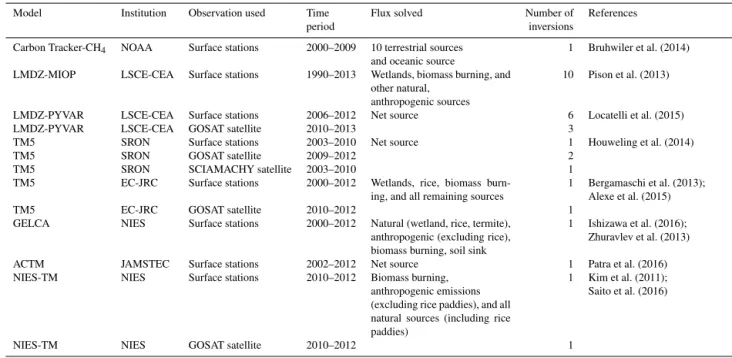
Figure 1. Evolution of the global methane cycle since 2000. (a) Observed atmospheric mixing ratios (ppb) as synthesised for four different surface networks with a global coverage (NOAA, AGAGE, CSIRO, UCI). (b) Global growth rate computed from (a) in ppb yr−1. The 12-month running mean of (c) the annual global emission (Tg CH4yr−1)and (d) the annual global emission anomaly (Tg ‘CH4yr−1)inferred by the ensemble of inversions.
3 Results
3.1 Global methane variations in 2000-2012 3.1.1 Atmospheric changes
The global average methane mole fractions are from four in situ atmospheric observation networks: the Earth System Re-search Laboratory from the US National Oceanic and Atmo-spheric Administration (NOAA ESRL; Dlugokencky et al., 1994), the Advanced Global Atmospheric Gases Experiment (AGAGE; Rigby et al., 2008), the Commonwealth Scien-tific and Industrial Research Organisation (CSIRO, Francey et al., 1999), and the University of California, Irvine (UCI;
Simpson et al., 2012). The four networks show a consistent evolution of the globally averaged methane mole fractions (Fig. 1a). The methane mole fractions refer here to the same NOAA2004A CH4 reference scale. The different sampling
sites used to compute the global average and the sampling frequency may explain the observed differences between networks. Indeed, the UCI network samples atmospheric methane in the Pacific Ocean between 71◦N and 47◦S us-ing flasks durus-ing specific campaign periods, while other net-works use both continuous and flask measurements world-wide. During the first half of the 2000s, the methane mole fraction remained relatively stable (1770–1785 ppb), with small positive growth rate until 2007 (0.6 ± 0.1 ppb yr−1,
Years Emission anomaly (Tg CH 4 yr -1 ) 2002 2006 2010 -40 -20 0 20
40 (a) Global total sources
-20 -10 0 10
20 (c) Mid-latitude total sources
2002 2006 2010
-40 -20 0 20
40 (e) Global anthropogenic sources
(b) Tropical total sources
(d) Boreal total sources
2002 2006 2010
(f) Global natural sources
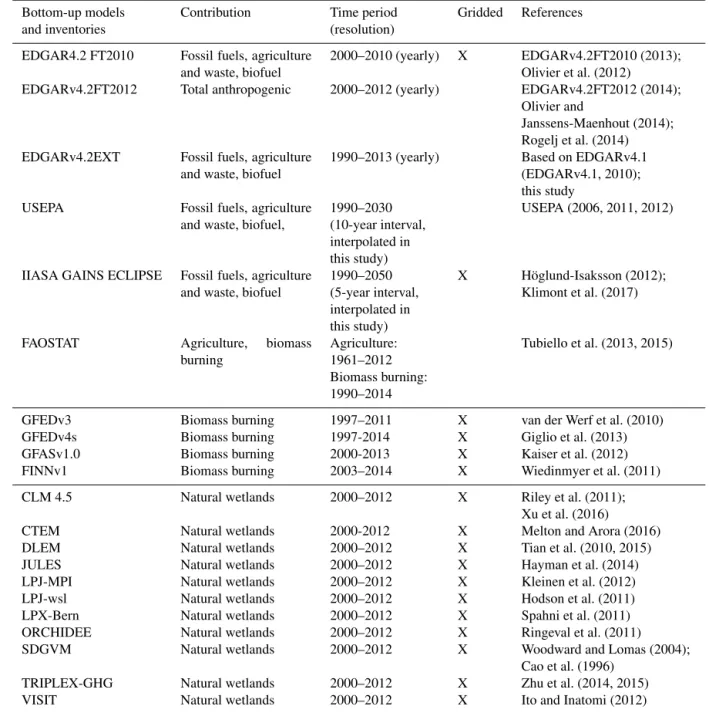
Figure 2. The 12-month running mean of annual methane emission anomalies (in Tg CH4yr−1)inferred by the ensemble of inversions
(mean as the solid line and min–max range as the shaded area) in grey for (a) global, (b) tropical, (c) mid-latitudes, and (d) boreal total sources; in blue for (e) global anthropogenic sources; and in green for (f) natural sources. The solid and dotted black lines represent the mean and min–max range (respectively) of the bottom-up estimates: anthropogenic inventories in (e) and ensemble of wetland models in (f). The vertical scale is divided by 2 for the mid-latitude and boreal regions.
Years Emission anomaly (Tg CH 4 yr -1) 2002 2004 2006 2008 2010 2012 -20 -10 0 10 20
(a) Total anthrop Biomass burning Fossil fuel Agriculture & waste
2002 2004 2006 2008 2010 2012 -20 -10 0 10 20
Agriculture & waste + fossil fuel (b)
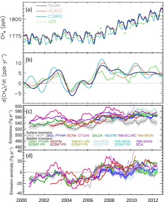
Figure 3. The 12-month running mean of global annual methane anthropogenic emission anomalies (Tg CH4yr−1)inferred by the
ensemble of inversions (only mean values of the ensemble are rep-resented) for (a) total anthropogenic, biomass burning, fossil fuel, and agriculture and waste sources. On the (b) panel, total anthro-pogenic, and agriculture and waste source anomalies are recalled on top of the sum of the anomalies from agriculture, waste, and fossil fuels sources.
Fig. 1b). Since 2007, methane atmospheric mole fraction rose again, reaching 1820 ppb in 2012. A mean growth rate of 5.2 ± 0.2 ppb yr−1over the period 2008–2012 is observed (Fig. 1b).
3.1.2 Global emission changes in individual inversions
As found in several studies (e.g. Bousquet et al., 2006), the flux anomaly (see Supplement, Sect. 2) from top-down in-versions (Fig. 1d) is found more robust than the total source estimate when comparing different inversions (Fig. 1c). The mean range between the inverse estimates of total global emissions (Fig. 1c) is of 35 Tg CH4yr−1(14 to 54 over the
years and inversions reported here); this means that the un-certainty in the total annual global methane emissions in-ferred by top-down approaches is about 6 % (35 Tg CH4yr−1
over 550 Tg CH4yr−1). It is to be noted that this rather good
agreement between these estimates is linked with the asso-ciated rather small range of global sinks. Indeed, most in-versions use similar methyl chloroform (MCF)-constrained OH fields and temperature fields. The three top-down stud-ies spanning 2000 to 2012 (Table 1) show an increase of 15 to 33 Tg CH4yr−1 between 2000 and 2012 (Fig. 1d).
Despite the increase in global methane emissions being of the order of magnitude of the range between the mod-els, flux anomalies clearly show that all individual inver-sions infer an increase in methane emisinver-sions over the period 2000–2012 (Fig. 1d). The inversions using satellite obser-vations included here mainly use GOSAT retrievals (start-ing from mid-2009), and only one inversion is constrained with SCIAMACHY column methane mole fractions (from 2003 but ending in 2012, dashed lines in Fig. 1d). On aver-age, satellite-based inversions infer higher annual emissions than surface-based inversions (+12 Tg CH4yr−1higher over
−10 0 10 20 30 40 Methane emissions (Tg CH 4 .yr − 1 ) Global 9 0 ° S − 3 0 ° N 3 0 − 6 0 ° N 6 0 − 9 0 ° N
Central N. America Trop. S. America Temp. S. America
Northern Africa Southern Africa
India
South East Asia
Oceania
Contiguous USA
Europe China
Temp. cent. Eurasia & Japan
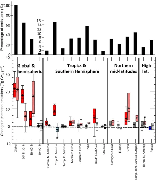
Boreal N. America Russia Global & hemispheric Tropics & Southern Hemisphere Northern mid-latitudes lat. High 100 80 60 40 20 0 16 14 12 10 8 6 4 2 Pe rce nt ag e of emi ssi on s (% ) Change in me th an e emi ssi on s (T g C H4 yr -1)
Figure 4. Top: contribution to the global methane emissions by region (in %, based on the mean top-down estimates over 2003–2012 from Saunois et al., 2016). Bottom: changes in methane emissions over 2002–2006 and 2008–2012 at global, hemispheric, and regional scales in TgCH4yr−1. Red box plots indicate a significant positive contribution to emission changes (first and third quartiles above zero), blue
box plots indicate a significant negative contribution to emission changes (first and third quartiles below zero), and grey box plots indicate not-significant emission changes. Dark coloured boxes are for top-down (five long inversions) and light coloured for bottom-up approaches (see text for details). The median is indicated inside each box plot (see Sect. 2). Mean values, reported in the text, are represented with “+” symbols. Outliers are represented with stars. (Note: the bottom-up approaches that provide country estimates – and not maps, USEPA and FAOSTAT – have not been processed to provide hemispheric values. As a result the ensemble used for the three hemispheric regions differs from the ensemble used for the global and regional estimates.)
2010–2012) as previously shown in Saunois et al. (2016) and Locatelli et al. (2015). Also, it is worth noting that the ensem-ble of top-down results shows emissions that are consistently lower in 2009 and higher in 2008 and 2010 (Figs. 1c and S1 in the Supplement).
3.1.3 Year-to-year changes
When averaging the anomalies in global emissions over the inversions, we find a difference of 22 [5–37] Tg CH4
be-tween the yearly averages for 2000 and 2012 (Fig. 2a). Over
the period 2000–2012, the variations in emission anomalies reveal both year-to-year changes and a positive long-term trend. Year-to-year changes are found to be the largest in the tropics: up to ±15 Tg CH4yr−1 (Fig. 2b), with a
neg-ative anomaly in 2004–2006 and a positive anomaly after 2007 visible in all inversions except one (Fig. 1d). Com-pared with the tropical signal, mid-latitude emissions ex-hibit smaller anomalies (mean anomaly mostly below 5 Tg CH4yr−1, except around 2005) but contribute a rather sharp
increase in 2006–2008, marking a transition between the pe-riod 2002–2006 and the pepe-riod 2008–2012 at the global scale
(Fig. 2a and c). The boreal regions do not contribute signif-icantly to year-to-year changes, except in 2007, as already noted in several studies (Dlugokencky et al., 2009; Bousquet et al., 2011).
When splitting global methane emissions into anthro-pogenic and natural emissions at the global scale (Fig. 2e and f, respectively), both of these two general categories show significant year-to-year changes. As natural and an-thropogenic emissions occur concurrently in several regions, top-down approaches have difficulty in separating their con-tribution. Therefore the year-to-year variability allocated to anthropogenic emissions from inversions may be an arte-fact of our separation method (see Sect. 2) and/or reflect the larger variability between studies compared to natural emissions. However, some of the anthropogenic methane sources are sensitive to climate, such as rice cultivation or biomass burning, and also, to a lesser extent, enteric fermen-tation and waste management. Fossil fuel exploifermen-tation can also be sensitive to rapid economic changes, and meteoro-logical variability may impact the fuel demand for heating and cooling systems. However, anthropogenic emissions re-ported by bottom-studies (black line on Fig. 2e) show much fewer year-to-year changes than inferred by top-down in-versions (blue line of Fig. 2e). China coal production rose faster from 2002 until 2011, when its production started to stabilise or even decline (IEA, 2016). This last period is characterised by major reorganisations in the Chinese coal industry, including evolution from many small gassy mines to fewer mines with better safety and emission control. The global natural gas production steadily increased over time de-spite a short drop in production in 2009 following the eco-nomic crisis (IEA, 2016). The bottom-up inventories do re-flect some of this variation, such as in 2009 when gas and oil methane emissions slightly decreased (EDGARv4.2FT2010 and EDGARv4.2EXT, Fig. S7). Methane emissions from agriculture and waste are continuously growing in the bottom-up inventories at the global scale. The observed activ-ity data underlying the emissions from agriculture estimated in this study, as reported by countries to FAO via the FAO-STAT database (FAO, 2017a, b), exhibit inter-annual vari-abilities that partly explain the variability in methane emis-sions discussed herein. Livestock methane emisemis-sions from the Americas (mainly South America) increased mainly be-tween 2000 and 2004 and remained stable afterwards (esti-mated by FAOSTAT, Fig. S12). Additionally, Asian (India, China, and South and East Asia) livestock emissions mainly increased between 2004 and 2008 and also remained rather stable afterwards. In contrast, livestock emissions in Africa increased continuously over the full period. These continen-tal variations translate into global livestock emissions in-creasing continuously over the full period, though at a slower rate after 2008 (Fig. S13). Overall, these anthropogenic emis-sions exhibit more semi-decadal to decadal evolutions (see below) than year-to-year changes as found in top-down in-versions.
For natural sources, the mean anomaly of the top-down ensemble suggests year-to-year changes ranging ±10 Tg CH4yr−1, which is lower than but in phase with the total
source mean anomaly. The mean anomaly of global natural sources inferred by top-down studies is negative around 2005 and positive around 2007 (Fig. 2f). The year-to-year varia-tion in wetland emissions inferred from land surface models is of the same order of magnitude but out of phase compared to the ensemble mean top-down estimates (Fig. 2f). How-ever, some individual top-down approaches suggest anoma-lies smaller than or of different sign than the mean of the ensemble (Fig. S2). Also, some land surface models show anomalies in better agreement with the top-down ensemble mean in 2000–2006 (Fig. S11). The 2009 (2010) negative (positive) anomaly in wetland emissions is common to all land surface models (Fig. S11) and is the result of varia-tions in flooded areas (mainly in the tropics) and in tempera-ture (mainly in boreal regions) (Poulter et al., 2017). Overall, from the contradictory results from top-down and bottom-up approaches, it is difficult to draw any robust conclusions on the year-to-year variations in natural methane emissions over the period 2000–2012.
3.1.4 Decadal trend
The mean anomaly of the inversion estimates shows a positive linear trend in global emissions of +2.2 ± 0.2 Tg CH4yr−2 over 2000–2012 Fig. 2a). It originates mainly
from increasing tropical emissions (+1.6 ± 0.1 Tg CH4yr−2,
Fig. 2b) with a smaller contribution from the mid-latitudes (+0.6 ± 0.1 Tg CH4yr−2, Fig. 2c). The positive global trend
is explained mostly by an increase in anthropogenic emis-sions, as separated in inversions (+2.0 ± 0.1 Tg CH4yr−2,
Fig. 2e). This represents an increase of about 26 Tg CH4
in the annual anthropogenic emissions between 2000 and 2012, casting serious doubt on the bottom-up methane in-ventories for anthropogenic emissions, showing an increase in anthropogenic emissions of +55 [45–73] Tg CH4between
2000 and 2012, with USEPA and GAINS inventories at the lower end and EDGARv4.2FT2012 at the higher end of the range. This possible overestimation of the recent anthro-pogenic emissions increase by inventories has already been suggested in individual studies (e.g. Patra et al., 2011; Berga-maschi et al., 2013; Bruhwiler et al., 2014; Thompson et al., 2015; Peng et al., 2016; Saunois et al., 2016) and is con-firmed in this study as a robust feature. Splitting the anthro-pogenic sources into the components identified in the method section, the trend in anthropogenic emissions from top-down studies mainly originates from the agriculture and waste sec-tor (+1.2 ± 0.1 Tg CH4yr−2, Fig. 3a). Adding the fossil fuel
emission trend almost matches the global trend of anthro-pogenic emissions (Fig. 3b). It should be noted here that the individual inversions all suggest constant to increasing emis-sions from agriculture and waste handling (Fig. S3), while some suggest constant to decreasing emissions from fossil
fuel use and production (Fig. S4). The latter result seems surprising in view of large increases in coal production dur-ing 2000–2012, especially in China. However, this recent pe-riod is characterised by major reorganisations in the Chinese coal industry, including evolution from many small gassy mines to fewer mines with better safety and emission con-trol. The trend in biomass burning emissions is small but barely significant between 2000 and 2012 (−0.05 ± 0.05 Tg CH4yr−2, Fig. 3). This result is consistent with the GFED
dataset (both versions 3 and 4s) for which no significant trend was found over this 13-year period. However, between 2002 and 2010, a significant negative trend of −0.5 ± 0.1 Tg CH4yr−2 is found for biomass burning, both from the
top-down approaches (Fig. S5) and the GFED3 and GFED4s in-ventory (Fig. S10); this corresponds to dry years in the trop-ics. Although it should be noted that almost all inversions use GFED3 in their prior fluxes (Table S1) and therefore are not independent from the bottom-up estimates Over the 13-year period, the wetland emissions in the inversions show a small positive trend (+0.2 ± 0.1 Tg CH4yr−2)about twice
as large as the trends of emissions from land surface models but within the range of uncertainty (+0.1 ± 0.1 Tg CH4yr−2,
Poulter et al., 2017). As stated previously, the wetland emis-sions from some land surface models disagree with the en-semble mean of land surface models (Fig. S11).
3.1.5 Quasi-decadal changes in the period 2000–2012 According to Fig. 2a, the period 2000–2012 is split into two parts – before 2006 and after 2008. Neither a significant nor a systematic trend in the global total sources (among the in-versions of Fig. 1d) is observed before 2006, likewise after 2008 (see Fig. S6 for individual calculated trends); although large year-to-year variations are visible. Before 2006, anthro-pogenic emissions show a positive trend of +2.4 ± 0.2 Tg CH4yr−2, compensated for by decreasing natural emissions
(−2.4 ± 0.2 Tg CH4yr−2; calculated from Fig. 2e and f),
which explains the rather stable global total emissions. Bous-quet et al. (2006) discussed such compensation between 1999 and 2003. The behaviour of the top-down ensemble mean is consistent with a decrease in microbial emissions in 2000– 2006, especially in the Northern Hemisphere as suggested by Kai et al. (2011) using13CH4observations. However, Levin
et al. (2012) showed that the isotopic data selection might bias this result, as they found no such decrease when using background site measurements. Indeed, some individual top-down studies still suggest constant emissions from both nat-ural and anthropogenic sources (Figs. S2, S3 and S4) over that period as found by Levin et al. (2012) or Schwietzke et al. (2016), with both also using13CH4observations. The
different trends in anthropogenic and natural methane emis-sions among the inveremis-sions highlight the difficulties of the top-down approach in separating natural from anthropogenic emissions and also its dependence on prior emissions. All inversions are based on EDGAR inventory (most of them
us-ing EDGARv4.2 version, Table S1). However, the estimated posterior anthropogenic emissions can significantly deviate from this common prior estimate. Similarly, inversions based on the same prior wetland fluxes do not systematically in-fer the same variations in methane total and natural emis-sions. These different increments from the prior fluxes are constrained by atmospheric observations and qualitatively in-dicate that inversions can depart from prior estimates. Con-trary to the ensemble mean of inversions, the land surface models gathered in this study show on average a small posi-tive trend (+0.7 ± 0.1 Tg CH4yr−2)during 2000–2006
(cal-culated from Fig. 2f), with some exceptions in individuals models (Fig. S11). Recently, Schaefer et al. (2016), based on isotopic data, suggested that diminishing thermogenic emis-sions caused the early 2000s plateau without ruling out vari-ations in the OH sink. However, another scenario explaining the plateau could combine both constant total sources and sinks. Over 2000–2006, no decrease in thermogenic emis-sions is found in any of the inveremis-sions included in our study (Fig. S4). Even using time-constant prior emissions for fossil fuels in the inversions results in robustly inferring increasing fossil fuel emissions after 2000, although lower than when using inter-annually varying prior estimates from inventories (e.g. Bergamaschi et al., 2013).
All inversions show increasing emissions in the second half of the period, after 2006. For the period 2006–2012, most inversions show a significant positive trend (below 5 Tg CH4yr−2), within 2σ uncertainty for most of the available
inversions (see Fig. S6). Most of this positive trend is ex-plained by the years 2006 and 2007, due to both natural and anthropogenic emissions, but appears to be highly sen-sitive to the period of estimation (Fig. S6). Between 2008 and 2012, neither the total anthropogenic nor the total natu-ral sources present a significant trend, leading to rather stable global total methane emissions (Fig. 2e and f). Overall, these results suggest that emissions shifted between 2006 and 2008 rather than continuously increasing after 2006. The require-ment of a step change in the emissions will be further dis-cussed in Sect. 4. Because of this, in the following section, we analyse in more details the emission changes between two time periods: 2002–2006 and 2008–2012 at global and re-gional scales.
3.2 The methane emission changes between 2002–2006 and 2008–2012
3.2.1 Global and hemispheric changes inferred by top-down inversions
Integrating all inversions covering at least 3 years over each 5-year period, the global methane emissions are estimated at 545 [530–563] Tg CH4yr−1 on average over 2002–2006
and at 569 [546–581] Tg CH4yr−1 over 2008–2012. It is
worth noting some inversions do not contribute to both pe-riods, leading to different ensembles being used to compute
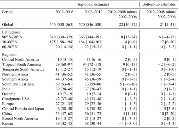
Table 3. Average methane emissions over 2002–2006 and 2008–2012 at the global, latitudinal, and regional scales in Tg CH4yr−1, and
differences between the periods 2008–2012 and 2002–2006 from the top-down and the bottom-up approaches. Uncertainties are reported as a [min–max] range of reported studies. Differences of 1 Tg CH4yr−1in the totals can occur due to rounding errors. A minimum of 3 years
was required to calculate the average value over the 5-year periods, and then the difference between the two periods was calculated for each approach. This means that 5 inversions are used to produce these values.
Top-down estimates Bottom-up estimates Period 2002–2006 2008–2012 2012–2008 minus 2012–2008 minus 2002–2006 2002–2006 Global 546 [530–563] 570 [546–580] 22 [16–32] 21 [5–41] Latitudinal 90◦S–30◦N 349 [330–379] 363 [344–391] 18 [13–24] 6 [−4–13] 30–60◦N 175 [158–194] 184 [164–203] 4 [0–9] 17 [6–30] 60–90◦N 20 [14–24] 22 [15–31] 0 [−1–1] 0 [−3–3] Regional
Central North America 10 [3–15] 11 [6–16] 2 [0–5] 0 [0–1]
Tropical South America 79 [60–97] 94 [72–118] 9 [6–13] −2 [−6–2] Temperate South America 17 [12–27] 15 [12–19] 0 [−1–1] 0 [−1–0]
Northern Africa 41 [36–52] 41 [36–55] 2 [0–5] 2 [0–5]
Southern Africa 44 [37–54] 45 [36–59] 0 [−3–3] 1 [−2–4]
South and East Asia 69 [53–81] 73 [59–86] 5 [−6–10] 1 [−3–4]
India 39 [28–45] 37 [26–47] 0 [−1–1] 2 [1–3]
Oceania 10 [7–19] 10 [7–14] 0 [0–1] 0 [−1–1]
Contiguous USA 42 [37–48] 42 [33–48] 1 [−2–3] 2 [−1–4]
Europe 27 [21–35] 29 [22–36] 1 [−1–3] −2 [−2–2]
Central Eurasia and Japan 46 [38–50] 48 [38–58] 1 [−1–6] 5 [2–6]
China 53 [47–62] 56 [41–73] 4 [1–11] 10 [2–20]
Boreal North America 19 [13–27] 21 [15–27] 0 [−3–3] 2 [0–5]
Russia 39 [32–45] 38 [30–44] −1 [−3–0] 0 [−4–3]
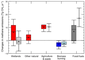
Table 4. Mean values of the emission change (in Tg CH4yr−1)
be-tween 2002–2006 and 2008–2012 inferred from the top-down and bottom-up approaches for the five general categories.
Top-down Bottom-up Wetlands 6 [−4–16] −1 [−8–7] Agriculture and waste 10 [7–12] 10 [7–13] Fossil fuels 7 [−2–16] 17 [11–25] Biomass burning −3 [−7–0] −2 [−5–0]
Other natural 2 [−2–7] –
these estimates. Despite the different ensembles (seven stud-ies for 2002–2006 and 10 studstud-ies for 2008–2012), the esti-mate ranges for both periods are similar. Keeping only the five surface-based inversions covering both periods leads to 542 [530–554] Tg CH4yr−1on average over 2002–2006 and
563 [546–573] Tg CH4yr−1 over 2008–2012, showing
re-markably consistent values with the ensemble of the top-down studies and also not showing significant impact in the emission differences between the two time periods (see Ta-ble S3).
The emission changes between the period 2002–2006 and the period 2008–2012 have been calculated for inversions covering at least 3 years over both 5-year periods (5 inver-sions) at global, hemispheric, and regional scales (Fig. 4). The regions are the same as in Saunois et al. (2016). The re-gion denoted as “ 90◦S–30◦N” is referred to as the tropics
despite the southern mid-latitudes (mainly from Oceania and temperate South America) included in this region. However, since the extra-tropical Southern Hemisphere contributes less than 8% to the emissions from the “90◦S–30◦N” region, the region primarily represents the tropics.
The global emission increase of +22 [16–32] Tg CH4yr−1
is mostly tropical (+18 [13–24] Tg CH4yr−1, or ∼ 80 % of
the global increase). The northern mid-latitudes only con-tribute an increase of +4 [0–9] Tg CH4yr−1, while the
high-latitudes (above 60◦N) contribution is not significant. How-ever, most inversions rely on surface observations, which poorly represent the tropical continents, as previously no-ticed by a previous study (e.g. Bousquet et al., 2011). As a result, this tropical signal may partly be an artefact of inver-sions attributing emission changes to unconstrained regions. Also, the absence of a significant contribution from the Arc-tic region means that ArcArc-tic changes are below the detection
limit of inversions. Indeed, the northern high latitudes emit-ted about 20 [14–24] Tg CH4yr−1 of methane over 2002–
2006 and 22 [15–31] Tg CH4yr−1over 2008–2012 (Table 3),
but keeping inversions covering at least 3 years over each 5-year period leads to a null emission change in boreal regions. The geographical partition of the increase in emissions be-tween 2000–2006 and 2008–2012 inferred here is in agree-ment with Bergamaschi et al. (2013), who found that 50– 85 % of the 16–20 Tg CH4emission increase between 2007–
2010 and 2003–2005 came from the tropics and the rest from the Northern Hemisphere mid-latitudes. Houweling et al. (2014) inferred an increase of 27–35 Tg CH4yr−1
be-tween the 2-year periods before and after July 2006. The ensemble of inversions gathered in this study infer a consis-tent increase of 30 [20–41] Tg CH4yr−1between the same
two periods. The derived increase is highly sensitive to the choice of the starting and ending dates of the time period. The study of Patra et al. (2016) based on six inversions found an increase of 19–36 Tg CH4yr−1in global methane
emis-sions between 2002–2006 and 2008–2012, which is consis-tent with our results.
3.2.2 Regional changes inferred by top-down inversions At the regional scale, top-down approaches infer different emission changes both in amplitude and in sign. These dis-crepancies are due to transport errors in the models and to differences in inverse setups and can lead to several tens of per cent differences in the regional estimates of methane emissions (e.g. Locatelli et al., 2013). Indeed, the recent study of Cressot et al. (2016) showed that, while global and hemispheric emission changes could be detected with con-fidence by the top-down approaches using satellite obser-vations, their regional attribution is less certain. Thus, it is particularly critical for regional emissions to rely on several inversions, as done in this study, before drawing any robust conclusion. In most of the top-down results (Fig. 4), the trop-ical contribution to the global emission increase originates mainly in tropical South America (+9 [6–13] Tg CH4yr−1)
and South and East Asia (+5 [−6–10] Tg CH4yr−1). Central
North America (+2 [0–5] Tg CH4yr−1)and northern Africa
(+2 [0–5] Tg CH4yr−1)contribute less to the tropical
emis-sion increase. The sign of the contribution from South and East Asia is positive in most studies (e.g. Houweling et al., 2014), although some studies infer decreasing emission in this region. The disagreement between inversions could re-sult from the lack of measurement stations to constrain the fluxes in Asia (some have appeared inland India and China but only in the last years, Lin et al., 2017), and also from the rapid up-lift of the compounds emitted at the surface to the free troposphere by convection in this region, leading to sur-face observations missing information on local fluxes (e.g. Lin et al., 2015).
In the northern mid-latitudes a positive contribution is in-ferred for China (+4 [1–11] Tg CH4yr−1)and Central
Eura-sia and Japan (+1 [−1–6] Tg CH4yr−1). Also, temperate
North America does not contribute significantly to the sion changes. Contrary to a large increase in the US emis-sions suggested by Turner et al. (2016), none of the inver-sions detect, at least prior to 2013, an increase in methane emissions possible due to increasing shale gas exploitation in the US. Bruhwiler et al. (2017) highlight the difficulty of deriving trends on relatively short term due to, in particular, inter-annual variability in transport.
The inversions agree that emissions changes remained lim-ited in the Arctic region but do not agree on the sign of the emission change over the high northern latitudes, especially over boreal North America; however, they show a consis-tent small emission decrease in Russia. This lack of agree-ment between inversions over the boreal regions highlights the weak sensitivity of inversions in these regions where no or little methane emission changes are found to have oc-curred over the last decade. Changes in wetland emissions associated with sea ice retreat in the Arctic are probably only a few Tg between the 1980s and the 2000s (Parmen-tier et al., 2015). Also, decreasing methane emissions in sub-Arctic areas that were drying and cooling over 2003–2011 have offset increasing methane emissions in a wetting Arctic and warming summer (Watts et al., 2014). Permafrost thaw-ing may have caused additional methane production under-ground (Christensen et al., 2004), but changes in the methane flux to the atmosphere have not been detected by continu-ous atmospheric stations around the Arctic, despite a small increase in late autumn–early winter in methane emission from Arctic tundra (Sweeney et al., 2016). However, unin-tentional double counting of emissions from different water systems (wetlands, rivers, lakes) may lead to Artic emission growth in the bottom-up studies when little or none exists (Thornton et al., 2016). The detectability of possibly increas-ing methane emissions from the Arctic seems possible today based on the continuous monitoring of the Arctic atmosphere at a few but key stations (e.g. Berchet et al., 2016; Thonat et al., 2017), but this surface network remains fragile in the long term and would be more robust with additional constraints such as those that will be provided in 2021 by the active satel-lite mission MERLIN (Pierangello et al., 2016; Kiemle et al., 2014).
3.2.3 Emission changes in bottom-up studies
The top-down approaches use bottom-up estimates as a priori values. For anthropogenic emissions, most of them use the EDGARv4.2FT2010 inventory and GFED3 emis-sion estimates for biomass burning. Their source of a pri-ori information differs more for the contribution from nat-ural wetlands, geological emissions, and termite sources (Table S1). Here we gathered an ensemble of bottom-up estimates for the changes in methane emissions between 2000–2006 and 2008–2012, combining anthropogenic in-ventories (EDGARv4.2FT2010, USEPA, and GAINS), five
biomass burning emission estimates (GFED3, GFED4s, FINN, GFAS, and FAOSTAT), and wetland emissions from 11 land surface models (see Sect. 2 for the details and Saunois et al., 2016 and Poulter et al., 2017). As previously stated, other natural methane emissions (termites, geological, inland waters) are assumed in these model studies to not con-tribute significantly to the change between 2000–2006 and 2008–2012, because no quantitative indications are available on such changes and because at least some of these sources are less climate sensitive than wetlands.
The bottom-up estimate of the global emission change between the periods 2000–2006 and 2008–2012 (+21 [5– 41] Tg CH4yr−1, Fig. 4) is comparable but possesses a
larger spread than top-down estimates (+22 [16–32] Tg CH4yr−1). Also, the hemispheric breakdown of the change
reveals discrepancies between top-down and bottom-up es-timates. The bottom-up approaches suggest a much higher increase in emissions in the mid-latitudes (+17 [6–30] Tg CH4yr−1)than inversions and a smaller increase in the
trop-ics (+6 [−4–13] Tg CH4yr−1). The main regions where
bottom-up and top-down estimates of emission changes dif-fer are tropical South America, South and East Asia, China, USA, and central Eurasia and Japan.
While top-down studies indicate a dominant increase be-tween 2000–2006 and 2008–2012 in tropical South America (+9 [6–13] Tg CH4yr−1), the bottom-up estimates (based on
an ensemble of 11 land surface models and anthropogenic in-ventories), in contrast, indicate a small decrease (−2 [−6–2] Tg CH4yr−1)over the same period (Fig. 4). The decrease
in tropical South American emissions found in the bottom-up studies results from decreasing emissions from wetlands (about −2.5 Tg CH4yr−1, mostly due to a reduction in
trop-ical wetland extent, as constrained by the common inventory used by all models, see Poulter et al., 2017) and biomass burning (about −0.7 Tg CH4yr−1), partly compensated for
by a small increase in anthropogenic emissions (about 1 Tg CH4yr−1, mainly from agriculture and waste). Most of the
top-down studies infer a decrease in biomass burning emis-sions over this region, exceeding the decrease in a priori emissions from GFED3. Thus, the main discrepancy between top-down and bottom-up is due to microbial emissions from natural wetlands (about 4 Tg CH4yr−1on average),
agricul-ture, and waste (about 2 Tg CH4yr−1on average) over
trop-ical South America.
The emission increase in South and East Asia for the bottom-up estimates (2 Tg CH4yr−1) results from a 4 Tg
CH4yr−1 increase (from agriculture and waste for half of
it, fossil fuel for one-third, and wetland for the remainder) offset by a decrease in biomass burning emissions (−2 [−4– 0] Tg CH4yr−1). The inversions suggest a higher increase in
South and East Asia compared to this 2 Tg CH4yr−1, mainly
due to higher increases in wetland and agriculture and waste sources, with the biomass burning decrease and the fossil fuel increase being similar in the inversions compared to the in-ventories. − −10 0 10 20 30 Emission differences (TgCH 4 .yr − 1) C ha ng es in me th an e emi ssi on s (T g C H4 yr -1)
Wetlands Other natural Agriculture
& waste Biomass burning Fossi l fuels Figure 5. Changes in methane emissions between 2002–2006 and 2008–2012 in Tg CH4yr−1for the five source types. Red box plots
indicate a significant positive contribution to emission changes (first and third quartiles above zero), blue box plots indicate a significant negative contribution to emission changes (first and third quartiles below zero), and grey box plots indicate non-significant emission changes. Dark (light) coloured boxes are for top-down (bottom-up) approaches (see text for details). The median is indicated inside each box plot (see Methods, Sect. 2). Mean values, reported in the text, are represented with “+” symbols.
In tropical South America and South and East Asia, wet-lands and agriculture and waste emissions may both occur in the same or neighbouring model pixels, making the parti-tioning difficult for the top-down approaches. Also, these two regions lack surface measurement sites, so the inverse sys-tems are less constrained by the observations. However, the SCIAMACHY-based inversion from Houweling et al. (2014) also infers increasing methane emissions over tropical South America between 2002–2006 and 2008–2012. Further stud-ies based on satellite data or additional regional surface ob-servations (e.g. Basso et al., 2016; Xin et al., 2015) would be needed to better assess methane emissions (and their changes) in these under-sampled regions.
For China, bottom-up approaches suggest a +10 [2–20] Tg CH4yr−1emission increase between 2002–2006 and 2008–
2012, i.e. a trend of about 1.7 Tg CH4yr−2 (considering a
10 Tg yr−1increase over 2004–2010), which is much larger than the top-down estimates. The magnitude of the Chinese emission increase varies among emission inventories and es-sentially appears to be driven by an increase in anthropogenic emissions (fossil fuel and agriculture and waste emissions). Anthropogenic emission inventories indicate that Chinese emissions increased at a rate of 0.6 Tg CH4yr−2in USEPA,
3.1 Tg yr−2in EDGARv4.2, and 1.5 Tg CH4yr−2in GAINS
between 2000 and 2012. The increase rate in EDGARv4.2 is too strong compared to a recent bottom-up study that suggests a 1.3 Tg CH4yr−2 increase in Chinese methane
emissions over 2000–2010 (Peng et al., 2016). The revised EDGAR inventory v4.3.2 (not officially released when we