HAL Id: hal-01644270
https://hal.inria.fr/hal-01644270v2
Submitted on 19 Feb 2019
HAL is a multi-disciplinary open access
archive for the deposit and dissemination of sci-entific research documents, whether they are pub-lished or not. The documents may come from teaching and research institutions in France or abroad, or from public or private research centers.
L’archive ouverte pluridisciplinaire HAL, est destinée au dépôt et à la diffusion de documents scientifiques de niveau recherche, publiés ou non, émanant des établissements d’enseignement et de recherche français ou étrangers, des laboratoires publics ou privés.
Analytic expressions of the solutions of
advection-diffusion problems in 1D with discontinuous
coefficients
Antoine Lejay, Lionel Lenôtre, Géraldine Pichot
To cite this version:
Antoine Lejay, Lionel Lenôtre, Géraldine Pichot. Analytic expressions of the solutions of advection-diffusion problems in 1D with discontinuous coefficients. SIAM Journal on Applied Mathematics, Society for Industrial and Applied Mathematics, 2019, 79 (5), pp.1823-1849. �10.1137/18M1164500�. �hal-01644270v2�
Analytic expressions of the solutions of
advection-diffusion problems in 1D with
discontinuous coefficients
Antoine Lejay
*,
Lionel Lenôtre
†,
Géraldine Pichot
‡November 18, 2017
Abstract
In this article, we provide a method to compute analytic expressions of the resolvent kernel of differential operators of the diffusion type with discontinuous coefficients in one dimension. Then we apply it when the coefficients are piecewise constant. We also perform the Laplace inversion of the resolvent kernel to obtain expressions of the transition density functions or fundamental solutions. We show how these explicit formula are useful to simulate advection-diffusion problems using particle tracking techniques.
Keywords: advection diffusion problems; resolvent kernels; transition density functions; discontinuous coefficients; particle tracking techniques
1
Introduction
We consider linear second-order parabolic operators 𝒜𝐵𝑥,(𝑎,𝜌,𝑏) with domain Dom(𝒜𝐵𝑥,(𝑎,𝜌,𝑏)) such as:
𝒜𝐵
𝑥,(𝑎,𝜌,𝑏)𝑓 (𝑥) :=
1
2𝜌(𝑥)𝜕𝑥(𝑎(𝑥)𝜕𝑥𝑓 (𝑥)) + 𝑏(𝑥)𝜕𝑥𝑓 (𝑥),
with 𝑎 and 𝑏 possibly discontinuous. The coefficients 𝑎 and 𝑏 may be discontinuous at different points and/or may have several points of discontinuities.
*Université de Lorraine, IECL, UMR 7502, Vandœuvre-lès-Nancy, F-54500, France
CNRS, IECL, UMR 7502, Vandœuvre-lès-Nancy, F-54500, France Inria, Villers-lès-Nancy, F-54600, France
Contact: IECL, BP 70238, F-54506 Vandœuvre-lès-Nancy CEDEX, France. Email: [email protected]
†CMAP, Ecole Polytechnique, France
Contact: CMAP UMR 7641 Ecole Polytechnique CNRS, Route de Saclay, 91128 Palaiseau Cedex France, Email: [email protected]
‡Inria Paris, 2 rue Simone Iff, 75012 Paris
Université Paris-Est, CERMICS (ENPC), 77455 Marne-la-Vallée 2, France Contact: Inria Paris, 2 rue Simone Iff, CS 42112, 75589 Paris Cedex 12 Email: [email protected]
We are interested in deriving analytic expressions of the resolvent kernels (or of its Laplace inversion, the so-called transition density functions) of such operators and to use these analytic ex-pressions in the context of particle tracking methods [13, 14, 43]. These analytic exex-pressions may also provide other very interestings results as asymptotics in long time [49] and short time [10], various quantities such as option prices in finance [46], solution of inverse problems [28] or understanding of the underlying equations and their spectral properties [25, 26].
Due to the discontinuities of 𝑎 and/or 𝑏, the derivation of analytic expressions of the resolvent kernel of (𝒜𝐵𝑥,(𝑎,𝜌,𝑏), Dom(𝒜𝐵
𝑥,(𝑎,𝜌,𝑏))) requires special methods. Commonly, these analytic
ex-pressions are derived using probabilistic methods or arguments [2, 6, 17, 23, 58]. However, the derivation is quite heavy and sometimes cumbersome. Other approaches, described in [25, 26], in the same spirit of the method proposed in this paper, consider only the case 𝑏 = 0.
Our first contribution consists in proposing a general computation method which provides explicit, closed form formula of the resolvent kernel when both 𝑎 and 𝑏 are discontinuous; extending the previous results we cited right above. It also generalizes the so-called method of imageswhich was only usable when the symmetries in the coefficients allow it [60]. The method we propose is more universal and systematic than the existing ones with probabilistic arguments which tends to treat the problems case by case. In the situation where 𝑎 and 𝑏 are piecewise constant, we show how to end up, through a simple change of variable, to the study of a Skew Brownian motion [39] with drift (called the drifted Skew Brownian motion).
Then we are interested in using the analytic expression of the resolvent kernel of 𝒜𝐵
𝑥,(𝑎,𝜌,𝑏) in the
context of solving advection-diffusion problems with a particle tracking technique. We consider the classical advection-diffusion operator:
ℒ𝐵
𝑥𝑓 (𝑡, 𝑥) :=
1
2𝜕𝑥(𝑎(𝑥)𝜕𝑥𝑓 (𝑥)) + 𝑏(𝑥)𝜕𝑥𝑓 (𝑥),
with domain Dom(ℒ𝐵𝑥). On purpose, we take the same coefficient 𝑎 and 𝑏 as the ones in the expression of 𝒜𝐵𝑥,(𝑎,𝜌,𝑏).
The coefficient 𝑎 is classically called the diffusivity coefficient and the coefficient 𝑏 the drift. The operator (ℒ𝐵𝑥, Dom(ℒ𝐵
𝑥)) is encountered in many applications: in (with only a few references)
geophysics for soil [12, 29, 32, 52, 57], air [56] and ocean [54]; astrophysics [61]; molecular dynamics [8]; population ecology [9, 36]; finance [11, 24, 59]. The discontinuities come generally from the medium, which contains permeable or semi-permeable barriers. For example, in ther-modynamics or electronics, the materials are built with layers possessing different conductivity in order to reach some effective behavior. Similarly, in population ecology, different intertwined habitats has to be dealt with while studying the concentration of insects’ population.
When 𝑎 and 𝑏 are discontinuous, the Gaussian approximation is no longer valid [27, 32] and special particle tracking schemes have to be designed. In the litterature, most of the already proposed schemes take 𝑏 = 0 [5, 16, 17, 29, 40, 43, 47, 53, 57]. In [15, 42] (random walk based methods) — which are not sensitive with regard to the values of the drifts — as well as in [13, 17] (exact simulation techniques), either 𝑎 or 𝑏 is discontinuous but not both.
Our second contribution consists in emphasizing the connection between the two operators 𝒜𝐵
𝑥,(𝑎,1,𝑏) and ℒ 𝐵
𝑥. In fact, when the coefficients 𝑎 and 𝑏 are the same, the two operators ℒ𝐵𝑥
and 𝒜𝐵𝑥,(𝑎,1,𝑏) (𝜌 = 1) differ only because they are defined with different ambient spaces. We demonstrate rigorously that it is possible to compute the resolvent kernel of ℒ𝐵𝑥 with the one of 𝒜𝐵
𝑥,(𝑎,1,𝑏). The resolvent of 𝒜 𝐵
𝑥,(𝑎,1,𝑏) is itself obtained using the computation method presented in
at different points of discontinuities. Additionnally, we show that computing the resolvent kernel of 𝒜𝐵𝑥,(𝑎,1,𝑏) in the case of one interface of discontinuity in an infinite domain is sufficient to design a general particle tracking algorithm in the general case of advection-diffusion problems with multiple interfaces of discontinuities. This last result is obtained by using the definition of interface layersaround the discontinuities as proposed in [44] together with the Markov property of the stochastic process associated to ℒ𝐵
𝑥.
Outline. In Section 2, we recall a few results regarding second-order differential operators of the diffusion type and their resolvent equations whose solutions are the Green functions: their factorized forms and their minimal pairs in particular. In Section 3, we provide our computation method which provide analytic closed form expression of the resolvent kernel (Green function). In Section 4, we treat in full detail the situation where the diffusivity and the advective term (or drift) are piecewise constant. We show how it reduces, through a simple change of variable, to the study of the drifted Skew Brownian motion. Using inverse Laplace transforms, we derive some explicit expressions for the transition density function (or the fundamental solution) for some particular situations. In Sections 5 and 6, we show that this general methodology is useful for solving advection-diffusion problems with particle tracking techniques. Section 5 details the case of one interface of discontinuity and Section 6 proposes a general algorithm to handle the case of multiple interfaces.
2
Operators and their resolvents
In this section, we present the second-order differential operators we consider as well as some of its main properties that will be used subsequently in Section 3. More precisely, we consider a large-class of operators which depends on 3 functions and whose ambient space of the space of bounded, continuous functions.
For some constants 0 < 𝑐 ≤ 𝐶, we define
c:= {𝑎 : R → R+measurable | 𝑐 ≤ 𝑎(𝑥) ≤ 𝐶, ∀𝑥 ∈ R}, (2.1)
b:= {𝑏 : R → R measurable | |𝑏(𝑥)| ≤ 𝐶, ∀𝑥 ∈ R} (2.2) and M := {(𝑎, 𝜌, 𝑏) : R → R3| 𝑎, 𝜌 ∈ c, 𝑏 ∈ b}.
We denote by 𝒞(𝐼, 𝐽 ) the space of continuous functions from 𝐼 ⊂ R to a state space 𝐽 . Denote by 𝒞0the class of continuous functions vanishing at infinities equipped with the uniform norm ‖·‖∞.
It is indeed a Banach space.
To each (𝑎, 𝜌, 𝑏) ∈ M, we associate the second-order differential operator whose existence is asserted by Proposition 2.1 below:
𝒜𝐵 𝑥,(𝑎,𝜌,𝑏)𝑓 (𝑥) := 1 2𝜌(𝑥)𝜕𝑥(𝑎(𝑥)𝜕𝑥𝑓 (𝑥)) + 𝑏(𝑥)𝜕𝑥𝑓 (𝑥), Dom(𝒜𝐵𝑥,(𝑎,𝜌,𝑏)) = {𝑓 ∈ 𝒞0| 𝒜𝐵𝑥,(𝑎,𝜌,𝑏) ∈ 𝒞0}.
2.1
Factorized forms
Following the approach of W. Feller [22], we look at a factorized form of 𝒜𝐵𝑥,(𝑎,𝜌,𝑏). This factorized form is particularly suitable for providing an explicit expression of resolvent kernel.
Definition 2.1. For a function 𝑓 ∈ 𝒞0, the differentiability of𝑓 at 𝑥 with respect to a continuous
and increasing function𝐺 : R → R is defined as
D𝐺𝑥𝑓 (𝑥) = lim
𝑦↘𝑥
𝑓 (𝑦) − 𝑓 (𝑥) 𝐺(𝑦) − 𝐺(𝑥) when the limit exists.
Remark2.1. When 𝐺(𝑥) = 𝑥, the differentiability is just the classical differentiability. Hence, we write 𝜕𝑥in spite of D𝐺:𝑥↦→𝑥𝑥 .
Proposition 2.1. Let (𝑎, 𝜌, 𝑏) ∈ M. The differential operator (𝒜𝐵
𝑥,(𝑎,𝜌,𝑏), Dom(𝒜 𝐵
𝑥,(𝑎,𝜌,𝑏))) is well
defined and can be factorized as:
𝒜𝐵𝑥,(𝑎,𝜌,𝑏) = 1 2D 𝑀 𝑥 D 𝑆 𝑥,
where𝑆 is the scale function, 𝑀 is the speed measure with
𝑆(𝑥) = ∫︁ 𝑥 0 𝜅(𝑦) 𝑎(𝑦) d𝑦 and 𝑀 (𝑥) = ∫︁ 𝑥 0 1 𝜌(𝑦)𝜅(𝑦)d𝑦, (2.3) 𝑠(𝑥) = 𝜅(𝑥) 𝑎(𝑥), 𝑚(𝑥) = 1 𝜅(𝑥)𝜌(𝑥), ℎ(𝑥) = ∫︁ 𝑥 0 2𝑏(𝑦) 𝑎(𝑦)𝜌(𝑦)d𝑦 and 𝜅(𝑥) = 𝑒 −ℎ(𝑥). (2.4)
Remark2.2. Using Definition 2.1,
D𝑆𝑥𝑓 (𝑥) = 𝑠(𝑥)−1𝜕𝑥𝑓 (𝑥) and D𝑀𝑥 𝑓 (𝑥) = 𝑚(𝑥) −1
𝜕𝑥𝑓 (𝑥).
Proof. For the above functions 𝑆 and 𝑀 , let us define Ω := 12D𝑀
𝑥 D𝑆𝑥 with domain
Dom(Ω) := {𝑓 ∈ 𝒞0| Ω𝑓 ∈ 𝒞0}, (2.5)
= {𝑓 ∈ 𝒞0| ∀𝜆 > 0, ∃𝑤 ∈ 𝒞0 s.t. (𝜆 − Ω)𝑓 = 𝑤}. (2.6)
The existence of (Ω, Dom(Ω)) as well as the equivalence between (2.5) and (2.6) follows from classical results of W. Feller [18–21].
Now let Φ be a continuous, increasing function with Φ(0) = 0 and 𝑓 ∈ 𝒞0 be such that
𝑓 ∘ Φ ∈ Dom(𝒜𝐵𝑥,(𝑎,𝜌,𝑏)) (which we assume to be not empty in a first time). Then,
𝒜𝐵 𝑥,(𝑎,𝜌,𝑏)(𝑓 ∘ Φ)(𝑥) = (︂ 𝜌(𝑥) 2 𝑎(𝑥)Φ ′′ (𝑥) + 𝑏(𝑥)Φ′(𝑥) )︂ 𝜕𝑧𝑓 (Φ(𝑥)) +𝜌(𝑥) 2 Φ ′ (𝑥)𝜕𝑥(𝑎(𝑥)(Φ ′ )−1(𝑥)𝜕𝑥𝑓 (Φ(𝑥))).
In the meanwhile, choosing Φ(𝑥) such that Φ(0) = 0 and Φ′(𝑥) = 𝜅(𝑥) = exp(−ℎ(𝑥)) where ℎ and 𝜅 given by (2.4) ensures that
𝜌(𝑥) 2 𝑎(𝑥)Φ ′′ (𝑥) + 𝑏(𝑥)Φ′(𝑥) = 0 and 𝒜𝐵 𝑥,(𝑎,𝜌,𝑏)(𝑓 ∘ Φ)(𝑥) = 𝜌(𝑥) 2 Φ ′ (𝑥)𝜕𝑥 (︂ 𝑎(𝑥) (︂ 1 Φ′ (𝑥)𝜕𝑥(𝑓 ∘ Φ)(𝑥) )︂)︂ = 1 2𝑚(𝑥) −1 𝜕𝑥(𝑠(𝑥)−1𝜕𝑥(𝑓 ∘ Φ)(𝑥)) = 1 2D 𝑀 𝑥 D𝑆𝑥(𝑓 ∘ Φ)(𝑥) = Ω(𝑓 ∘ Φ)(𝑥).
Hence, 𝑓 ∘ Φ ∈ Dom(Ω) and then (Ω, Dom(Ω)) extends (𝒜𝐵𝑥,(𝑎,𝜌,𝑏), Dom(𝒜𝐵𝑥,(𝑎,𝜌,𝑏))).
Finally, performing the same reasoning by starting with Ω instead of 𝒜𝐵𝑥,(𝑎,𝜌,𝑏) shows the equality between the two operators. Moreover, it proves that Dom(𝒜𝐵𝑥,(𝑎,𝜌,𝑏)) ̸= ∅ since Dom(Ω) ̸= ∅. The operator (𝒜𝐵𝑥,(𝑎,𝜌,𝑏), Dom(𝒜𝐵
𝑥,(𝑎,𝜌,𝑏))) is therefore well defined.
In dimension 1, solving 𝒜𝐵
𝑥,(𝑎,𝜌,𝑏)𝑓 = 𝑔 with 𝑔 ∈ 𝒞0 is equivalent to solve a Sturm-Liouville
problem. A first application of using the factorized form is then to give some continuity properties of 𝑓 and D𝑆𝑥𝑓 .
Lemma 2.1. Let 𝑓 ∈ Dom(𝒜𝐵
𝑥,(𝑎,𝜌,𝑏)) with (𝑎, 𝜌, 𝑏) ∈ M. Then 𝑓 is continuous, differentiable
andD𝑆𝑥𝑓 is itself continuous.
Proof. From the definition of the domain of 𝒜𝐵𝑥,(𝑎,𝜌,𝑏)(see (2.5)), the problem (𝜆−𝒜𝐵𝑥,(𝑎,𝜌,𝑏))𝑓 (𝑥) = 𝑤(𝑥) is a Sturm-Liouville problem that may be transformed into solving a first-order differential equation in (𝑓, D𝑆𝑥𝑓 ), which are then necessarily (absolutely) continuous.
We now recall the definition of the resolvent kernel, which we aim at computing here. Definition 2.2 (Resolvent kernel). The resolvent kernel of 𝒜𝐵
𝑥,(𝑎,𝜌,𝑏) is a function(𝜆, 𝑥, 𝑦) ∈
R+× R × R ↦→ r𝒜𝐵
𝑥,(𝑎,𝜌,𝑏)(𝜆; 𝑥, 𝑦) such that the family (𝐺𝜆)𝜆>0of linear operators defined by
𝐺𝜆𝑓 (𝑥) :=
∫︁
R
r𝒜𝐵
𝑥,(𝑎,𝜌,𝑏)(𝜆; 𝑥, 𝑦)𝑓 (𝑦) d𝑦, ∀𝑓 ∈ 𝒞0 (2.7)
is the resolvent of(𝒜𝐵𝑥,(𝑎,𝜌,𝑏), Dom(𝒜𝐵𝑥,(𝑎,𝜌,𝑏))). This means that 𝐺𝜆 = (𝜆 − 𝒜𝐵𝑥,(𝑎,𝜌,𝑏))
−1 in 𝒞 0.
Formally,
(𝜆 − 𝒜𝐵𝑥,(𝑎,𝜌,𝑏))r𝒜𝐵
𝑥,(𝑎,𝜌,𝑏)(𝜆; 𝑥, 𝑦) = 𝛿𝑦(𝑥).
2.2
Minimal pair and their continuity
With the factorized form of the operator comes two particular families of functions. These functions play a central role to compute the resolvent kernel.
Proposition 2.2 ( [21, Theorem 6.1]). There exist two families {𝜑(𝜆; ·)}𝜆>0and{𝜓(𝜆; ·)}𝜆>0of
continuous, positive functions fromR to R such that
(𝜆 − 𝒜𝐵𝑥,(𝑎,𝜌,𝑏))𝑢(𝜆; 𝑥) = 0, ∀𝑥 ∈ R, 𝜆 > 0, for 𝑢 = 𝜑 or 𝜓, 𝜑(𝜆; 0) = 𝜓(𝜆; 0) = 1, 𝜑 is decreasing from +∞ to 0,
𝜓 is valued increasing from 0 to +∞.
The pair(𝜑, 𝜓) is called the minimal pair.
Being unbounded, 𝜑(𝜆; ·) and 𝜓(𝜆; ·) do not belong to Dom(𝒜𝐵𝑥,(𝑎,𝜌,𝑏)). The proof of the next lemma is similar to the one of Lemma 2.1.
Lemma 2.2. For each 𝜆 > 0, the functions 𝜑(𝜆; ·), 𝜓(𝜆; ·), D𝑆𝑥𝜑(𝜆; ·) and D𝑆𝑥𝜓(𝜆; ·) are contin-uous onR.
3
Resolvent kernel of knotted operators
Using the notations of (2.1)-(2.2), we set
C:= c ∩ 𝒞(R, R) and B := b ∩ 𝒞(R, R) as well as
H:= {(𝑎, 𝜌, 𝑏) : R → R3| 𝑎, 𝜌 ∈ C, 𝑏 ∈ B} ⊂ M.
Notation3.1. For two functions 𝜉−and 𝜉+from R to R𝑑(𝑑 ≥ 1), we define their knotting as
𝜉− ◁▷ 𝜉+: R −→ R𝑑,
𝑥 ↦−→ 𝜉−(𝑥)1𝑥<0+ 𝜉+(𝑥)1𝑥≥0.
For a space F of continous functions from R to R𝑑, we write F◁▷:= {𝑓− ◁▷ 𝑓+| 𝑓−, 𝑓+∈ F}.
The problem of knotting operators consists in finding suitable conditions at the interface when “gluing” the diffusion processes they generate (See e.g. [37]). In our case, we have a natural interpretation of the transmission condition but we are interested in finding analytic expressions. Remark3.1. We choose to knot functions at 0 for convenience of the presentation. Actually, everything we propose in this paper does not require 𝑎 and 𝑏 to be knotted at the same point nor to have only one single point of knotting.
We now restrict our attention to coefficients which are obtained by knotting simpler ones. Hypothesis3.1. We consider two families (𝑎±, 𝜌±, 𝑏±) in H from which we define
(𝑎, 𝜌, 𝑏) = (𝑎−, 𝜌−, 𝑏−) ◁▷ (𝑎+, 𝜌+, 𝑏+) ∈ H◁▷.
Notation3.2. To (𝑎±, 𝜌±, 𝑏±) ∈ H we associate the corresponding operators 𝒜𝐵𝑥,(𝑎±,𝜌±,𝑏±), scales
functions 𝑆±, speed measures 𝑀± with density 𝑚±, the minimal pairs (𝜑±, 𝜓±), and so on.
Remark3.2. With (2.4) and (2.3), the scale measure 𝑆 and the density 𝑚 of speed measure 𝑀 of 𝒜𝐵 𝑥,(𝑎,𝜌,𝑏) satisfy 𝑆 = 𝑆− ◁▷ 𝑆+and 𝑚 = 𝑚− ◁▷ 𝑚+. Notation3.3. We define 𝑔(𝜆; 𝑥, 𝑦) := r𝒜𝐵 𝑥,(𝑎,𝜌,𝑏)(𝜆; 𝑥, 𝑦) 𝑚(𝑦) for (𝜆, 𝑥, 𝑦) ∈ R+× R × R. (3.1)
As it will be seen below in (3.7), this kernel 𝑔(𝜆; 𝑥, 𝑦) is symmetric in (𝑥, 𝑦).
We now give a characterization of the resolvent kernel from which we deduce our analytic conditions. Let us recall the formal expression in Definition 2.2. With Lemma 2.1, continuity conditions are imposed at 0, which are translated in (3.3)-(3.4) below. The effect of the Dirac mass in Definition 2.2 is rewritten as a condition on the jump of a flow: See (3.6) below. Condition (3.2) can be solved locally using the minimal pairs as they form a local basis for solutions.
Proposition 3.1. Let (𝑎, 𝜌, 𝑏) ∈ H◁▷as in Hypothesis 3.1. The kernel𝑔(𝜆; 𝑥, 𝑦) given by (3.7) associated to(𝒜𝐵 𝑥,(𝑎,𝜌,𝑏), Dom(𝒜 𝐵 𝑥,(𝑎,𝜌,𝑏))) solves: (𝜆 − 𝒜𝐵𝑥,(𝑎,𝜌,𝑏))𝑔(𝜆; 𝑥, 𝑦) = 0, 𝑥, 𝑦 ∈ R, 𝑥 ̸∈ {𝑦, 0}, (3.2) 𝑔(𝜆; 0−, 𝑦) = 𝑔(𝜆; 0+, 𝑦), 𝑦 ̸= 0, (3.3) 𝑔(𝜆; 𝑦−, 𝑦) = 𝑔(𝜆; 𝑦+, 𝑦), 𝑦 ̸= 0, (3.4) D𝑆− 𝑥 𝑔(𝜆; 0−, 𝑦) = D 𝑆+ 𝑥 𝑔(𝜆; 0+, 𝑦), 𝑦 ̸= 0, (3.5) {︃ D𝑆− 𝑥 𝑔(𝜆; 𝑦−, 𝑦) − D𝑆𝑥−𝑔(𝜆; 𝑦+, 𝑦) = 2, if 𝑦 < 0, D𝑆+ 𝑥 𝑔(𝜆; 𝑦−, 𝑦) − D𝑆𝑥+𝑔(𝜆; 𝑦+, 𝑦) = 2, if 𝑦 > 0. (3.6)
Notation3.4. We define the Wronskian of two suitable functions 𝑓 and 𝑔 as Wr[𝑓, 𝑔](𝑥) := 𝑓 (𝑥)D𝑆
𝑥𝑔(𝑥) − 𝑔(𝑥)D𝑆𝑥𝑓 (𝑥).
Proof. From [21, §7, p. 475] or [30], using the minimal pair (𝜑, 𝜓) of 𝒜𝐵𝑥,(𝑎,𝜌,𝑏), 𝑔(𝜆; 𝑥, 𝑦) may be written as: 𝑔(𝜆; 𝑥, 𝑦) = 2 𝑊 {︃ 𝜓(𝜆; 𝑥)𝜑(𝜆; 𝑦) if 𝑥 < 𝑦, 𝜑(𝜆; 𝑥)𝜓(𝜆; 𝑦) if 𝑥 ≥ 𝑦 (3.7) with 𝑊 = Wr[𝜑(𝜆; ·), 𝜓(𝜆; ·)](𝑥) (this function is constant in 𝑥). Eq. (3.2) follows from (3.7). From Lemma 2.2, 𝑢(𝜆; ·) and D𝑆𝑢(𝜆; ·) are continuous for 𝑢 = 𝜑, 𝜓. Thus 𝑥 ↦→ 𝑔(𝜆; 𝑥, 𝑦) is continuous, which leads to (3.3). In addition, 𝑥 ↦→ D𝑆
𝑥𝑔(𝜆; 𝑥, 𝑦) is continuous when 𝑥 ̸= 0. As
𝑆 = 𝑆−◁▷ 𝑆+, this leads to (3.5).
Let us assume that 𝑦 > 0. When 𝑥 ≥ 𝑦, D𝑆+
𝑥 𝑔(𝜆; 𝑦 + ℎ, 𝑦) =
2 𝑊D
𝑆+
𝑥 𝜑(𝜆; 𝑦 + ℎ)𝜓(𝜆; 𝑦). Using
the expression of 𝑊 , for ℎ > 0, 𝜓(𝜆; 𝑦 + ℎ)D𝑆+ 𝑥 𝜑(𝜆; 𝑦 + ℎ) = −𝑊 + 𝜑(𝜆; 𝑦 + ℎ)D 𝑆+ 𝑥 𝜓(𝜆; 𝑦 + ℎ). Thus, D𝑆+ 𝑥 𝑔(𝜆; 𝑦 + ℎ, 𝑦) = 2 𝑊 (︀−𝑊 + 𝜑(𝜆; 𝑦 + ℎ)D 𝑆+ 𝑥 𝜓(𝜆; 𝑦 + ℎ) )︀ 𝜓(𝜆; 𝑦) 𝜓(𝜆; 𝑦 + ℎ). (3.8) Similarly, when 𝑥 < 𝑦, D𝑆+ 𝑥 𝑔(𝜆; 𝑦 − ℎ, 𝑦) = 2 𝑊D 𝑆+
𝑥 𝜓(𝜆; 𝑦 − ℎ)𝜑(𝜆; 𝑦). Using the expression
of 𝑊 , for a ℎ > 0 yields D𝑆+ 𝑥 𝑔(𝜆; 𝑦 − ℎ, 𝑦) = 2 𝑊 (︀𝑊 + 𝜓(𝜆; 𝑦 − ℎ)D 𝑆+ 𝑥 𝜑(𝜆; 𝑦 − ℎ) )︀ 𝜑(𝜆; 𝑦) 𝜑(𝜆; 𝑦 − ℎ). (3.9) Summing the two expressions (3.8) and (3.9) and using the continuity of 𝜑, 𝜓, D𝑆+
𝑥 𝜓 and D𝑆𝑥+𝜑
at 𝑦 yields (3.6) for the case 𝑦 > 0 as ℎ → 0.
For the case 𝑦 < 0, use the same arguments with the operator D𝑆−
𝑥 .
Hypothesis3.2. For (𝑎, 𝜌, 𝑏) = (𝑎−, 𝜌−, 𝑏−) ◁▷ (𝑎+, 𝜌+, 𝑏+) as in Hypothesis 3.1, we assume
that the minimal pairs (𝜑±, 𝜓±) associated to (𝑎±, 𝜌±, 𝑏±) are known.
This is the case when the coefficients (𝑎±, 𝜌±, 𝑏±) are constant as well as for many other cases [7].
Notation3.5. We consider two suitable continuous functions 𝑢 and 𝑣 The Wronskian (negative side) of 𝑢 and 𝑣 is defined by
WrN[𝑢, 𝑣](𝑥) := 𝑢(𝑥)D𝑆− 𝑥 𝑣(𝑥) − 𝑣(𝑥)D 𝑆− 𝑥 𝑢(𝑥), 𝑥 < 0, WrP[𝑢, 𝑣](𝑥) := 𝑢(𝑥)D𝑆+ 𝑥 𝑣(𝑥) − 𝑣(𝑥)D 𝑆+ 𝑥 𝑢(𝑥), 𝑥 ≥ 0, WrSNP[𝑢, 𝑣](0) := 𝑢(0)D𝑆+ 𝑥 𝑣(0) − 𝑣(0)D 𝑆− 𝑥 𝑢(0), and WrSPN[𝑢, 𝑣](0) := 𝑢(0)D𝑆− 𝑥 𝑣(0) − 𝑣(0)D 𝑆+ 𝑥 𝑢(0).
Theorem 3.1. Assume Hypothesis 3.2. Let𝑔(𝜆; 𝑥, 𝑦) be the kernel associated to (𝒜𝐵
𝑥,(𝑎,𝜌,𝑏), Dom(𝒜 𝐵 𝑥,(𝑎,𝜌,𝑏))) through (3.1). Then 𝑔(𝜆; 𝑥, 𝑦) := {︃ 𝑔𝑦≥0(𝜆; 𝑥, 𝑦) if𝑦 ≥ 0, 𝑔𝑦<0(𝜆; 𝑥, 𝑦) if𝑦 < 0, (3.10) where for𝑦 ≥ 0 𝑔𝑦≥0(𝜆; 𝑥, 𝑦) = 𝑐+1𝜑+(𝜆; 𝑦)𝜓−(𝜆; 𝑥)1𝑥≤0 +(︀𝑐+ 2𝜑+(𝜆; 𝑦)𝜑+(𝜆; 𝑥) + 𝑐+3𝜑+(𝜆; 𝑦)𝜓+(𝜆; 𝑥))︀1𝑥∈]0,𝑦[ + (𝑐+2𝜑+(𝜆; 𝑦)𝜑+(𝜆; 𝑥) + 𝑐+3𝜓+(𝜆; 𝑦)𝜑+(𝜆; 𝑥))1𝑥≥𝑦 (3.11) with 𝑐+1 := −2 Θ+WrP[𝜓+, 𝜑+](𝜆; 0), 𝑐 + 2 := −2 Θ+ WrSPN[𝜓+, 𝜓−](𝜆; 0), 𝑐+3 := 2 Θ+WrSPN[𝜑+, 𝜓−](𝜆; 0) and Θ +:= WrP[𝜑 +, 𝜓+](𝑦) WrSPN[𝜑+, 𝜓−](𝜆; 0) > 0 while for𝑦 < 0, 𝑔𝑦<0(𝜆; 𝑥, 𝑦) := 𝑐−1𝜓−(𝜆; 𝑦)𝜑+(𝜆; 𝑥)1𝑥≥0 +(︀𝑐−2𝜓−(𝜆; 𝑦)𝜓−(𝜆; 𝑥) + 𝑐−3𝜓−(𝜆; 𝑦)𝜑−(𝜆; 𝑥))︀1𝑥∈]𝑦,0[ + (𝑐−2𝜓−(𝜆; 𝑦)𝜓−(𝜆; 𝑥) + 𝑐−3𝜑−(𝜆; 𝑦)𝜓−(𝜆; 𝑥))1𝑥≤𝑦 (3.12) with 𝑐−1 := 2 Θ− WrN[𝜑−, 𝜓−](𝜆; 0), 𝑐 − 2 := 2 Θ− WrSNP[𝜑−, 𝜑+](𝜆; 0), 𝑐−3 := 2 Θ− WrSPN[𝜑+, 𝜓−](𝜆; 0) and Θ − := WrN[𝜑−𝜓−](𝑦) WrSPN[𝜑+, 𝜓−](𝜆; 0) > 0.
The coefficients Θ+ (resp. Θ−) do not depend on 𝑦 as WrP[𝜑+, 𝜓+] (resp. WrN[𝜑−, 𝜓−]) is
constant in𝑥.
Remark3.3. As it is evident from the proof, multiple interfaces as well as boundary conditions may be considered by a similar approach.
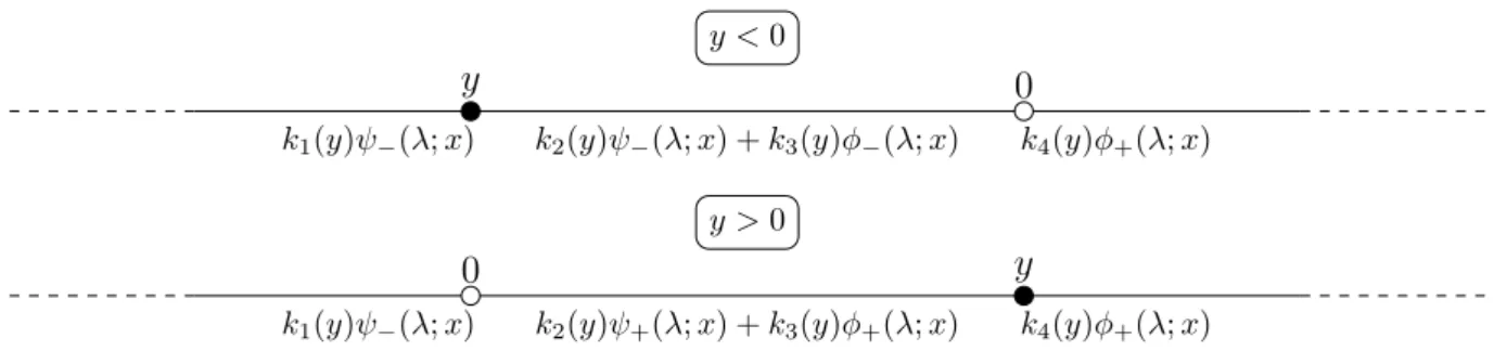
Proof. As the dimension is one, solving a second-order differential equation is equivalent to solve a first-order system. For 𝑥 ≥ 0, we have already found two independent solutions 𝜑+(𝜆; ·)
0 𝑦 𝑘1(𝑦)𝜓−(𝜆; 𝑥) 𝑘2(𝑦)𝜓−(𝜆; 𝑥) + 𝑘3(𝑦)𝜑−(𝜆; 𝑥) 𝑘4(𝑦)𝜑+(𝜆; 𝑥) 𝑦 < 0 0 𝑦 𝑘1(𝑦)𝜓−(𝜆; 𝑥) 𝑘2(𝑦)𝜓+(𝜆; 𝑥) + 𝑘3(𝑦)𝜑+(𝜆; 𝑥) 𝑘4(𝑦)𝜑+(𝜆; 𝑥) 𝑦 > 0
Figure 1: Splitting the state space to define superpositions.
Any solution to 𝒜𝐵𝑥,(𝑎
+,𝜌+,𝑏+)𝑓 (𝑥) = 𝜆𝑓 (𝑥) on 𝐽 ⊂ [0, +∞[ is thus locally a superposition of
𝜑+(𝜆; ·) and 𝜓+(𝜆; ·). A similar superposition can be considered for 𝑥 < 0 with two independent
solutions 𝜑−(𝜆; ·) and 𝜓−(𝜆; ·).
We have the following picture: To take (3.2)-(3.3) into account, the space is split into the intervals ]−∞, 0 ∧ 𝑦], ]0 ∧ 𝑦, 0 ∨ 𝑦[ and [0 ∨ 𝑦, +∞[ (See Figure 1).
Case 𝑦 ≥ 0. Let us set:
𝑘+1(𝑦) = 𝑐+1𝜑+(𝜆; 𝑦), 𝑘2+(𝑦) = 𝑐 + 2𝜑+(𝜆; 𝑦), 𝑘+3(𝑦) = 𝑐+3𝜑+(𝜆; 𝑦) and 𝑘4+(𝑦) = 𝑐 + 2𝜑+(𝜆; 𝑦) + 𝑐+3𝜓+(𝜆; 𝑦).
We look for the resolvent kernel under the form (3.11). Our choice ensures from that as 𝑥 → ∞, 𝑔(𝜆; 𝑥, 𝑦) decreases to 0. If there are other boundary conditions, then the functions 𝜑−and 𝜓+
may be introduced as well on the set {𝑥 ≤ 0} or {𝑥 ≥ 𝑦}.
The interface conditions at 0 and 𝑦 are linear ones. Conditions (3.5), (3.3) and (3.6) lead us to solve 𝑁𝑦≥0(𝜆, 𝑦)k+(𝑦) = f with f = ⎡ ⎢ ⎢ ⎣ 0 0 0 2 ⎤ ⎥ ⎥ ⎦ , k+(𝑦) = ⎡ ⎢ ⎢ ⎣ 𝑘1+(𝑦) 𝑘2+(𝑦) 𝑘3+(𝑦) 𝑘4+(𝑦) ⎤ ⎥ ⎥ ⎦ and 𝑁𝑦≥0(𝜆, 𝑦) = ⎡ ⎢ ⎢ ⎣ 𝜓−(𝜆; 0) −𝜑+(𝜆; 0) −𝜓+(𝜆; 0) 0 D𝑆− 𝑥 𝜓−(𝜆; 0) −D𝑆𝑥+𝜑+(𝜆; 0) D𝑆𝑥+𝜓+(𝜆; 0) 0 0 𝜑+(𝜆; 𝑦) 𝜓+(𝜆; 𝑦) −𝜑+(𝜆; 𝑦) 0 D𝑆+ 𝑥 𝜑+(𝜆; 𝑦) D𝑆𝑥+𝜓+(𝜆; 𝑦) −D𝑆𝑥+𝜑+(𝜆; 𝑦) ⎤ ⎥ ⎥ ⎦ .
Case 𝑦 < 0. Let us set:
𝑘1−(𝑦) = 𝑐−3𝜑−(𝜆; 𝑦) + 𝑐−2𝜓−(𝜆; 𝑦), 𝑘2−(𝑦) = 𝑐 −
3𝜓−(𝜆; 𝑦),
𝑘3−(𝑦) = 𝑐−2𝜓−(𝜆; 𝑦), 𝑘4−(𝑦) = 𝑐−1𝜓−(𝜆; 𝑦).
We look for the resolvent kernel under the form (3.12). Conditions (3.5), (3.3) and (3.6) lead us to solve 𝑁𝑦<0(𝜆, 𝑦)k−(𝑦) = f with f = ⎡ ⎢ ⎢ ⎣ 0 0 0 2 ⎤ ⎥ ⎥ ⎦ , k−(𝑦) = ⎡ ⎢ ⎢ ⎣ 𝑘1−(𝑦) 𝑘2−(𝑦) 𝑘3−(𝑦) 𝑘4−(𝑦) ⎤ ⎥ ⎥ ⎦
and 𝑁𝑦<0(𝜆, 𝑦) = ⎡ ⎢ ⎢ ⎣ 0 𝜑−(𝜆; 0) 𝜓−(𝜆; 0) −𝜑+(𝜆; 0) 0 D𝑆− 𝑥 𝜑−(𝜆; 0) D𝑆𝑥−𝜓−(𝜆; 0) −D𝑆𝑥+𝜑+(𝜆; 0) 𝜓−(𝜆; 𝑦) −𝜑−(𝜆; 𝑦) −𝜓−(𝜆; 𝑦) 0 D𝑆− 𝑥 𝜓−(𝜆; 𝑦) −D𝑆𝑥−𝜑−(𝜆; 𝑦) −D𝑆𝑥−𝜓−(𝜆; 𝑦) 0 ⎤ ⎥ ⎥ ⎦ .
The general formula follows from algebraic manipulations.
Remark3.4. The distribution of many random variables (hitting time, occupation time) related to a diffusion may be recovered from the minimal pairs (𝜑, 𝜓) (see e.g. [50]). One finds also the minimal pair (𝜑, 𝜓) of 𝒜𝐵
𝑥,(𝑎,𝜌,𝑏) through (3.7). Since 𝜑(𝜆; 0) = 𝜓(𝜆; 0) = 𝜑±(0) = 𝜓±(0) = 1,
the Wronskian 𝑊 between 𝜑 and 𝜓 is given by
𝑔(𝜆; 0, 0) = 2 𝑊 = 𝑐 + 1 = 𝑐 − 1 = 2 WrSPN[𝜑+, 𝜓−](𝜆; 0) so that 𝑊 = WrSPN[𝜑+, 𝜓−](𝜆; 0).
It is immediate that 𝑔(𝜆; 0, 𝑦)/𝑔(𝜆; 0, 0) = 𝜑(𝜆; 𝑦)1𝑦≥0+ 𝜓(𝜆; 𝑦)1𝑦<0and thereby
𝜓(𝜆; 𝑦) = 𝜓−(𝑦) if 𝑦 ≤ 0 and 𝜑(𝜆; 𝑦) = 𝜑+(𝑦) if 𝑦 ≥ 0. Moreover, 𝜓(𝜆; 𝑦) = 𝑊 2 𝑔(𝜆; 𝑥, 𝑦) 𝜑(𝜆; 𝑥) = 𝑊 2 𝑔(𝜆; 𝑥, 𝑦) 𝜑+(𝑥) for 0 ≤ 𝑦 < 𝑥
Thus, 𝜓(𝜆; 𝑦) is recovered from the last coefficient in (3.11) and the condition 𝜓(𝜆; 0) = 1, so that 𝜓(𝜆; 𝑦) = 𝑐 + 2𝜑+(𝜆; 𝑦) + 𝜓+(𝜆; 𝑦)𝑐+3 𝑐+1 for 𝑦 ≥ 0. Similarly, 𝜑(𝜆; 𝑦) = 𝑐 − 3𝜑−(𝜆; 𝑦) + 𝑐 − 2𝜓−(𝜆; 𝑦) 𝑐−1 for 𝑦 < 0. It can be easily verified by a direct computation that 𝑐±3 + 𝑐±2 = 𝑐±1.
4
Particular case of piecewise constant coefficients
In this section, we give a closed form expression of the resolvent kernel 𝑟(𝜆; 𝑥, 𝑦) as well as a closed form expression of the transition function 𝑞(𝑡, 𝑥, 𝑦) when the coefficients are piecewise constants.
4.1
Reduction to the drifted Skew Brownian motion
We actually reduce the number of involved variables problem by performing a simple change of variable. Although everything here can be done in the context of Partial Differential Equations, we illustrate this change of variable by their relations on stochastic processes.
Proposition 4.1 ( [19, 30, 48]). When (𝑎, 𝜌, 𝑏) ∈ M, the operator (𝒜𝐵𝑥,(𝑎,𝜌,𝑏), Dom(𝒜𝐵𝑥,(𝑎,𝜌,𝑏))) is the infinitesimal generator of a Feller process𝑋.
Feller processes associated to knotted operators with coefficients in H◁▷can be expressed in term of solutions to Stochastic Differential Equations with Local Time, an aspect which we do not develop here (See e.g. [14, 15, 38, 39] among many other references).
We now restrict ourselves to piecewise constant coefficients. Notation4.1. We define
K:= {𝑓 : R → R | 𝑓 is constant}
and P := {(𝑎, 𝜌, 𝑏) | 𝑎, 𝜌 ∈ K ∩ C and 𝑏 ∈ K ∩ B} ⊂ H. We then identify constants and functions in K.
We recall Notation 3.1.
Definition 4.1 (Drifted Skew Brownian motion). For some constants 𝛽 ∈ (0, 1) and 𝛾−, 𝛾+∈ R,
we define
(𝑎−, 𝜌−, 𝑏−) := (︀1 − 𝛽, (1 − 𝛽)−1, 𝛾−)︀ ∈ P,
(𝑎+, 𝜌+, 𝑏+) := (︀𝛽, 𝛽−1, 𝛾+)︀ ∈ P
as well as
DSBM(𝛽, 𝛾+, 𝛾−) := (𝑎−, 𝜌−, 𝑏−) ◁▷ (𝑎+, 𝜌+, 𝑏+) ∈ P◁▷.
The process𝑌 associated to (𝒜𝐵
𝑥,DSBM(𝛽,𝛾+,𝛾−), Dom(𝒜
𝐵
𝑥,DSBM(𝛽,𝛾+,𝛾−))) is called a drifted Skew
Brownian motion (DSBM). It is a Skew Brownian motion if 𝛾− = 𝛾+ = 0 [39]. It is a Brownian
motion with piecewise constant drift when𝛽 = 1/2 and a Brownian motion when in addition 𝛾− = 𝛾+= 0.
The next result follows from straightforward computations.
Lemma 4.1. Let 𝑋 be the stochastic process associated to the operator 𝒜𝐵
𝑥,(𝑎,𝜌,𝑏) with piecewise
constant coefficients(𝑎, 𝜌, 𝑏) ∈ P◁▷. For𝜅−, 𝜅+ > 0 we set 𝐺(𝑥) := 𝜅(𝑥) · 𝑥 be a piecewise
linear change of variable with 𝜅 := 𝜅− ◁▷ 𝜅+ ∈ K◁▷. Then𝑌 = 𝐺(𝑋) is associated to the
operator𝒜𝐵
𝑥,(𝑎𝜅,𝜌𝜅,𝑏𝜅)with(𝑎𝜅, 𝜌𝜅, 𝑏𝜅) ∈ P◁▷.
Proposition 4.2 (Reduction to a drifted Skew Brownian motion). Let 𝑋 be the stochastic process associated to the operator𝒜𝐵
𝑥,(𝑎,𝜌,𝑏)with piecewise constant coefficients(𝑎, 𝜌, 𝑏) ∈ P ◁▷.
Consider the piecewise linear change of variable𝐺(𝑥) = √ 1
𝑎(𝑥)𝜌(𝑥)𝑥. The process 𝑌 = 𝐺(𝑋) is a DSBM with coefficients (𝑎𝑌, 𝜌𝑌, 𝛾) = (︂ 𝑎 √ 𝑎𝜌, 𝜌 √ 𝑎𝜌, 𝑏 √ 𝑎𝜌 )︂ = DSBM (𝛽, 𝛾+, 𝛾−) with 𝛽 = √ 𝑎+/ √ 𝜌+ √ 𝑎+/ √ 𝜌++ √ 𝑎−/ √ 𝜌− , 𝛾+ = 𝑏+ √ 𝑎+𝜌+ and𝛾− = 𝑏− √ 𝑎−𝜌− .
The resolvent kernel r𝒜𝐵
𝑥,(𝑎,𝜌,𝑏) of𝑋 associated to (𝑎, 𝜌, 𝑏) ∈ H is given by
r𝒜𝐵
𝑥,(𝑎,𝜌,𝑏)(𝜆; 𝑥, 𝑦) =
rDSBM(𝛽,𝛾+,𝛾−)(𝜆; 𝐺(𝑥), 𝐺(𝑦))
√︀𝑎(𝑦)𝜌(𝑦) (4.1) where rDSBM(𝛽,𝛾+,𝛾−)is the resolvent kernel of the DSBM. A similar relation holds for the density.
Proof. The identification of (𝑎𝑌, 𝜌𝑌, 𝛾) follows from Lemma 4.1. The process 𝑌 is characterized
by its scale function and its speed measure. Multiplying the scale function by a constant 𝑐 > 0 and dividing the speed measure by the same constant 𝑐 < 0 give rise to the same process. Choosing 𝑐 = (√𝑎+/ √ 𝜌++ √ 𝑎−/ √
𝜌−)−1leads to identify the process 𝑌 as the one associated
to DSBM (𝛽, 𝛾+, 𝛾−).
The advantage of using 𝐺 is that the number of parameters defining (𝑎, 𝜌, 𝑏) ∈ P◁▷, which is 6, is reduced to only 3: (𝛽, 𝛾+, 𝛾−). Besides, the parameter 𝛽 has an explicit interpretation in term
of stochastic process as the parameter of a Skew Brownian motion [39, 42]. We use the special form of the drifted Skew Brownian motion to get explicit expressions for the densities and the resolvent kernel of 𝑋 from the ones of 𝑌 = 𝐺(𝑋).
4.2
Explicit computations of the resolvent kernel of the DSBM
The coefficients of the DSBM are piecewise constant ones. The results of Section 3 can therefore be used. According to Proposition 4.2, it is enough to compute rDSBM(𝛽,𝛾+,𝛾−)to get an expression
for the resolvent kernel r𝒜𝐵
𝑥,(𝑎,𝜌,𝑏) with (𝑎, 𝜌, 𝑏) ∈ P
◁▷.
The speed measure 𝑚 of the process 𝑌 associated to 𝒜𝐵𝑥,DSBM(𝛽,𝛾
+,𝛾−) is
𝑚(𝑥) = {︃
𝑚+(𝑥) := 𝛽𝑒2𝛾+𝑥 if 𝑥 ≥ 0,
𝑚−(𝑥) := (1 − 𝛽)𝑒2𝛾−𝑦 if 𝑥 < 0.
and its scale function 𝑆 is 𝑆(𝑥) =∫︀0𝑥𝑠(𝑦) d𝑦 with 𝑠(𝑥) = 1/𝑚(𝑥). According to Proposition 5.3, rDSBM(𝛽,𝛾+,𝛾−)(𝜆, 𝑥, 𝑦) = 𝑔(𝜆, 𝑥, 𝑦)𝑚(𝑦), (4.2)
where 𝑔(𝜆, 𝑥, 𝑦) is given by Theorem 3.1 in which the minimal pairs (𝜑±(𝜆; ·), 𝜓±(𝜆; ·)) are
𝜓±(𝜆; 𝑥) = exp (︂(︂ −𝛾±+ √︁ 𝛾2 ±+ 2𝜆 )︂ 𝑥 )︂ for 𝑥 ∈ R and 𝜑±(𝜆; 𝑥) = exp (︂(︂ −𝛾±− √︁ 𝛾2 ±+ 2𝜆 )︂ 𝑥 )︂ for 𝑥 ∈ R.
It is here noteworthy that these minimal pairs do not depend on 𝛽.
The next proposition is an application of Theorem 3.1 and (4.2) after some algebraic manipulation. Its formulation requires the following bunch of notations
Notation4.2. We set
𝜆+ := 𝛾+2 + 2𝜆 > 0, 𝜆−:= 𝛾−2 + 2𝜆 > 0 and 𝜇 := 𝛽𝛾+− (1 − 𝛽)𝛾−.
and define the constants
Θ := 𝜇 + 𝛽√︀𝜆++ (1 − 𝛽) √︀ 𝜆−, Θ+:= −𝜇 + 𝛽 √︀ 𝜆+− (1 − 𝛽) √︀ 𝜆−and Θ− := −𝜇 − 𝛽 √︀ 𝜆++ (1 − 𝛽) √︀ 𝜆−.
Proposition 4.3. With the above notations on Θ, Θ+,Θ−,𝜆+ and𝜆−, for any𝜆 > 0, 𝑥, 𝑦 ∈ R, rDSBM(𝛽,𝛾+,𝛾−)(𝜆; 𝑥, 𝑦) = 1 Θ× ⎧ ⎪ ⎪ ⎪ ⎪ ⎪ ⎪ ⎪ ⎪ ⎪ ⎪ ⎪ ⎪ ⎪ ⎪ ⎪ ⎪ ⎪ ⎪ ⎪ ⎪ ⎪ ⎪ ⎪ ⎪ ⎪ ⎨ ⎪ ⎪ ⎪ ⎪ ⎪ ⎪ ⎪ ⎪ ⎪ ⎪ ⎪ ⎪ ⎪ ⎪ ⎪ ⎪ ⎪ ⎪ ⎪ ⎪ ⎪ ⎪ ⎪ ⎪ ⎪ ⎩ 2𝛽 exp(𝛾+𝑦 −√︀𝜆+𝑦 − 𝛾−𝑥 +√︀𝜆−𝑥) if𝑥 ≤ 0 ≤ 𝑦, 𝜆−1/2+ exp(𝛾+(𝑦 − 𝑥)) × [︁ Θ exp(−√︀𝜆+(𝑦 − 𝑥)) + Θ+exp(−√︀𝜆+(𝑥 + 𝑦)) ]︁ if0 < 𝑥 ≤ 𝑦, 𝜆−1/2+ exp(−𝛾+(𝑥 − 𝑦)) × [︁ Θ exp(−√︀𝜆+(𝑥 − 𝑦)) + Θ+exp(−√︀𝜆+(𝑥 + 𝑦)) ]︁ if0 < 𝑦 ≤ 𝑥, 2(1 − 𝛽) exp(𝛾−𝑦 − 𝛾+𝑥 +√︀𝜆−𝑦 −√︀𝜆+𝑥) if𝑦 < 0 ≤ 𝑥, 𝜆−1/2− exp(−𝛾−(𝑥 − 𝑦)) × [︁ Θ exp(−√︀𝜆−(𝑥 − 𝑦)) + Θ−exp(√︀𝜆−(𝑦 + 𝑥)) ]︁ if𝑦 ≤ 𝑥 < 0, 𝜆−1/2− exp(𝛾−(𝑦 − 𝑥)) × [︁ Θ exp(−√︀𝜆−(𝑦 − 𝑥)) + Θ−exp(√︀𝜆−(𝑦 + 𝑥)) ]︁ if𝑥 ≤ 𝑦 < 0. (4.3)
4.3
Some explicit expressions for the transition density function
The transition density function may be recovered from the Laplace inversion of the resolvent kernel [48]. Here we propose various explicit expressions of the transition density function qDSBM(𝛽,𝛾+,𝛾−)whenever we manage to derive the Laplace inversions of rDSBM(𝛽,𝛾+,𝛾−).
Notation4.3. We define sgn(𝑦) := 1𝑦≥0− 1𝑦<0, erf(𝑥) := √2 𝜋 ∫︁ 𝑥 0
𝑒−𝑣2d𝑣 and erfc(𝑥) := 1 − erf(𝑥) = √2 𝜋
∫︁ +∞
𝑥
𝑒−𝑣2d𝑣.
4.3.1 General considerations on Laplace inversion
The density results from a Laplace inversion of the resolvent kernel, when possible. The general case seems to be difficult to deal with as it involves a denominator of type 𝑎+√𝑐 + 2𝜆+√𝑑 + 2𝜆 for some constants 𝑎, 𝑐, 𝑑. We did not found any expression for this in the literature. Yet we can see from the expression of Θ+, Θ−and Θ that some cases lead to simplifications.
4.3.2 The situations in which 𝜆+= 𝜆−
We first consider the situation in which 𝜆+ = 𝜆−. It may happen when 𝛽+ = 𝛽− = 0 (Skew
Brownian motion), 𝛾+ = 𝛾−̸= 0 (Skew Brownian motion with a constant drift), or 𝛾+= −𝛾−
(Skew Brownian motion with a bang-bang drift). In this case, Θ = 𝜇 +√︀𝜆+, Θ+= −𝜇 + (2𝛽 − 1) √︀ 𝜆+and Θ− = −𝜇 + √︀ 𝜆+.
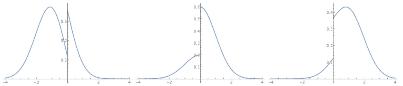
Figure 2: The density qDSBM(𝛽,0,0)(𝑡, 𝑥, 𝑦) of the SBM for 𝛽 = 34 at time 𝑡 = 1 for the initial
positions: 𝑥 = −1, 𝑥 = 0 and 𝑥 = 1 (from left to right).
Let us recall some classical formula on inverse Laplace. Lemma 4.2 (See [1]). For 𝑘 ≥ 0, 𝑐 > 0, 𝜇 ∈ R,
ℒ−1 (︂ 1 √ 𝜆𝑒 −𝑘√𝜆 )︂ = √1 𝜋𝑡𝑒 −𝑘2 4𝑡, (4.4) ℒ−1(𝑓 (𝑐𝜆 + 𝑑)) = 1 𝑐𝑒 −𝑑 𝑐𝑡ℒ−1(𝑓 )(︂ 𝑡 𝑐 )︂ , (4.5) ℒ−1 (︃ 𝑒−𝑘 √ 𝜆 𝜇 +√𝜆 )︃ = √1 𝜋𝑡𝑒 −𝑘2 4𝑡 − 𝜇𝑒𝜇𝑘𝑒𝜇 2𝑡 erfc (︂ 𝜇√𝑡 + 𝑘 2√𝑡 )︂ . (4.6) In addition, when 𝜇 ̸= 0, 𝜇 √︀𝜆+(𝜇 +√︀𝜆+) = 1 √︀𝜆+ + −1 𝜇 +√︀𝜆+ so that 1 √︀𝜆+ Θ+ Θ = 2𝛽 𝜇 +√︀𝜆+ − 1 √︀𝜆+ and 1 √︀𝜆+ Θ− Θ = 2 𝜇 +√︀𝜆+ − 1 √︀𝜆+ .
The formula of Lemma 4.2 are sufficient to compute termwise the inverse Laplace transforms of the resolvent kernel when 𝜆+ = 𝜆−.
4.3.3 The Skew Brownian Motion
The SBM of parameter 𝛽 ∈ (0, 1) is given by the choice of the coefficients DSBM(𝛽, 0, 0). Hence, 𝜆+ = 𝜆−and 𝜇 = 0. Thus, after an application of (4.4)-(4.5) to (5.13) as well as some
rewriting, qDSBM(𝛽,0,0)(𝑡, 𝑥, 𝑦) = 1 √ 2𝜋𝑡𝑒 −(𝑦−𝑥)22𝑡 + sgn(𝑦)(2𝛽 − 1)√1 2𝜋𝑡𝑒 −(|𝑦|+|𝑥|)22𝑡 .
This density was obtained in [58] through a probabilistic argument. Some plots are given in Figure 2.
4.3.4 The Skew Brownian Motion with a constant drift
The density of the SBM with a constant drift, which corresponds to the coefficient DSBM(𝛽, 𝛾, 𝛾) for some 𝛾 ̸= 0 was computed in [2, 3, 17, 24] with different probabilistic arguments.
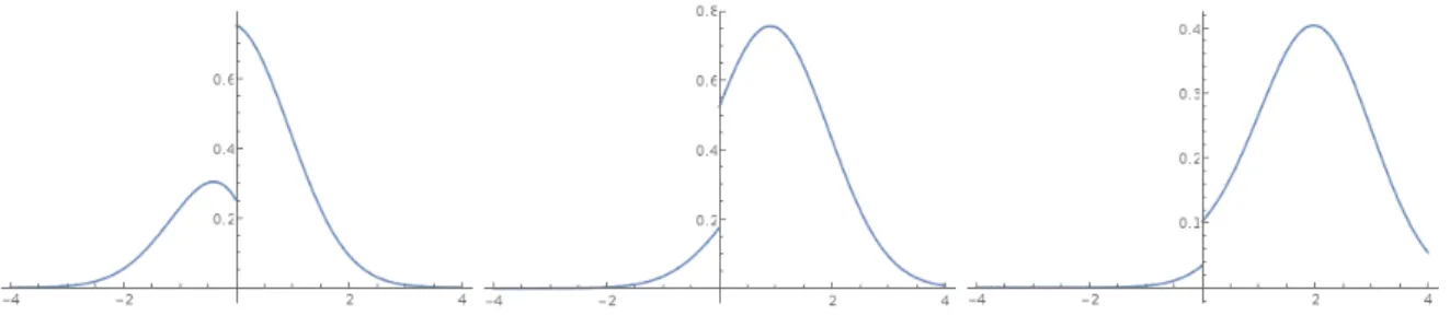
Figure 3: The density qDSBM(𝛽,𝛾,𝛾)(𝑡, 𝑥, 𝑦) of the SBM for 𝛽 = 34 with a constant drift 𝛾 = 2 at
time 𝑡 = 1 for the initial positions: 𝑥 = −1, 𝑥 = 0 and 𝑥 = 1 (from left to right).
Figure 4: The density qDSBM(𝛽,𝛾,−𝛾)(𝑡, 𝑥, 𝑦) of the SBM for 𝛽 = 34 with a Bang bang drift 𝛾 = 2
at time 𝑡 = 1 for the initial positions 𝑥 = −1, 𝑥 = 0 and 𝑥 = 1 (from left to right).
In this case, 𝜆+ = 𝜆− =√︀𝛾2+ 2𝜆 and 𝜇 = (2𝛽 − 1)𝛾. With the formula of Lemma 4.2 (see
Figure 3), qDSBM(𝛽,𝛾,𝛾)(𝑡, 𝑥, 𝑦) = 1 √ 2𝜋𝑡𝑒 −𝛾𝑡−(𝑦−𝑥))2 2𝑡 + sgn(𝑦)(2𝛽 − 1)√1 2𝜋𝑡𝑒 −(|𝑦|+|𝑥|)2 2𝑡 𝑒−𝛾 2 𝑡 2𝑒𝛾(𝑦−𝑥) + sgn(𝑦)(1𝑦<0− 𝛽)𝛾(2𝛽 − 1)𝑒𝛾(2𝛽−1)(|𝑦|+|𝑥|)𝑒𝛾(𝑦−𝑥)𝑒2𝛾 2𝛽(𝛽−1)𝑡 × erfc (︃ 𝛾(2𝛽 − 1) √︂ 𝑡 2 + |𝑦| + |𝑥| √ 2𝑡 )︃ .
We recover the density obtained in [2,17] up to a conversion of erfc to its probabilistic counterpart.
4.3.5 The Bang-Bang Skew Brownian Motion
The Bang-Bang SBM is the diffusion corresponding to the choice of the coefficients DSBM(𝛽, 𝛾, −𝛾) for some 𝛾 ̸= 0. This process was introduced in [23]. It may also be called a Skew Brownian motion with dry friction[6].
In this case, 𝜆+ = 𝜆−=√︀𝛾2+ 2𝜆 and 𝜇 = 𝛾. Again with Lemma 4.2 (see Figure 4)
qDSBM(𝛽,𝛾,−𝛾)(𝑡, 𝑥, 𝑦) = 1 √ 2𝜋𝑡𝑒 −(𝛾𝑡−sgn(𝑦)(𝑦−𝑥))22𝑡 +sgn(𝑦)(2𝛽−1)√1 2𝜋𝑡𝑒 −(|𝑦|+|𝑥|)22𝑡 𝑒−𝛾2 𝑡2𝑒𝛾(|𝑦|−|𝑥|) + sgn(𝑦)(1𝑦<0− 𝛽)𝛾𝑒2𝛾|𝑦| erfc (︃ 𝛾 √︂ 𝑡 2 + |𝑦| + |𝑥| √ 2𝑡 )︃ .
This is the expression given in [23] up to a conversion of erfc into its probabilistic counterpart. It is also the one given in [6].
4.3.6 The constant Péclet case (𝜇 = 0)
We consider that 𝛾− ̸= 𝛾+and 𝛽 ̸= 0. Another situation in which a simplification occurs is when
𝜇 = 𝛽𝛾+− (1 − 𝛽)𝛾− = 0, which means that
𝛾−= 𝜅𝛾+with 𝜅 =
𝛽
1 − 𝛽 or equivalently 𝜇 = 0 when 𝛽 ̸= 1
2. (4.7) Remark4.1. This assumption on 𝛾+and 𝛾−is natural. Then 𝑌 is obtained through the
transfor-mation of Proposition 4.2 from a process 𝑋 with piecewise constant coefficients (𝑎, 𝜌, 𝑏), then (4.7) is satisfied when 𝑏+ 𝜌+ = 𝑏− 𝜌− .
When 𝑎 = 1, the ratio 𝑏/𝜌 is called the Péclet number. It is a dimensionless quantity which plays a very important role in fluid mechanics by characterizing the effect of the convection against the diffusion and vice versa.
We give the density starting from 0. Actually, for 𝑥 < 0 < 𝑦, the strong Markov property implies that
qDSBM(𝛽,𝛾+,𝛾−)(𝑡, 𝑥, 𝑦) =
∫︁ 𝑡
0
qDSBM(𝛽,𝛾+,𝛾−)(𝑡 − 𝑠, 0, 𝑦)𝑞−(𝑥, 𝑠) d𝑠
where 𝑞−(𝑥, 𝑠) is the density of the hitting time of 0 for the Brownian motion with drift 𝛾−.
The Laplace transform of 𝑞−(𝑥, 𝑠) is nothing more than 𝜓1(𝑥). A similar computation holds for
𝑦 < 0 < 𝑥.
Proposition 4.4. For any 𝑡 ≥ 0 and DSBM(𝛽, 𝛾, 𝜅𝛾), with 𝛾(𝑦) = ((𝜅𝛾) ◁▷ 𝛾)(𝑦),
qDSBM(𝛽,𝛾,𝜅𝛾)(𝑡, 0, 𝑦) = 2 (1𝑦<0− 𝛽)2 (2𝛽 − 1)√2𝜋𝑡𝑒 −(𝛾(𝑦)2𝑡−𝑦)22𝑡 + 𝛾(𝑦) (1𝑦<0− 𝛽) 2 2(2𝛽 − 1) (︃ erfc (︃ 𝑦 √ 2𝑡− 𝛾(𝑦) √︂ 𝑡 2 )︃ − 𝑒2𝛾(𝑦) 𝑦erfc (︃ 𝑦 √ 2𝑡 + 𝛾(𝑦) √︂ 𝑡 2 )︃)︃ − 𝛽 (1 − 𝛽) 𝑒 𝛾(𝑦) 𝑦 2(2𝛽 − 1)𝜋 ∫︁ 𝑡 0 𝑒−𝛾(𝑦)2 𝜏2 ∫︁ 𝛾2(−𝑥)−𝛾2(𝑥) 0 sin(𝑦√𝑟)√︀𝛾2(−𝑥) − 𝛾2(𝑥) − 𝑟𝑒−𝑟 𝜏2 d𝑟 d𝜏 +𝛽 (1 − 𝛽) 𝑒 𝛾(𝑦) 𝑦 2(2𝛽 − 1)𝜋 ∫︁ 𝑡 0 𝑒−(𝛾(−𝑦)2) 𝜏2 ∫︁ +∞ 0 cos(𝑦√︀𝑟 + 𝛾2(−𝑥) − 𝛾2(𝑥))√𝑟𝑒−𝑟 𝜏2 d𝑟 d𝜏.
Proof. When (4.7) holds, 1 Θ = 𝛽√︀𝜆+− (1 − 𝛽)√︀𝜆− 𝛽2𝜆 +− (1 − 𝛽)2𝜆− = 𝛽√︀𝜆+− (1 − 𝛽)√︀𝜆− 2𝜆(2𝛽 − 1) . (4.8) In addition, Θ+= (2𝛽 − 1)Θ and Θ− = Θ.
Each line in the right-hand side of (4.3) is easily inverted using (4.4) excepted when 𝑦 < 0 ≤ 𝑥 and 𝑥 ≤ 0 < 𝑦.
To simplify the formula, we consider starting at 𝑥 = 0. With (4.8), rDSBM(𝛽,𝜅𝛾+,𝛾+)(𝜆, 0, 𝑦) = 𝛽√︀𝜆+− (1 − 𝛽)√︀𝜆− (2𝛽 − 1)𝜆 (︁ 𝛽𝑒(𝛾+− √ 𝜆+)𝑦1 𝑦≥0+ (1 − 𝛽)𝑒(𝛾−+ √ 𝜆−)𝑦 1𝑦<0 )︁ .
We focus on the term for 𝑦 > 0, the other term being treated by symmetry. With (4.5), we could use 𝜆+instead of 𝜆 as the parameter for the Laplace transform. Since 2𝜆 = 𝜆+− 𝛾+2,
√︀𝜆+ 𝜆+− 𝛾+2 𝑒− √ 𝜆+𝑦 = 𝛾+ (𝜆+− 𝛾+2)√︀𝜆+ 𝑒− √ 𝜆+𝑦 + 1 √︀𝜆+ 𝑒− √ 𝜆+𝑦.
Hence, the inverse Laplace of the first term in the right-hand side of the above expression can be computed with Lemma B.1, given in Appendix B, while the second term is inverted using (4.4). Let us write 𝜈 = 𝛾2 −− 𝛾+2 = 𝛾+2(2𝛽 − 1)/(1 − 𝛽)2. Thus, 𝜆− = 𝜆++ 𝜈. Hence, √︀𝜆− 𝜆 𝑒 −√𝜆+𝑦 = 2√︀𝜆++ 𝜈 𝜆+− 𝛾+2 𝑒− √ 𝜆+𝑦.
Using the convolutional property of the Laplace transform and since ℒ−1(1/(𝑎 + 𝜆))(𝑡) = exp(𝑎𝑡), we get that
ℒ−1 (︃ 2√︀𝜆++ 𝜈 𝜆+− 𝛾+2 𝑒− √ 𝜆+𝑦 )︃ = 1 2 ∫︁ 𝑡 0 𝑒− 𝛾2+ 2 𝜏ℒ−1(︁√︀𝜆++ 𝜈𝑒− √ 𝜆+𝑦 )︁ (𝜏 ) d𝜏.
We conclude using Lemma B.2, given in Appendix B.
The case 𝑦 < 0 is treated similarly. The final formula is obtained by gathering all the terms.
Such closed form formula open the door to numerical simulation using a class of Monte Carlo methods called particles tracking techniques [53, 62] as shown in the two following Sections.
5
Particle tracking techniques to solve advection-diffusion
prob-lems with one discontinuity
In this section, we show that the methodology derived in the Sections 3 and 4 is useful for solving advection-diffusion problems with particle tracking techniques. We consider here an infinite one dimensional porous medium with one discontinuity. Subsection 5.1 recall the forward formulation of advection-diffusion problems with one discontinuity. Subsection 5.2 emphasizes that the dynamic of the particles in particle tracking techniques is governed by the backward formulation. Then it shows that the probability transition function of the particles can be obtained by the Laplace inversion of the resolvent kernel r𝒜𝐵
𝑥,(𝑎,1,𝑏)given in Proposition 4.2 (with 𝜌 = 1
5.1
Problem settings: the forward formulation
Without loss of generality, let us consider a single interface at the point 𝑦 = 0 between two layers possessing different diffusion/advective coefficients.
Let us consider a solute evolving in an infinite one dimensional porous medium described by a diffusivity 𝑎 = 𝑎−◁▷ 𝑎+ ∈ C◁▷and an advective force 𝑏 = 𝑏− ◁▷ 𝑏+∈ B◁▷.
The concentration u(𝑡, ·) at time 𝑡 is given by the solution of the advection-diffusion equation: 𝜕𝑡u(𝑡, 𝑦) − ℒ𝐹𝑦u(𝑡, 𝑦) = 0, 𝑡 > 0, 𝑦 ̸= 0, (5.1)
u(𝑡, ·)−−−→weakly
𝑡→0 𝜈, (5.2)
𝑎−(0−)𝜕𝑦u(𝑡, 0−) − 𝑏−(0−)u(𝑡, 0−) = 𝑎+(0+)𝜕𝑦u(𝑡, 0+) − 𝑏+(0+)u(𝑡, 0+), (5.3)
u(𝑡, 0−) = u(𝑡, 0+), (5.4) where ℒ𝐹𝑦u(𝑡, 𝑦) = ⎧ ⎪ ⎨ ⎪ ⎩ ℒ𝐹 −,𝑦u(𝑡, 𝑦) = 1 2𝜕𝑦(𝑎−(𝑦)𝜕𝑦u(𝑡, 𝑦)) − 𝜕𝑦(𝑏−(𝑦)u(𝑡, 𝑦)) if 𝑦 < 0, ℒ𝐹 +,𝑦u(𝑡, 𝑦) = 1 2𝜕𝑦(𝑎+(𝑦)𝜕𝑦u(𝑡, 𝑦)) − 𝜕𝑦(𝑏+(𝑦)u(𝑡, 𝑦)) if 𝑦 > 0. (5.5)
Remark5.1. When div(𝑏±(𝑦)) = 0 at a point 𝑦 ̸= 0 (the fluid is incompressible around 𝑦), then
𝜕𝑦(𝑏±(𝑦)u(𝑡, 𝑦)) = 𝑏±(𝑦)𝜕𝑦u(𝑡, 𝑦).
Remark5.2. The conditions (5.3)-(5.4) ensure the mass conservation and the continuity of the density u(𝑡, 𝑦) at the interface. They have a natural interpretation in term of modeling [32]. The differential operator ℒ𝐹
𝑦 appears as the knotting of ℒ𝐹−,𝑦 and ℒ𝐹+,𝑦. Yet (5.5) is not sufficient
to define an effective functional operator as its domain, that is the space of functions on which it acts, is not specified. In particular, the behavior at 0 shall be given [37].
Let L2(R) be the space of square summable functions equipped with the usual norm ‖ · ‖2
and H1(R) be the Sobolev space of functions in L2(R) admitting a weak derivative in L2(R).
When the initial mass repartition 𝜈 has a density 𝑛 with respect to the Lebesgue measure which belongs to L2(R), the advection-diffusion equation (5.1)-(5.4) has to be understood in its variational form. Therefore, its solution u(𝑡, 𝑥) is sought in the intersection of L2([0, 𝑇 ]; H1(R))
and 𝒞([0, 𝑇 ]; L2(R)) and we are naturally lead to let ℒ𝐹
𝑦 act on L2(R). Its domain Dom(ℒ𝐹𝑦) is
thus defined as
Dom(ℒ𝐹𝑦) :={︀u ∈ H1(R)⃒⃒ℒ𝐹𝑦u ∈ L2(R)}︀. Remark 5.3. If u ∈ H1(R) and ℒ𝐹
𝑦u ∈ L2(R), then it is easily seen that 𝑦 ↦→ 𝑎(𝑦)𝜕𝑦u(𝑦) +
𝑏(𝑦)u(𝑦) belongs to H1(R). As there exists a continuous version (the one we implicitly use) of a function in H1(R), u(𝑦) and 𝑎(𝑦)𝜕𝑦u(𝑦) are really defined for 𝑦 = 0− (resp. 𝑦 = 0+)
by continuity. Hence, the definition of Dom(ℒ𝐹
𝑦) directly implies the transmission conditions
[u]0 = 0 and [𝑎𝜕𝑦u+ 𝑏u]0 = 0, where [𝑓 ]0 = 𝑓 (0+) − 𝑓 (0−) for a function 𝑓 . Meanwhile, for
a solution u to (5.1)-(5.2) with u(𝑡, ·) ∈ Dom(ℒ𝐹𝑥), for any 𝑡 > 0, this naturally leads to the conditions (5.3)-(5.4).
Remark5.4. The problem (5.1)-(5.4) can be understood as a transmission problem (or diffraction problem) which is an alternative to the weak formulation. Roughly speaking, the solution is classical away from 0 with some interface conditions at 0 [33–35].
The formulation (5.1)-(5.4) is the one used in physics. It gives the density of particles at the position 𝑦 starting from a source density 𝜈. When the initial distribution is a Dirac mass, this is a Fokker-Planckor a Kolmogorov forward equation.
5.2
Principle of particle tracking techniques
We propose to consider a particle tracking technique to solve (5.1)-(5.4). According to this technique, the concentration of the solute at time 𝑡 can be derived from the positions of a plume of particles which are initially distributed with a probability measure 𝜈. It has a natural interpretation: each particle carries some part of the mass of the solute. For that purpose, we display a stochastic process 𝑋 such that u(𝑡, ·) is the density of 𝑋(𝑡) when the particles are initially distributed according to the measure 𝜈. The existence of such a process, even in presence of discontinuous coefficients, follows from [55].
The solution u(𝑡, 𝑦) to (5.1)-(5.4) is given by
u(𝑡, 𝑦) = ∫︁
R
𝜈( d𝑥)q(𝑡, 𝑥, 𝑦), (5.6)
where kernel q is also called the fundamental solution. It is the probability transition function that governs the dynamic of the particles. Indeed, since the problem is time-homogeneous, 𝑦 ↦→ q(𝑡, 𝑥, 𝑦) is the density of 𝑋(𝑠 + 𝑡) given 𝑋(𝑠) = 𝑥, for any 𝑠, 𝑡 ≥ 0. Hence, knowing q(𝑡, 𝑥, 𝑦) allows one to set-up a particle tracking scheme.
5.3
Dynamic of the particles and the backward formulation
The stochastic process we have to exhibit is actually the one so that
lim 𝑡→0 E𝑥[𝑓 (𝑋(𝑡))] − 𝑓 (𝑥) 𝑡 = ℒ 𝐵 𝑥𝑓 (𝑥), ∀𝑓 ∈ Dom(ℒ 𝐵 𝑥),
where E𝑥is the expectation of 𝑋 given 𝑋(0) = 𝑥 and ℒ𝐵𝑥 is the backward operator, also called
the infinitesimal generator of 𝑋. So the dynamic is read from the backward operator defined below.
5.3.1 The backward formulation
For suitable functions v : R+× R → R, we introduce the operator
ℒ𝐵 𝑦v(𝑡, 𝑦) := ⎧ ⎪ ⎨ ⎪ ⎩ ℒ𝐵 −,𝑦v(𝑡, 𝑦) = 1 2𝜕𝑦(𝑎−(𝑦)𝜕𝑦v(𝑡, 𝑦)) + 𝑏−(𝑦)𝜕𝑦v(𝑡, 𝑦) if 𝑦 < 0, ℒ𝐵 +,𝑦v(𝑦) = 1 2𝜕𝑦(𝑎+(𝑦)𝜕𝑦v(𝑡, 𝑦)) + 𝑏+(𝑦)𝜕𝑦v(𝑡, 𝑦) if 𝑦 > 0. (5.7)
We could deal with the equation
𝜕𝑡v(𝑡, 𝑦) − ℒ𝐵𝑦v(𝑡, 𝑦) = 0, 𝑡 > 0, 𝑦 ̸= 0, (5.8) v(𝑡, 𝑦) −−→ 𝑡→0 𝑓 (𝑦) ∈ L 2(R), (5.9) 𝑎−(𝑡, 0−)𝜕𝑦v(𝑡, 0−) = 𝑎+(𝑡, 0+)𝜕𝑦v(𝑡, 0+), (5.10) v(𝑡, 0−) = v(𝑡, 0+). (5.11) As above, we define Dom(ℒ𝐵𝑦) := {v ∈ H1(R) | ℒ𝐵𝑦v ∈ L2(R)}.
Since ℒ𝐵𝑦v ∈ L2(R) for v ∈ Dom(ℒ𝐵
𝑦), 𝑎(𝑦)𝜕𝑦v(𝑦) ∈ H1(R). Using the same argument as in
Remark 5.3, Dom(ℒ𝐵𝑦) is well defined. Besides, for a variational solution v to (5.8)-(5.9) with v(𝑡, ·) ∈ Dom(ℒ𝐵
𝑦), the condition (5.10)-(5.11) are implicitly satisfied for the proper choice of
the version of 𝑎∇v(𝑡, ·) which is continuous over R (and so is v(𝑡, ·)). This is why no interface conditions appear in the definition of the domain of ℒ𝐵𝑦.
Here it is noteworthy to look at the reverse sign of the advective term as well as the difference in the interface conditions of the forward and backward formulations. In fact, no advective term is involved in the interface conditions for the backward formulation. See Annexe A for more details.
The solution v(𝑡, 𝑦) to (5.8)-(5.11) is given by
v(𝑡, 𝑥) = ∫︁
R
q(𝑡, 𝑥, 𝑦)𝑓 (𝑦) d𝑦. (5.12)
Hence, the same kernel q allows to consider both the forward and the backward equations (see 5.6 and 5.12).
5.3.2 The probability transition function q
Let us consider the family indexed by 𝑥 of solutions to (5.1)-(5.4) where the initial condition 𝜈 = 𝛿𝑥, the Dirac mass at 𝑥. We denotes by q(𝑡, 𝑥, 𝑦) = u(𝑡, 𝑦) the elements of this family.
Proposition 5.1 ( [4] or [55, Theorem II.3.8]). There exists a transition density function q(𝑡, 𝑥, 𝑦), 𝑡 > 0, 𝑥, 𝑦 ∈ R such that (ℒ𝐵
𝑥 applies on the𝑥-variable, while ℒ𝐹𝑦 applies on the𝑦-variable):
𝜕𝑡q(𝑡, 𝑥, 𝑦) = ℒ𝐵𝑥q(𝑡, 𝑥, 𝑦), ∀𝑡 > 0, 𝑥, 𝑦 ̸= 0, 𝜕𝑡q(𝑡, 𝑥, 𝑦) = ℒ𝐹𝑦q(𝑡, 𝑥, 𝑦), ∀𝑡 > 0, 𝑥, 𝑦 ̸= 0, q(𝑡, 𝑥, 𝑦)−−−→weakly 𝑡→0 𝛿𝑦(𝑥) and q(𝑡, 𝑥, 𝑦) weakly −−−→ 𝑡→0 𝛿𝑥(𝑦), ∀𝑡 > 0, 𝑦 ̸= 0, 𝑥 ↦→ q(𝑡, 𝑥, 𝑦) satisfies (5.10)-(5.11), ∀𝑡 > 0, 𝑥 ̸= 0, 𝑦 ↦→ q(𝑡, 𝑥, 𝑦) satisfies (5.3)-(5.4).
In addition, the kernel(𝑡, 𝑥, 𝑦) ↦→ q(𝑡, 𝑥, 𝑦) satisfies the Chapman-Kolmogorov equation q(𝑡 + 𝑠, 𝑥, 𝑦) =∫︀Rq(𝑡, 𝑥, 𝑧)q(𝑠, 𝑧, 𝑦) d𝑧 for any 𝑠, 𝑡 ≥ 0 and any (𝑥, 𝑦) ∈ R2.
With suitable bounds on q, it may be proved that a stochastic process 𝑋 whose infinitesimal generator is ℒ𝐵
𝑥 exists. The resolvent kernel r(𝜆; 𝑥, 𝑦) of ℒ𝐵𝑥 is defined as [48]:
r(𝜆; 𝑥, 𝑦) = ∫︁ +∞
0
𝑒−𝜆𝑠q(𝑠, 𝑥, 𝑦) d𝑠, 𝑥, 𝑦 ∈ R, 𝜆 > 0.
So q may be recovered through the Laplace inversion of the resolvent kernel r(𝜆; 𝑥, 𝑦). Conse-quently, we are only going to focus in the next subsection on the resolvent kernel of ℒ𝐵𝑥.
5.3.3 The resolvent kernel of ℒ𝐵𝑥
The resolvent of ℒ𝐵𝑥 is the family of linear operator (𝑅𝜆)𝜆>0with 𝑅𝜆 = (𝜆 − ℒ𝐵𝑥)−1. It satisfies
𝑅𝜆𝑓 (𝑥) :=
∫︁
R
r(𝜆; 𝑥, 𝑦)𝑓 (𝑦) d𝑦, 𝑓 ∈ L2(R). (5.13)
Following formal application of the Laplace transform to (5.8)-(5.11), 𝑥 ↦→ r(𝜆; 𝑥, 𝑦) solves for any 𝑦 ∈ R,
(𝜆 − ℒ𝐵𝑥)r(𝜆; 𝑥, 𝑦) = 𝛿𝑦(𝑥). (5.14)
Let us consider (𝑎, 𝑏) ∈ C◁▷× B◁▷, so that (𝑎, 1, 𝑏) ∈ H◁▷satisfies Hypothesis 3.1.
The difference between the operators ℒ𝐵𝑥 and 𝒜𝐵𝑥,(𝑎,1,𝑏)(with 𝜌 = 1) lies in the fact that they are defined with different ambient spaces. However, we have the following connection.
Lemma 5.1. Let (𝑎, 1, 𝑏) ∈ H◁▷. There exists a set𝐷 which is dense in both Dom(ℒ𝐵𝑥) equipped with graph norm𝑓 ↦→ ‖𝑓 ‖L2(R)+ ‖ℒ𝐵𝑥𝑓 ‖L2(R)andDom(𝒜𝐵
𝑥,(𝑎,1,𝑏)) also equipped with the graph
norm𝑓 ↦→ ‖𝑓 ‖∞+ ‖𝒜𝐵𝑥,(𝑎,1,𝑏)𝑓 ‖∞such thatℒ𝐵𝑥𝑓 = 𝒜𝐵𝑥,(𝑎,1,𝑏)𝑓 for any 𝑓 ∈ 𝐷.
Proof. Let us define for some 𝜆 > 0
𝐷 := (𝜆 − 𝒜𝐵𝑥,(𝑎,1,𝑏))−1(𝒞0∩ L2(R))
so that 𝐷 ⊂ Dom(𝒜𝐵𝑥,(𝑎,1,𝑏)) by Proposition 2.1. The subset 𝐷 does not depend on 𝜆. Since 𝒞0∩ L2(R) is dense in 𝒞0, 𝐷 is dense for the graph norm in Dom(𝒜𝐵𝑥,(𝑎,1,𝑏)).
For 𝑓 in 𝐷, there exists 𝑘 ∈ 𝒞0 ∩ L2(R) such that (𝜆 − 𝒜𝐵𝑥,(𝑎,1,𝑏))𝑓 = 𝑘 for some 𝜆 > 0.
Let 𝜑 be a smooth function with compact support. An integration by parts leads to ∫︁ R 𝑘(𝑥)𝜑(𝑥) d𝑥 = ∫︁ R 𝜆𝑓 (𝑥)𝜑(𝑥) d𝑥 − ∫︁ R 𝒜𝐵 𝑥,(𝑎,1,𝜌)𝑓 (𝑥)𝜑(𝑥) d𝑥 = ∫︁ R 𝜆𝑓 (𝑥)𝜑(𝑥) d𝑥 + ∫︁ R 𝑎(𝑥)𝜕𝑥𝑓 (𝑥)𝜕𝑥𝜑(𝑥) d𝑥 + ∫︁ R 𝑏(𝑥)𝜕𝑥𝑓 (𝑥)𝜑(𝑥) d𝑥.
Classical results show that 𝑓 belongs to H1(R). This means that 𝑓 is also a weak solution (𝜆 − ℒ𝐵
𝑥)𝑓 = 𝑔. Hence, it belongs to Dom(ℒ𝐵𝑥). Since, 𝒞0∩ L2(R) is dense in L2(R), it follows
that 𝐷 is also dense in Dom(ℒ𝐵 𝑥).
The next proposition shows that r(𝜆; 𝑥, 𝑦) and consequently q(𝑡, 𝑥, 𝑦) satisfy (5.3)-(5.4) with respect to the variable 𝑦 (forward equation) as well as (5.10)-(5.11) with respect to the variable 𝑥 (backward equation).
Proposition 5.2. Let (𝑎, 1, 𝑏) ∈ H◁▷. Let𝑓 be continuous and differentiable so that D𝑆
𝑥𝑓 is also
continuous (such as𝑥 ↦→ 𝑔(𝜆; 𝑥, 𝑦)). Then [𝑎𝜕𝑥𝑓 ]0 = 0 and [𝑎𝜕𝑥(𝑓 𝑚) − 𝑏𝑓 𝑚]0 = 0.
Proof. Let 𝜅(𝑥) = exp(−ℎ(𝑥)). With our definition of ℎ(𝑥), 𝜅(0) = 1 so that for 𝑓 ∈ 𝒞1 ⋆0 ⊃
Dom(𝒜𝐵𝑥,(𝑎,1,𝑏)), for 𝜖 > 0
D𝑆𝑥𝑓 (±𝜖) = 𝑎(±𝜖)
Hence, [𝐷𝑆𝑥𝑓 ]0 = [𝑎𝜕𝑥𝑓 ]0.
For 𝑚 given in Proposition 2.1, 𝐷𝑆𝑥𝑚(𝑥) = −𝑏(𝑥)/𝜅(𝑥)2. Let 𝑓 is such that [𝑓 ]
0 = [𝐷𝑆𝑥𝑓 ]0 = 0.
Hence for 𝑥 ̸= 0,
𝐷𝑆𝑥(𝑓 𝑚)(𝑥) = 𝐷𝑆𝑥𝑓 (𝑥)𝑚(𝑥) + 𝑓 (𝑥)𝐷𝑆𝑥𝑚(𝑥) so that [𝐷𝑥𝑆(𝑓 𝑚)]0 = [𝑎𝜕𝑥𝑓 − 𝑏𝑓 ]0.
This proves the result.
The main result of the section is the following one. With Lemma 5.1 above, comparing (5.13) with (2.7) links the resolvent kernel r(𝜆; 𝑥, 𝑦) of ℒ𝐵
𝑥 with ones of 𝒜𝐵𝑥,(𝑎,1,𝑏).
Proposition 5.3. Let (𝑎, 1, 𝑏) ∈ H◁▷. The resolvent kernel r(𝜆; 𝑥, 𝑦) of ℒ𝐵
𝑥 solution to the problem
(5.14) is
r(𝜆, 𝑥, 𝑦) = r𝒜𝐵
𝑥,(𝑎,1,𝑏)(𝜆; 𝑥, 𝑦).
Remark5.5. When 𝑎 and 𝑏 are piecewise constant, r𝒜𝐵
𝑥,(𝑎,1,𝑏) is given by (4.1), with 𝜌 = 1, in
Proposition 4.2.
6
Application to advection-diffusion problem with multiple
interfaces
In Section 5, we have presented the methodology in the context of an infinite domain and a sole interface. Now we would like to handle multiple interfaces. For example, in the underground [62], interfaces may come from the high heterogeneity of the media (inclusions of rocks of different natures, fissures, . . .) yielding discontinuities in the diffusivity and the advective term.
There are two possible methodologies. As said in Remark 3.3, the first one could consist in re-computing explicit expressions for the transition density function q according to given interfaces and boundary conditions. The expressions therefore changed if the number of interfaces or boundary conditions are changed. The other approach, chosen here and e.g. in [44], is based on an important point: the dynamic of the process 𝑋 depends mostly on its immediate surrounding. From a practical point of view, an appropriate choice of parameters reduces the impact of other interfaces or boundary that are far enough from the current position of the particle (with respect to the time scale at which the algorithm is applied).
With this approach, the idea is first to define different zones as proposed in [44]:
∙ a continuity zone far enough from the discontinuities to guarantee with a high level of confidence no crossing of the interfaces,
∙ interface layers, around the discontinuities,
and to combine its respective algorithm, given below (one per zone).
Remark6.1. In bounded domains with prescribed boundary conditions, boundary layers could be considered as well (see for example in [44]).
6.1
Algorithm in the continuity zone (far from the discontinuities)
In the continuity zone, one can respectively associate to ℒ𝐵−,𝑦and ℒ𝐵+,𝑦(defined on the free space)
the stochastic processes 𝑋−and 𝑋+, whose positions at time 𝑡 + ∆𝑡 when 𝑋±(𝑡) = 𝑥±are
𝑋−(𝑡 + ∆𝑡) = 𝑥−+ √︀ 𝑎−(𝑥−)(𝑊𝑡+Δ𝑡− 𝑊𝑡) + 𝑏−(𝑥−) ∆𝑡, (6.1) 𝑋+(𝑡 + ∆𝑡) = 𝑥++ √︀ 𝑎+(𝑥+)(𝑊𝑡+Δ𝑡− 𝑊𝑡) + 𝑏+(𝑥+) ∆𝑡. (6.2)
Here 𝑊 is as usual a Brownian motion.
As the process X is Markov, the distribution of 𝑋(𝑡 + ∆𝑡) given 𝑋(𝑡) is the same as the one of 𝑋(∆𝑡) given 𝑋(0). The same holds for 𝑋+ and 𝑋−. Hence, we equally deal in what follows
with the distribution of 𝑋(∆𝑡) given 𝑋(0) or the one of 𝑋(𝑡 + ∆𝑡) given 𝑋(𝑡). Let 𝑋 be the process generated by (ℒ𝐵
𝑥, Dom(ℒ𝐵𝑥)), 𝜏 = inf{𝑡 > 0 | 𝑋(𝑡) = 0} and 𝜏± =
inf{𝑡 > 0 | 𝑋±(𝑡) = 0}. When 𝑋(0) = 0, 𝑋(∆𝑡)1Δ𝑡<𝜏 law = {︃ 𝑋+(∆𝑡)1Δ𝑡<𝜏+ with 𝑋+(0) = 𝑥 if 𝑥 > 0, 𝑋−(∆𝑡)1Δ𝑡<𝜏− with 𝑋−(0) = 𝑥 if 𝑥 < 0.
The probability that 𝑋±crosses 0 before ∆𝑡 decreases at exponential as |𝑋±(0)| increases. This
event is {𝜏 < ∆𝑡}. Far from the interface, in the continuity zone, the position of 𝑋 after a time step ∆𝑡 is easily simulated through the Euler scheme with (6.1)-(6.2).
6.2
Algorithm in the interface layer
In the interface layer, even if a stochastic process 𝑋 may be associated to ℒ𝐵𝑥 given by (5.7), it is no longer solution to a stochastic differential equation and its short time behavior is no longer close to a Gaussian distribution. Then when 𝑋(𝑠) is in the interface layer, we use the density q of 𝑋 associated to ℒ𝐵𝑥 given as the Laplace inversion of the resolvent kernel of ℒ𝐵𝑥, whose expression is given in Proposition 5.3 in Section 5.
Remark6.2. If the expression of q is cumbersome, one could also consider a scheme based on the resolvent r(𝜆, 𝑥, 𝑦) as the one proposed in [41].
6.3
A general algorithm
Thanks to the Markov property of the process, which is reflected in the Chapman-Kolmogorov equation, a general algorithm for particle tracking Monte Carlo method in which we simulate the successive positions 𝑋(𝑘∆𝑡) of the particles at times 𝑘∆𝑡, 𝑘 = 0, 1, 2, . . . is obtained by a combination of the previous algorithms as follows:
∙ in the continuity zone, we use (6.1) or (6.2),
∙ in the interface layers, we use the expression of q(∆𝑡, 𝑥, 𝑦) that can be obtained as described in Subsection 6.2.
Finally, this leads to a very simple algorithm that does no require extra computation of resolvent kernels or transition density functions according to given interfaces and boundary conditions. That is why we consider in Section 5 only one interface in the free space as it is sufficient to set up a numerical algorithm to handle multiples interfaces.
Conclusion
We have shown how to compute analytic expressions of the resolvent kernel of a one-dimensional second-order differential operator with discontinuous coefficients obtained by knotting two operators with continuous coefficients. We then have shown the effectiveness of this procedure by dealing with the case of piecewise constant coefficients. This leads us to a relatively simple closed form expression for the resolvent. By inverting Laplace transforms, we then obtain some expressions for the transition density functions. We recover some formula already known that were derived by probabilistic means and derive a new one. We also show that these formula have interest in the simulation of advection-diffusion problems with discontinuous coefficients using particle tracking algorithms. Finally, we propose a general algorithm to consider the case of multiple interfaces of discontinuities. The general multidimensional case remains open.
Acknowledgments. This work was supported by ANR-MN, with the H2MNO4 project. We also thank the referees for their careful reading and comments.
A
Differences in interface conditions between the forward
and the backward formulation.
Even though the next proposition is well known and valid for much more weaker conditions on coefficients, we give a proof in order to highlight the role of the interface conditions, and to explain why they differ between the forward and the backward formulations.
Proposition A.1. The adjoint of (ℒ𝐹
𝑦, Dom(ℒ𝐹𝑦)) is (ℒ𝐵𝑦, Dom(ℒ𝐵𝑦)) in L2(R).
Proof. Let u ∈ Dom(ℒ𝐹𝑦) (which means that we consider the version of u given by Remark 5.3). Multiplying ℒ𝐹
𝑦u by a test function v ∈ Dom(ℒ𝐵𝑦) and integrating by part leads to
∫︁ 0 −∞ ℒ𝐹 −,𝑦u(𝑦)v(𝑦) d𝑦 = ∫︁ 0 −∞ u(𝑦)ℒ𝐵−,𝑦v(𝑦) d𝑦 +𝑎−(0−) 2 u(0−)𝜕𝑦v(0−) + 𝑎−(0−)
2 v(0−)𝜕𝑦u(0−) − 𝑏−(0−)u(0−)v(0−) (A.1) and ∫︁ +∞ 0 ℒ𝐹 +,𝑦u(𝑦)v(𝑦) d𝑦 = ∫︁ +∞ 0 u(𝑦)ℒ𝐵+,𝑦v(𝑦) d𝑦 − u(0+)𝑎+(0+)
2 𝜕𝑦v(0+) − v(0+)𝜕𝑦u(0+) + 𝑏+(0+)u(0+)v(0+). (A.2)
Then, thanks to the conditions (5.4) and (5.11) on the sum of (A.1)-(A.2), ∫︁ +∞ −∞ ℒ𝐹 𝑦u(𝑦)v(𝑦) d𝑦 = ∫︁ +∞ −∞ u(𝑦)ℒ𝐵𝑦v(𝑦) d𝑦 − u(0+)[︁𝑎 2𝜕𝑦v ]︁ 0 −[︁𝑎 2𝜕𝑦u− 𝑏u ]︁ 0 v(0+)
Finally, using conditions (5.10) and (5.3), ∫︁ +∞ −∞ ℒ𝐹 𝑦u(𝑦)v(𝑦) d𝑦 = ∫︁ +∞ −∞
u(𝑦)ℒ𝐵𝑦v(𝑦) d𝑦, ∀(u, v) ∈ Dom(ℒ𝐹𝑦) × Dom(ℒ𝐵𝑦).
Such a relation holds only if ℒ𝐵𝑦v ∈ L2(R) and (5.10)-(5.11) are satisfied. This is then sufficient
to characterize (ℒ𝐵𝑦, Dom(ℒ𝐵𝑦)) as the adjoint of (ℒ𝐹𝑦, Dom(ℒ𝐹𝑦)) in L2(R).
B
Two extra results in Laplace inversion.
To compute the transition density function in the constant Péclet case (𝜇 = 0) (See the proof of Proposition 4.4), we need the following two extra results in Laplace inversion.
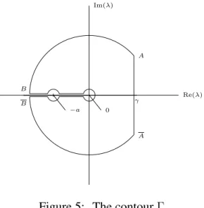
Lemma B.1 ( [45]). For 𝑘, 𝑑 > 0, ℒ−1 (︂ 𝑒−𝑘√𝑠 (𝑠 − 𝑑)√𝑠 )︂ = 𝑒 𝑑𝑡 2√𝑑𝑒 −𝑘√𝑑 erfc (︂ 𝑘 2√𝑡 − √ 𝑑𝑡 )︂ − 𝑒 𝑑𝑡 2√𝑑𝑒 𝑘√𝑑 erfc (︂ 𝑘 2√𝑡 + √ 𝑑𝑡 )︂ . Lemma B.2. For 𝑎 ∈ R, ℒ−1(︁√𝑎 + 𝑠𝑒− √ 𝑠 𝑦)︁(𝑡, 𝑦) = 1 𝜋 ∫︁ 𝑎 0 sin(𝑦√𝑟)√𝑎 − 𝑟 𝑒−𝑟𝑡d𝑟 − 1 𝜋 ∫︁ +∞ 0 cos(𝑦√𝑟 + 𝑎)√𝑟 𝑒−(𝑟+𝑎)𝑡d𝑟.
Proof. Inspired by [51], we use the Bromwich formula with the contour Γ illustrated in Figure 5. Since the integrals on the outer and inner arcs as well as half-circles are null,
ℒ−1(︁√𝑎 + 𝑠 𝑒− √ 𝑠 𝑦)︁(𝑟, 𝑦) = 1 2𝑖𝜋 ∫︁ 𝛾+𝑖∞ 𝛾−𝑖∞ √ 𝑎 + 𝑠 𝑒−𝑦 √ 𝑠𝑒𝑠𝑡d𝑠 = 1 2𝑖𝜋 (︂∫︁ 𝑎 0 (𝑒𝑖𝑦 √ 𝑟− 𝑒−𝑖𝑦√𝑟)√𝑎 − 𝑟 𝑒−𝑟𝑡 d𝑟 − ∫︁ +∞ 𝑎 (𝑒𝑖𝑦 √ 𝑟+ 𝑒−𝑖𝑦√𝑟) 𝑖√𝑟 − 𝑎 𝑒−𝑟𝑡 d𝑟 )︂ ,
and the result follows.
References
[1] M. Abramowitz and I. Stegun. Handbook of Mathematical Functions with Formulas, Graphs and Mathematical Tables. Dover Publications, ninth edition, 1970.
[2] T. Appuhamillage, V. Bokil, E. Thomann, E. Waymire, and B. Wood. Occupation and local times for skew Brownian motion with applications to dispersion across an interface. Ann. Appl. Probab., 21(1):183–214, 2011.
[3] T. Appuhamillage, V. Bokil, E. Thomann, E. Waymire, and B. Wood. Occupation and local times for skew Brownian motion with applications to dispersion across an interface. Ann. Appl. Probab., 21(5):2050–2051, 2011.