HAL Id: hal-02902171
https://hal.archives-ouvertes.fr/hal-02902171
Submitted on 17 Jul 2020
HAL is a multi-disciplinary open access
archive for the deposit and dissemination of
sci-entific research documents, whether they are
pub-lished or not. The documents may come from
teaching and research institutions in France or
abroad, or from public or private research centers.
L’archive ouverte pluridisciplinaire HAL, est
destinée au dépôt et à la diffusion de documents
scientifiques de niveau recherche, publiés ou non,
émanant des établissements d’enseignement et de
recherche français ou étrangers, des laboratoires
publics ou privés.
Distributed under a Creative Commons Attribution| 4.0 International License
K-Stacker: an algorithm to hack the orbital parameters
of planets hidden in high-contrast imaging
H. Le Coroller, M. Nowak, P. Delorme, G. Chauvin, R. Gratton, M. Devinat,
J. Bec-Canet, A. Schneeberger, D. Estevez, L. Arnold, et al.
To cite this version:
H. Le Coroller, M. Nowak, P. Delorme, G. Chauvin, R. Gratton, et al.. K-Stacker: an algorithm
to hack the orbital parameters of planets hidden in high-contrast imaging: First applications to
VLT/SPHERE multi-epoch observations. Astronomy and Astrophysics - A&A, EDP Sciences, 2020,
639, pp.A113. �10.1051/0004-6361/202037605�. �hal-02902171�
Astronomy
&
Astrophysics
https://doi.org/10.1051/0004-6361/202037605© H. Le Coroller et al. 2020
K-Stacker: an algorithm to hack the orbital parameters of planets
hidden in high-contrast imaging
First applications to VLT/SPHERE multi-epoch observations
?
H. Le Coroller
1, M. Nowak
2,3, P. Delorme
4, G. Chauvin
4, R. Gratton
5, M. Devinat
1, J. Bec-Canet
1,
A. Schneeberger
1, D. Estevez
6, L. Arnold
7, H. Beust
4, M. Bonnefoy
4, A. Boccaletti
8, C. Desgrange
9,10, S. Desidera
5,
R. Galicher
8, A. M. Lagrange
4, M. Langlois
11, A. L. Maire
12, F. Menard
4, P. Vernazza
1, A. Vigan
1, A. Zurlo
10,13,1,
T. Fenouillet
1, J. C. Lambert
1, M. Bonavita
5, A. Cheetham
14, V. D’orazi
5, M. Feldt
15,16, M. Janson
15, R. Ligi
17,
D. Mesa
5, M. Meyer
18, M. Samland
15,16, E. Sissa
5, J.-L. Beuzit
1, K. Dohlen
1, T. Fusco
19, D. Le Mignant
1, D. Mouillet
4,
J. Ramos
15, S. Rochat
4, and J. F. Sauvage
19(Affiliations can be found after the references)
Received 28 January 2020 / Accepted 21 April 2020
ABSTRACT
Context. Recent high-contrast imaging surveys, using the Spectro-Polarimetic High contrast imager for Exoplanets REsearch
(SPHERE) or the Gemini Planet Imager in search of planets in young, nearby systems, have shown evidence of a small number of giant planets at relatively large separation beyond 10–30 au, where those surveys are the most sensitive. Access to smaller physical separations between 5 and 30 au is the next step for future planet imagers on 10 m telescopes and the next generation of extremely large telescopes in order to bridge the gap with indirect techniques such as radial velocity, transit, and soon astrometry with Gaia. In addition to new technologies and instruments, the development of innovative observing strategies combined with optimized data processing tools is participating in the improvement of detection capabilities at very close angular separation. In that context, we recently proposed a new algorithm, Keplerian-Stacker, which combines multiple observations acquired at different epochs and takes into account the orbital motion of a potential planet present in the images to boost the ultimate detection limit. We showed that this algorithm is able to find planets in time series of simulated images of the SPHERE InfraRed Dual-band Imager and Spectrograph (IRDIS) even when a planet remains undetected at one epoch.
Aims. Our goal is to test and validate the K-Stacker algorithm performances on real SPHERE datasets to demonstrate the resilience of
this algorithm to instrumental speckles and the gain offered in terms of true detection. This will motivate future dedicated multi-epoch observation campaigns of well-chosen, young, nearby systems and very nearby stars carefully selected to search for planets in emitted and reflected light, respectively, to open a new path concerning the observing strategy used with current and future planet imagers.
Methods. To test K-Stacker, we injected fake planets and scanned the low signal-to-noise ratio (S/N) regime in a series of raw
observa-tions obtained by the SPHERE/IRDIS instrument in the course of the SPHERE High-contrast ImagiNg survey for Exoplanets. We also considered the cases of two specific targets intensively monitored during this campaign: β Pictoris and HD 95086. For each target and epoch, the data were reduced using standard angular differential imaging processing techniques and then recombined with K-Stacker to recover the fake planetary signals. In addition, the known exoplanets β Pictoris b and HD 95086 b previously identified at lower S/N in single epochs have also been recovered by K-Stacker.
Results. We show that K-Stacker achieves a high success rate of ≈100% when the S/N of the planet in the stacked image reaches
≈9. The improvement of the S/N is given as the square root of the total exposure time contained in the data being combined. At S/N < 6−7, the number of false positives is high near the coronagraphic mask, but a chromatic study or astrophysical criteria can help to disentangle between a bright speckle and a true detection. During the blind test and the redetection of HD 95086 b, and β Pic b, we highlight the ability of K-Stacker to find orbital solutions consistent with those derived by the current Markov chain Monte Carlo orbital fitting techniques. This confirms that in addition to the detection gain, K-Stacker offers the opportunity to characterize the most probable orbital solutions of the exoplanets recovered at low S/N.
Key words. planets and satellites: dynamical evolution and stability – methods: data analysis – instrumentation: adaptive optics – instrumentation: high angular resolution – stars: individual: β Pictoris – stars: individual: HD 95086
1. Introduction
Most of the 4100 exoplanets detected to date have been found using indirect methods, such as the radial velocity technique and photometric transits. It is indeed extremely difficult to detect
?Based on observations collected at the European Southern
Obser-vatory under programs: 095.C-0298, 096.C-0241, 097.C-0865, 198.C-0209, 099.C-0127.
planet light that is drowned in the much brighter diffracted light from its host star. Jupiter and Earth like planets are about 108to
1010fainter than their parent star in the visible band.
However, owing to a combination of eXtreme Adaptive Optics (ExAO), innovative coronagraphs, differential imaging, and sophisticated post-processing algorithms, direct imaging instruments have been able to detect and characterize young giant planets at large separation (>∼10 au). Across two decades
A113, page 1 of12 Open Access article,published by EDP Sciences, under the terms of the Creative Commons Attribution License (http://creativecommons.org/licenses/by/4.0),
of exoplanetary science in direct imaging, dozens of dedi-cated surveys have been carried out around young, nearby stars (Chauvin 2018b). These have led to the discovery of the first planetary mass companions in the early 2000s at large distances of ≥100 au. The implementation of differential techniques, start-ing in 2005, enabled the breakthrough discoveries of closer and lighter planetary mass companions such as HR 8799 bcde (10, 10, 10, and 7 MJupat 14, 24, 38, and 68 au, respectively;Marois et al. 2008,2010), β Pictoris b (8 MJupat 8 au;Lagrange et al. 2009), Fomalhaut b (<1 MJupat 177 au;Kalas et al. 2008; still
debated), HD 95086 b (5 MJupat 52 au;Rameau et al. 2013).
The current generation of ExAO planet imagers (Macintosh et al. 2014; Jovanovic et al. 2015; Beuzit et al. 2019), Gemini Planet Imager (GPI), Subaru Coronagraphic Extreme Adaptive Optics (SCExAO), Spectro-Polarimetic High contrast imager for Exoplanets REsearch (SPHERE) are now equipped with inte-gral field spectrographs offering exquisite near-infrared spectra of young giant planets to unveil the physical processes at play in their atmospheres and a link to their mechanisms of forma-tion. For the first time, these instruments have reached a contrast level of ≈10−5at a separation of about 200 to 900 mas, enabling
the detection of the new young planets 51 Eri b (2 MJupat 13 au; Macintosh et al. 2015), HIP 65426 b (9 MJupat 92 au;Chauvin et al. 2017b), and PDS 70 b (9 MJupat 29 au;Keppler et al. 2018).
An important finding from these high-contrast imaging surveys in recent years has been the low occurrence rate of giant planets beyond 30 au (0.6+0.7
−0.5%; see Bowler 2016).
Today, the Gemini Planet Imager Exoplanet Survey (GPIES) and the SPHERE High-contrast ImagiNg survey for Exoplan-ets (SHINE) large surveys of about 600 observed stars indicate that this scarcity extends down to 10 au (Nielsen et al. 2019;
Vigan et al. 2020), suggesting that the bulk of the giant planet population is typically located between 1 au and 10 au.
A prime goal of the future surveys will also be to bridge the gap with indirect techniques by imaging young Jupiters down to the snowline at about 3–5 au, depending on stellar type. The next generation of instruments such as SPHERE+ (Boccaletti et al. 2020) aim to reach contrasts of at least 10−5at ≈100 mas,
which represents an improvement of a factor of 3 in terms of angular separation with respect to SPHERE (Beuzit et al. 2019). K-Stacker, together with the SPHERE+ capability, has the poten-tial to achieve the core of the Jupiter-mass planets population at ≈3 au (i.e., ≈10−6 at ≈60 mas) in 10−100 h of exposure time,
by providing an additional factor of 3−10 in contrast. In terms of observing strategy, for planets at less than 10 au from a star at 10 pc to 20 pc, the orbital motion becomes comparable to the width of a 10 m telescope diffraction-limited Point Spread Function (PSF) in about 30 days. Taking into account observ-ing constraints and weather statistics because higher contrast can only be reached during the best nights with a seeing <0.600,
mul-tiple observations of very interesting young, nearby systems are usually spread over several days, months, and years (see case of β Pictoris; Lagrange et al. 2019a). In this case, the orbital motion of the potential planets makes a simple co-addition of the different images suboptimal in terms of pure detection, if not impossible.
The Keplerian motion of the planet has to be taken into account during the combination. On the Extremely Large Tele-scopes (ELTs), the situation will be even worse. The Point Spread Function (PSF) will be four to five times smaller than with the 10 m telescope class such as Very Large Telescope (VLT), Keck, Gemini, Subaru, Large Binocular Telescope (LBT), etc. These ELTs will be used to search for planets at very small separations (below 10 au) with first-light instruments (Chauvin 2018a). In
this case, the Keplerian motion could become non-negligeable in a matter of only a few days (Males et al. 2013).
Following similar principles previously applied to the search of new moons in solar systems such as Hippocamp, the seventh innermost moon of Neptune (Showalter et al. 2019), the Keplerian-Stacker (K-Stacker) algorithm described by
Le Coroller et al.(2015) is an observing strategy and method of data reduction applied to nearby stars. This technique consists in combining high-contrast images recorded during different nights, accounting for the orbital motion of the putative planet that we are looking for. Even if an individual image does not reveal the planet, we showed that an optimization algorithm like K-Stacker can be used to properly align the images according to Keplerian motion; for instance, 10–50 images taken over the course of several months or years. The resulting gain in signal-to-noise ratio (S/N) can allow for the detection of planets that are otherwise unreachable. This method can be used in addition to angular differential imaging (ADI) and spectral differential imaging (SDI) techniques (Racine et al. 1999;Marois et al. 2006) or any other high-contrast data reduction method designed to further improve the global detection limit. As a byproduct of the optimization algorithm, K-Stacker also directly provides the orbital parameters of the detected planets.
Ultimately, the main goal of K-Stacker would be to directly drive the observing strategy and scheduling of current and future planet imagers in which exposures would be split over sev-eral nights to maximize the detection performances. In PaperI
(Nowak et al. 2018), using simulated VLT-SPHERE observa-tions, we have shown that when the total number n of available images is large enough to get √n × (S/N) ≥ 7 (where (S/N) is the signal-to-noise levels in individual frames), the K-Stacker algo-rithm is able to detect the planet with a high level of reliability >90%. The number of false positives were low but the simulated images did not reproduce instrumental speckle noise and angu-lar spectral differential imaging (ASDI) reductions. The main goal of this paper is to validate the K-Stacker algorithm on real data obtained on sky reduced by the most recent ADI and ASDI Principal Component Analysis (PCA) algorithms.
In Sect.2, we describe the observations used in this paper, which come from the SPHERE SHINE survey (Chauvin et al. 2017a). In Sect.3, we present the results of a blind test in which K-Stacker was used to search for fake planets hidden in real InfraRed Dual-band Imager and Spectrograph (IRDIS) obser-vations reduced by a PCA ADI algorithm. We also study the capability of K-Stacker to recover the correct orbital parame-ters despite the typical errors encountered in real data, such as instrumental true north offsets or stellar mass and distance uncer-tainties. In Sect.4, we show that K-Stacker is able to recover the known companions β Pictoris b and HD 95086 b and show that the orbital parameters retrieved by K-Stacker are in agreement with the values found in the literature. We present in Sect. 5
the first K-Stacker searches for new planets around HD 95086 and β Pictoris, two targets which have been repeatedly observed during the SHINE survey. In Sect. 6, we discuss the strat-egy of future K-Stacker observations. Section7gives our final conclusions.
2. Description of the observations used in this paper
All the observations used in this paper come from the SHINE survey done with the Spectro-Polarimetic High contrast imager for Exoplanets REsearch (SPHERE) instrument at the focal plane of the VLT-UT3 (Beuzit et al. 2019). The SHINE program
(Chauvin et al. 2017b) is a very high-contrast near-infrared survey of more than 600 young, nearby stars aimed at search-ing for and characterizsearch-ing new planetary systems. The goal of this project is also to find statistical constraints on the rate, mass, and orbital distributions of the giant planet population at large orbits. Even if the SHINE observations were not organized for the K-Stacker “philosophy”, in which we plan to observe fewer stars but over more epochs, the number of observed targets reduced homogeneously by the SPHERE Data Center (Delorme et al. 2017;Galicher et al. 2018) allow us to test K-Stacker for the first time in real conditions.
The SPHERE instrument includes an extreme adaptive optics system, several types of coronagraphs, and three subsystems: IRDIS, the Integral Field Spectrograph (IFS), and the Zurich Imaging POLarimeter (ZIMPOL). In this paper we use observa-tions coming from IFS and IRDIS, which were designed to cover the near-infrared range for an efficient search of young planets (Beuzit et al. 2019). In the SHINE survey, two Apodized Lyot Coronagraphs (ALC) configurations were used: APO1-ALC2 (N-ALC-YJH-S) coronagraph with a focal plane mask of a diam-eter of 185 mas and the APO1-ALC3 (N-ALC-Ks) coronagraph with a focal plane mask of a diameter of 240 mas optimized for the IRDIFS and IRDIFS-EXT modes, respectively (Beuzit et al. 2019). In these modes, IRDIS and IFS work simultane-ously (Claudi et al. 2008;Zurlo et al. 2014) and IRDIS is used in a dual band imaging configuration (Dohlen et al. 2008;Vigan et al. 2010).
All the IRDIS observations used in the blind test described in Sect.3were acquired using the APO1-ALC2 coronagraph. In Sects.4and5, we also use the observations on two emblematic stars HD95086 and β Pictoris that have been observed regularly in the SHINE survey using the APO1-ALC2 and ALC3 coron-agraph (see TableB.1) to constrain the orbital parameters of the known planets b around these targets.
3. K-Stacker computation on real SHINE data
3.1. Setup of the blind test
In order to extend the demonstration of the K-Stacker algorithm on simulated IRDIS datasets presented in PaperI, we performed a new analysis on real IRDIS observations obtained during the SHINE survey. The methodology followed during this new blind experiment is similar to the approach discussed in PaperI, with the exception of an additional PCA ADI reduction step. To stay as close as possible to the conditions of PaperIand to demon-strate the true potential of K-Stacker, we injected planets in fake “K-Stacker runs”, each made of ten observations taken from the SHINE survey. As most stars have not been observed that many times during the survey, we created the K-Stacker runs by com-bining observations acquired on different but similar targets. In particular, we were careful in selecting observations of stars with similar magnitudes, and acquired in similar conditions such as seeing and adaptive optics (AO) performances. We created a total of five such fake K-Stacker runs, using a total of 50 different images from the survey.
Fake planets were then injected in the raw observations of each run by doing the following:
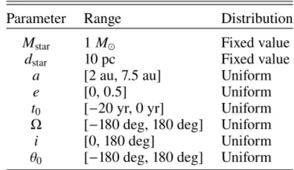
1. Randomly draw one run in which no planet is injected. 2. For each of the four other runs, draw a set of random orbital parameters (see Table1for an overview of orbital laws used), and inject the planet in each raw observation of the run according to the orbit drawn. The target star is assumed to have a mass of 1 M , and to be located at 10 pc. The planet
Table 1. Parameters used to inject the planet in the 30 K-Stacker runs of 10 observations of our blind experiment.
Parameter Range Distribution Mstar 1 M Fixed value
dstar 10 pc Fixed value
a [2 au, 7.5 au] Uniform
e [0, 0.5] Uniform
t0 [−20 yr, 0 yr] Uniform
Ω [−180 deg, 180 deg] Uniform i [0, 180 deg] Uniform θ0 [−180 deg, 180 deg] Uniform
Notes. The same ranges are used as in PaperI.
is injected at a random contrast uniformly drawn in the range [5 × 10−6,4 × 10−7].
3. Reduce each observation of each run using the PCA ADI tools of the SPHERE Data Center (Delorme et al. 2017;Galicher et al. 2018).
The process was repeated six times to create a total of 30 fake K-Stacker runs, in which 6 have no planets, and 24 have a planet injected randomly. The resulting runs were then classified based on the perfectly recombined (S/N)tot of the injected fake
plan-ets. We note that the S/N definition when using K-Stacker can be confusing, as we need to distinguish three different values: the S/N in each individual ADI observation of the run (simply S/N), the S/N after the K-Stacker recombination (S/N)KS, and the
opti-mal S/N that could be achieved if the orbit was perfectly known, and the images perfectly recombined (S/N)tot. The 30 runs were
then divided into the following three groups:
– Group I: composed of 13 runs for which (S/N)tot <2 for
the injected fake planets (or non injected fake planets). These planets can be considered as undetectable, that is, equivalent to no planet injected.
– Group II: composed of 9 runs for which 2 < (S/N)tot<12
for the injected fake planets (low-S/N regime)
– Group III: composed of 8 runs for which (S/N)tot>12 for
the injected fake planets and therefore easily detectable. 3.2. Blind check
Following the principles of PaperI, after running the K-Stacker algorithm, we asked an independent observer, who was not aware of the presence or not of fake planets in the images, the injec-tion phase, the S/N, or the orbital parameters, to check the final K-stacker recombined solutions and to assign for each run one of the three flags: “no detection”, “planet candidate”, and “possible candidate, more observations required”.
Among the 13 sets of Group I (i.e., (S/N)tot <2), 8 were
correctly flagged by the observer as no detection (i.e., true negatives); the five other solutions were flagged as “possible can-didates, more observations needed”. Because of the nature of the blind test performed, in which the same limited number of high-contrast observations were used multiple times, all the runs are not fully independent, and these five cases correspond to two truly independent candidates emerging from the noise. The typ-ical K-Stacker S/N for these five cases was (S/N)KS ≈ 6, and
although the observer did not claim a detection from these runs, in reality, they would probably have led to more observation time being spent on the targets. We consider these two cases as false positives.
0 2 4 6 8 10 12 14
S/N ratio (assuming perfect recombination)
0.0 0.5 1.0 1.5 2.0 2.5 3.0 3.5 4.0 Number of occurences False negatives True positives False positives
Fig. 1.Distribution of the planet candidates found and missed as a func-tion of the (S/N)tot given a perfect recombination of the images. The
true negatives, all grouped at S/N = 0, are not shown.
Among the nine runs of Group II (i.e., 2 < (S/N)tot <12),
five solutions were flagged as true detections by the observer and were indeed true positives. Two solutions at (S/N)tot =3.3
and (S/N)tot = 3.6 were found at (S/N)KS ≈ 6, and flagged by the observer as possible detections, with more observations required. These two solutions correspond to the same false pos-itives as described above. Two other solutions at (S/N)tot =3
and (S/N)tot =4 were flagged as no detection by the observer,
although the K-Stacker (S/N)KS was found to be between 7 and 8. In these two last cases, the orbits found by K-Stacker pass well at less than one pixel of the true positions of the fake planet in three images (epochs), but miss the planet along the other epochs. The contribution from the fake planet to the (S/N)KS explains the relatively high values obtained. We count these ambiguous cases as false negatives. Finally, all eight runs of Group III (i.e., (S/N)tot >12) were flagged by the observer as
detections and are indeed true positives.
In Fig.1, we report the histogram of the planets found and missed from Groups I and II. For clarity, solutions of Groups III with (S/N)tot > 12 are not shown. All these solutions with (S/N)tot>12 correspond to true positives. Even if the statistics
are poorer than in PaperI, we still find that K-Stacker is able to recover all the planets with (S/N)tot>6.5 i.e., S/N ' 2 in
indi-vidual observations. With only five truly independent runs of 10 observations used to create the 30 fake K-Stacker runs, it is dif-ficult to draw solid conclusions regarding the false positive rate. One of the two false alarms of Fig.1was found to be very close to the coronagraphic mask, where the false positive probability may be significantly higher (see also Sect.5). However, in every case, the observer did not claim a detection from the available observations, but merely suggested that the K-Stacker solution was possibly a planet and requested more observations.
3.3. Extracted orbital parameters
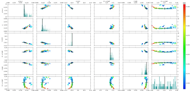
The result of the K-Stacker algorithm is a list of orbits sorted by S/N (see Paper Ifor detail). The S/N of the ≈50−100 first orbits is a relatively flat function before decreasing by steps (see example in Fig.2). For our study of the orbital parameters, we only kept the orbits before this drop in (S/N)KS (i.e., 68 first orbits in the example of Fig. 2). We checked that for the true positives of the SHINE blind test the first K-Stacker solutions before the decrease of (S/N)KSalways contained a set of orbital
parameters that pass well by the orbit of injection (see Fig.4). We show the orbital parameters in 2D maps (Fig.4) to be able
0 20 40 60 80 Orbit 0.08 0.07 0.06 0.05 0.04 0.03 0.02 0.01 0.00 SNR derivative
Evolution of the SNR derivative on the best 100 orbits
Fig. 2. K-Stacker (S/N)KS derivative in function of the orbit number
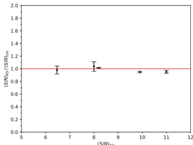
sorted by S/N. 5 6 7 8 9 10 11 12 (S/N)tot 0.0 0.2 0.4 0.6 0.8 1.0 1.2 1.4 1.6 1.8 2.0 (S /N )KS /(S /N )tot
Fig. 3.K-Stacker (S/N)KSdivided by (S/N)tot of a perfect
recombina-tion as a funcrecombina-tion of (S/N)tot.
to compare the K-Stacker solutions with the Markov chain Monte Carlo (MCMC) technique on the positions (Beust et al. 2016).
We also give a “mean” solution with its standard deviation (black cross in Fig.4). For all the planets detected by K-Stacker in the SHINE blind test (true positives in green of Fig.1), the mean solution of the orbital parameters is at maximum three standard deviations from the parameters of injection. This mean orbit always passes at less than ≈0.6 pixels from the true posi-tions of the fake planet in the images (see TableA.1). Figure3
shows also that the K-Stacker (S/N)KSfound with the mean
solu-tion of the orbital parameters is equal within the error bars to the (S/N)totof a perfect recombination. To conclude, K-Stacker has
recovered the orbital parameters well, although the planet has traveled over a maximum of 15−38% of its total orbital period (see Fig.4and TableA.1).
3.4. K-Stacker tolerances on the errors of real data
To limit the computation time, K-Stacker does not include true north error, or stellar mass and distance as free parameters. These values are fixed values set by the user. In this section, we inves-tigate the capability of K-Stacker to converge despite possible errors on these parameters.
3.4.1. Tolerance on the stellar mass error and impact on the orbital parameters
To test the robustness of K-Stacker to errors on the stellar mass, we performed an experiment, in which we kept the mass of the
Fig. 4.Example of orbital parameters coming from one true positive solution of the SHINE blind test (see Sect.3.2). In each subplot, each point corresponds to the parameters of one orbit found by K-Stacker with the color of its (S/N)KSvalue. In the diagonal, the histograms for each orbital
parameter are shown. The dark cross corresponds to the mean of the K-Stacker orbits. The size of the dark cross is 1σ of each orbital parameter. The star is at the position of the orbital parameters used to inject the fake planet.
target star to a fixed value M = 1 M when calculating the orbit
of the injected planets, but changed the mass used by K-Stacker to M + δM. For a circular face-on orbit of semimajor axis a, the orbital velocity is given by
Vorb= r GMa . (1)
Thus, a small error δM on the mass M of the star directly translates to an error δVorbon the velocity given by
δVorb= 12r Ga MδM1/2. (2)
This error on the orbital velocity leads to a K-Stacker estimate of the position in each image that “drifts” with time, compared to the real position of the planet. Assuming that the algorithm can always play on appropriate parameters to minimize the total error by properly aligning the center of the time series, we can calculate the typical mean position error ∆Xmeanfor a sequence
of N observations acquired at a regular time interval ∆T over a total period T = (N − 1)∆T as follows:
∆Xmean= 1 N k=N X k=1 k∆TδVorb=T 2δVorb. (3)
For a star at a distance d, the associated angular error is then ∆θmean=1 4 T d r G a δM M1/2, (4)
where d = 10 pc, T = 3 yr, a ' 5 au, and M = 1 M , an error
of 0.1 M on the mass of the star leads to a mean angular error
of 21 mas, similar to the size of the SPHERE PSF. For most of
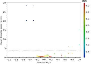
the stars of the SHINE survey the mass is known with an accu-racy better than 10% (Desidera et al. 2015), so the effect should remain limited. Nevertheless, to study the impact of this error on the performance of K-Stacker, we used the algorithm on a fake run while explicitly adding an error on the stellar mass. In Fig. 5, we give the mean distance between the solution found by K-Stacker and the injected position of the planet, as a func-tion of the error on the stellar mass δM. Interestingly, K-Stacker is able to tolerate a relatively large error on the stellar mass (−0.2 < δ M < 0.2), which should in principle lead to an error of more than a PSF on the position of the planet (see Eq. (4)). This could be explained by the fact that the algorithm somehow compensates for the wrong mass by altering some of the orbital parameters. Figure6, which gives the retrieved orbital parame-ters as a function of δM, indicates that both a and e are strongly correlated with δM, and thus that varying these parameters can indeed help to compensate for the error on the stellar mass.
Although this has not been studied in depth in this work, Fig.5indicates that K-Stacker can potentially be used to retrieve the mass of the central star together with the other parame-ters. The maximum S/N value of (S/N)KS=6.34 is obtained at
δM = 0 and, in the region of small mass errors (δM/M < 10%), the (S/N)KSfunction shows a clear drop of up to 0.2 to 0.4 when
departing from δM = 0, with no other apparent local maximum. The situation is more complicated for higher initial error on the mass, with a distinct secondary maximum of (S/N)KS around
δM = 0.2 M visible in Fig.5. The reason for the existence of
such a secondary maximum is not clear and the grid sampling could play an important role in this situation. Furthermore, it remains to be determined whether this apparent local maximum exists in the full parameter space, or if it is an effect of the projec-tion of the (S/N)KSfunction against δM only. A gradient descent
taking into account all the orbital parameters and the stellar mass simultaneously could potentially avoid this apparent secondary maximum. But this remains to be demonstrated, and a significant
1.0 0.8 0.6 0.4 0.2 0.0 0.2 0.4 0.6 0.8 1.0 mass (M ) 0 5 10 15 20 25 30
Mean distance error (pixels)
5.6 5.7 5.8 5.9 6.0 6.1 6.2 6.3
SNR
Fig. 5.Results of the K-Stacker algorithm when including an error on the stellar mass used by the algorithm to calculate the orbital positions at each epoch. The dots (resp. dashes) show the mean (resp. maximum) distance between the true position and the position found by K-Stacker in all the images as a function of the error on the mass. These dots are color coded to indicate the corresponding (S/N)KS. The black dashed
line indicates the size of the FWHM of the instrumental PSF (i.e., K-Stacker has missed the planet at least in one image when a small line is above the dashed line).
reworking of the algorithm is necessary to constrain the stellar mass on targets for which it is largely uncertain. This is out of scope of the current paper but could be considered, if necessary, for example in the case of low-mass stars for which the mass is not always well known.
3.4.2. Tolerance on the true north error
True north (TN) gives the absolute rotational orientation of observations. An error on the TN is responsible for a rotational misalignment between the different images used by K-Stacker, resulting in an apparent deviation of the planet motion from Keplerian orbits. For reference, the typical true north error in SPHERE, estimated using a well-defined observing strategy of a given astrometric field (Maire et al. 2016), does not exceed 0.1 deg. For NaCo, similar values of 0.1−0.2 deg were obtained over more than a decade (Chauvin et al. 2012,2015). To check the consequences of a TN error on the K-Stacker algorithm, we simulated several observations taking into account the real distri-bution of the TN errors measured on SPHERE (see TableA.2). The maximum TN error is 0.08 deg, with a standard deviation of 0.026 deg, which corresponds to 0.4 mas, or ≈1/100 of the full width at half maximum (FWHM) of the PSF at the edge of the area corrected for AO. At that level, this error should not affect the performance of K-Stacker in any noticeable way. Indeed, we find that K-Stacker has no problem recovering the planets, and gives the same final S/N and orbital parameters, even when multiplying the SPHERE TN errors by a factor of 10.
3.4.3. Tolerance on the stellar distance error
The stellar distances are known from the HIPPARCOS (van Leeuwen 2007) or Gaia missions (Luri et al. 2018). The typical error on the parallax given by Gaia Data Release 2 (Gaia DR2) for bright sources (mag < 14) is δ$ < 0.1 mas (Luri et al. 2018). For a star at 10 pc ($ = 100 mas), this translates to a relative error on the distance of δd/d = δ$/$ = 0.1%.
To determine the position of the possible planet in each image, K-Stacker first calculates the position of the planet around
0.20 0.15 0.10 0.05 0.00 0.05 0.10 0.15 0.20 mass (M ) 3 2 1 0 1 2 3
Err
or
on
w (
rad
)
0.20 0.15 0.10 0.05 0.00 0.05 0.10 0.15 0.20 1.5 1.0 0.5 0.0 0.5 1.0 1.5Err
or
on
i (r
ad)
0.20 0.15 0.10 0.05 0.00 0.05 0.10 0.15 0.20 3 2 1 0 1 2 3Err
or
on
(ra
d)
0.20 0.15 0.10 0.05 0.00 0.05 0.10 0.15 0.20 4 2 0 2 4Err
or
on
t0
(Yr
)
0.20 0.15 0.10 0.05 0.00 0.05 0.10 0.15 0.20 0.20 0.15 0.10 0.05 0.00 0.05 0.10 0.15 0.20Err
or
on
e
0.20 0.15 0.10 0.05 0.00 0.05 0.10 0.15 0.20 1.0 0.5 0.0 0.5 1.0Err
or
on
a (
a.u
.)
Fig. 6.Difference between the orbital parameters found by K-Stacker and the real values of injection, as a function of the error on the stellar mass.
its central star and then projects this position on the detector. The projected position is directly proportional to d−1. Given that the
corrected field for AO on SPHERE is typically 100, the
projec-tion error induced by a 0.1% error on the distance of the star can be at most 1 mas (i.e., much smaller than the instrumental PSF). Consequently, this error is negligible for K-Stacker.
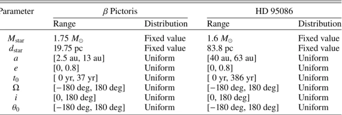
Table 2. Search space for the two K-Stacker runs on two targets of the SHINE survey.
Parameter βPictoris HD 95086
Range Distribution Range Distribution
Mstar 1.75 M Fixed value 1.6 M Fixed value
dstar 19.75 pc Fixed value 83.8 pc Fixed value
a [2.5 au, 13 au] Uniform [40 au, 63 au] Uniform
e [0, 0.8] Uniform [0, 0.8] Uniform
t0 [ 0 yr, 37 yr] Uniform [ 0 yr, 386 yr] Uniform
Ω [−180 deg, 180 deg] Uniform [−180 deg, 180 deg] Uniform
i [0, 180 deg] Uniform [0, 180 deg] Uniform
θ0 [−180 deg, 180 deg] Uniform [−180 deg, 180 deg] Uniform
Fig. 7.Best recombined image resulting from the K-Stacker run on β Pictoris. At each epoch, the images are rotated and shifted to put the planet on its periastron position found by K-Stacker, and the frames are co-added. The planet b is detected at a (S/N)KSlevel of 24.5.
4. Applying K-Stacker to known exoplanets
In this section, we present the first results obtained with K-Stacker on two real planets: β Pic b and HD 95086 b. Each of these emblematic objects has been observed multiple times with SPHERE during the SHINE survey, and together they provide a good test of K-Stacker in different conditions. β Pic b is on an edge-on orbit with a significant orbital motion. HD 95086 b is rather on pole-on configuration and has moved by only a few PSFs over the five years of IRDIS monitoring.
4.1. β Pic b
Eleven IFS observations of β Pictoris, spread over more than three years between 2015 and 2018, were available in the SHINE survey (Table B.1). We reduced these data with a PCA ASDI algorithm (Mesa et al. 2015). Although in this case, with a mean S/N of 7.42, the planet is clearly detected in each individual image, K-Stacker was set up to look blindly for planets in the range of orbital parameters given in Table2.
The planet β Pic b is detected at a total K-Stacker recombined (S/N)KS =24.5 (see Fig.7), a gain of a factor 3.3 compared to
the individual PCA ASDI reduced observations. For a set of 11 observations, this gain is optimal.
Table 3. Mean orbital solutions found by K-Stacker on the two targets of the SHINE survey presented in Sect.4of this paper.
Parameter Unit β Pictoris b HD 95086 b a au 9.37 ± 1.68 51.45 ± 4.66 e – 0.07 ± 0.12 0.16 ± 0.09 t0 yr 2.95 ± 4.78 −70.98 ± 55.01 Ω + θ0 rad 4.23 ± 1.89 1.89 ± 1.33 i rad 1.60 ± 0.11 0.63 ± 0.2 Ω− θ0 rad 0.95 ± 1.89 5.14 ± 1.5
Notes. The parameter t0 gives the time at periastron, counted from an
arbitrary reference date set at 01/12/2014 for β Pictoris and 05/05/2015 for HD 95086.
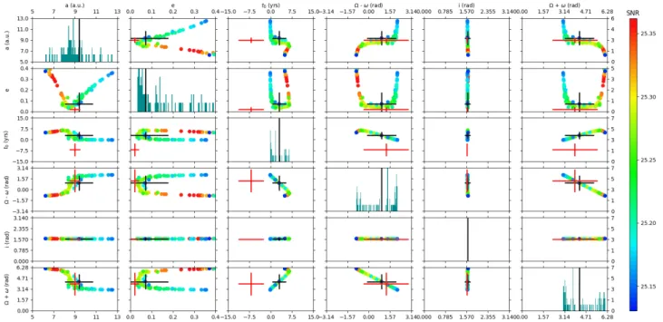
Figure 8 gives the distribution of the 89 best orbits found by K-Stacker in the parameter space. The black crosses on the different subplots give the position of the mean value of these 89 orbits, with the associated 1σ spread (see also Table3). For comparison, the red cross gives the best estimates and 1σ uncer-tainties fromLagrange et al.(2019a), converted to the reference system used in K-Stacker.
Since K-Stacker does not implement a proper MCMC explo-ration of the parameter space, the statistical meaning of the corner plots presented in Fig.8is not straightforward. But these pseudo-corner plots share some interesting similarities with the results of a more classical approach to fitting, as presented in
Lagrange et al. (2019a): a clear V-shaped correlation between the semi-major axis a and the eccentricity e, related to a degen-eracy on the position of periastron/apoastron; a well constrained edge-on inclination; and an eccentricity distribution that peaks at e < 0.1. Overall, the orbital solution resulting from the K-Stacker run is in good agreement with the recent results ofLagrange et al. (2019a). The only significant difference is on t0 found
by Lagrange et al.(2019a), which is near the apoastron of the K-Stacker mean solution (see red and dark crosses for t0 in
Fig.8). This ambiguity in the periastron/apoastron is reinforced by the small eccentricity and the incomplete coverage of the orbit. This will be solved with further monitoring.
4.2. HD 95086 b
For HD 95086, a total of eight observations are available in the SHINE survey between May 2015 and May 2019, and all of these were obtained in good conditions in the H part of the spectrum with IFS (see TableB.1). The data were reduced using a PCA ASDI algorithm.
Fig. 8.Histograms and 2D diagrams of the β Pictoris b orbital parameters found by K-Stacker. Left, top, and bottom: scale of the orbital param-eters. Right: scale of the histograms. 89 points in each 2D diagram corresponding to the 89 orbits with the highest (S/N)KSfound by K-Stacker.
The color of each point gives the (S/N)KSindicated at right. The dark cross indicates the mean value of the orbital parameters with their error bars.
The red cross shows the higher probability density found by an MCMC technique inLagrange et al.(2019a) converted in the K-Stacker referential. The origin of the t0K-Stacker date is the 01/12/2014.
Fig. 9. Best recombined image resulting from the K-Stacker run on HD 95086. At each epoch, the images are rotated and shifted to put the planet on its periastron position found by K-Stacker, and the frames are co-added. The planet b is detected at a (S/N)KSlevel of 9.97.
The algorithm was set to search for planets in the range of parameters given in Table2. The planet HD 95086 b is detected (Fig.9) at a recombined (S/N)KS =9.97. The mean S/N in the individual PCA ASDI reduced observations was 3.67. Thus, the S/N is improved by a factor 2.72 by K-Stacker. For a series of eight observations, this is again very close to the optimal case. The mean orbital solution found by K-Stacker is presented in Table3, and the associated pseudo-corner plot can be found in Fig. 10. Although 1.4% of the orbital period of HD 95086 b has been covered by the observations, the orbital parameters are relatively well constrained. Again, the pseudo-corner plots of
K-Stacker share some similarities with the results of a more clas-sical approach to fitting, as presented inChauvin et al.(2018). Within the error bars, the mean values of the orbital parameters found by K-Stacker (see dark and red crosses of Fig.10) are equal to the solutions coming from the MCMC technique described in
Chauvin et al.(2018).
5. Searching for inner exoplanets
In this Section, we focus on the search for additional inner plan-ets around HD 95086 and β Pictoris using the SHINE reduced data (TableB.1). Indeed, the presence of one or two additional inner giant planets is suspected considering the double-belt architecture of HD 95086 (Chauvin et al. 2018) and that a ∼9 MJupplanet β Pic c has been found using radial velocity, at
2.7 au from the star (Lagrange et al. 2019b). To search for addi-tional companions in these systems, we proceed using the same K-Stacker algorithm, in which we introduce an initial step of masking the known imaged planet b from the individual images. We search in the inner area of HD 95086 and β Pictoris with the parameters given in the Table4.
For both HD 95086 and β Pictoris, we find a bright sec-ondary feature, close to the coronagraphic mask (see Fig.11). For HD 95086, the feature is located at a = 16.7 au and has a low (S/N)KS =4.4. Its spread shape indicates a probable false positive, but a more detailled study will be done in a future work (Desgrange et al., in prep.) to try to determine if it is a true detection or not.
In the case of β Pictoris, the compact feature is found at (S/N)KS = 4.8 (Fig. 11) with the orbital parameters given at
Table 5. This solution is compatible with the orbital param-eters inferred from the following radial velocities (Lagrange et al. 2019b): a = 2.6948 au, e = 0.243, t0 = −7.87206 yr,
θ0=4.62 rad (where t0and θ0were expressed in the K-Stacker
Fig. 10. Histograms and 2D diagrams of the HD 95086 b orbital parameters found by K-Stacker. Left, top, and bottom: scale of the orbital parameters. Right: scale of the histograms. The 129 points in each 2D diagram correspond to the 129 orbits of the higher (S/N)KS found by
K-Stacker. The color of each point gives the (S/N)KSindicated at right. The dark cross indicates the mean value of the orbital parameters with their
error bars. The red cross shows the higher probability density found by an MCMC technique inChauvin et al.(2018) converted in the K-Stacker referential. The origin of the t0K-Stacker date is 05/05/2015.
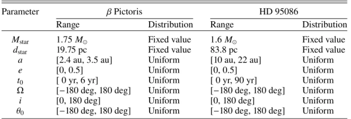
Table 4. Search space in the inner part of the two stars β Pictoris and HD 95086.
Parameter βPictoris HD 95086
Range Distribution Range Distribution
Mstar 1.75 M Fixed value 1.6 M Fixed value
dstar 19.75 pc Fixed value 83.8 pc Fixed value
a [2.4 au, 3.5 au] Uniform [10 au, 22 au] Uniform
e [0, 0.5] Uniform [0, 0.5] Uniform
t0 [ 0 yr, 6 yr] Uniform [ 0 yr, 90 yr] Uniform
Ω [−180 deg, 180 deg] Uniform [−180 deg, 180 deg] Uniform i [0, 180 deg] Uniform [0, 180 deg] Uniform θ0 [−180 deg, 180 deg] Uniform [−180 deg, 180 deg] Uniform
The semimajor axis found by K-Stacker is larger by 0.3 au but the PSF of the planet c is partially masked at several epochs by the coronagraphic mask and can therefore disturb the solution of K-Stacker. However, the parameters Ω = −2.0 rad ± 1.5 rad and i = +1.85 rad ± 0.86 rad give an orbit that is misaligned with the disk that is very difficult to explain from a dynamical point of view. In the blind test (Sect.3.2), we had two ambiguous cases in which the orbits found by K-Stacker passed well by the planet positions only at three to four epochs over 10. Thus, even if the orbit found by K-Stacker is not correct, a part of the light of this “bright” structure (Fig.11) could come from β Pictoris c. In all these cases, the probability of a true detection at (S/N)KS ≤ 5 is
smaller than 50%.
6. Strategy of future K-Stacker observations
A fundamental question for any potential future surveys with K-Stacker will be to select the optimum number of observations per target. The blind tests realized on simulated IRDIS images (Nowak et al. 2018) and on real data (see Sect.3) show that an (S/N)KS>7 must be reached to claim a true detection with high
Table 5. Orbital parameters of the solution found by K-Stacker in the inner part of β Pictoris.
Parameter Unit Values a au 3.0 ± 0.3 e – 0.14 ± 0.1 t0 yr −8.3 ± 0.8 Ω rad −2.0 ± 1.5 i rad +1.85 ± 0.86 θ0 rad +4.7 ± 1.5
confidence (i.e., small rate of false alarm). An S/N > 7 is also required to be able to do a precise spectral analysis and confirm a true detection by characterizing the physical properties of the planet (e.g., atmosphere composition, temperature, surface grav-ity, and clouds detections); see for example the characterization of the planets around the stars HR 8799, β Pic, HD 95086, 51Eri, HIP 65426, PDS 70 (Bonnefoy et al. 2016;Chilcote et al. 2017;
Beta pic
HD 95086
Fig. 11.Recombined images obtained with K-Stacker, when searching for additional companions around β Pictoris and HD 95086, two systems observed in the SHINE survey. At each epoch, the images are rotated and shifted to put the detection on its periastron position found by K-Stacker, and the frames are co-added. In each case, a bright spot can be seen near the coronagraphic mask (red arrow), which corresponds to the best solution found by the algorithm. In the case of β Pic, the corresponding (S/N)KSis 4.8. For HD 95086, the (S/N)KSis 4.4.
But, further work is required to develop a K-Stacker exoplanet statistical analysis tool: using a similar approach as with the multipurpose exoplanet simulation system (MESS) algorithm (Bonavita et al. 2012), we should be able to inject numerous fake planets in series of observations to compute a probability of detection in function of the planet mass by using model mass-luminosity relationships (Baraffe et al. 2003). This approach will allow us to give an upper mass limit for planets hidden in the data even when K-Stacker does not detect anything.
The total exposure time required for K-Stacker also depends on the number of observations already done. For example, to confirm the detection of β Pictoris c that has been found at (S/N)KS =4.8 in 11 exposures, a minimum of 11 ∗ [(7/4.8)2− 1] ≈ 12 new observations are needed to reach (S/N)KS ≈ 7. ; this
number of exposures could be slightly reduced by using radial velocity constraints to schedule the β Pictoris c observations when the planet is fully out of the coronagraphic mask.
Figure3and TableA.1shows that K-Stacker is able to recom-bine in a close to optimal way a series of observations with very different orbital parameters. Thus, in principle, the total S/N of a K-Stacker run should only depend on the total exposure time, and not on the number of individual exposures in which it is divided. In these conditions, better constraints on the orbital parameters could be obtained at fixed total exposure time by taking as many exposures over a period as long as possible. But, to reach higher contrast (i.e., per individual exposure and in the final K-Stacker recombined image), a minimum exposure time by observation is required to have enough field-of-view rotation for a good ADI substraction; that is, in each observation, a parallactic rotation of at least one PSF FWHM at the position of the planet must be reached to subtract the instrumental speckles with ADI effi-ciently. The trade-off comes from the difficulty in setting up the observation strategy, telescope overheads, and star declination (to adjust the minimum exposure of individual observations).
For future imaging surveys with K-Stacker on SPHERE+ (Boccaletti et al. 2020) and/or the ELTs instruments, a soft-ware to optimize observing schedules will have to be developed. Inspired from the algorithm used in the SHINE survey (Lagrange et al. 2016), the goal of this K-Stacker scheduler will be to
compute the minimum exposure time required at each epoch for each star to have an efficient ADI subtraction, but at the same time to split the observations over at least 10−20% of the orbital period of the searched planets to get accurate orbital parameters.
7. Conclusions
For the first time, we tested the K-Stacker algorithm on real IRDIS and IFS observations, reduced with the PCA ADI and ASDI algorithms, in a similar fashion as in the SHINE sur-vey. From a blind experiment, in which planets are injected on random orbits in the images before the PCA ADI reduc-tion and recovered by the K-Stacker algorithm, we conclude that the detection statistics are similar to what was previously obtained with simulated non-ADI reduced images: the suc-cess rate is close to 100% when searching for companions for which the recombined (S/N)KS' 9, and it drops significantly at
(S/N)KS' 5.
Using data on two targets repeatedly observed during the SHINE survey (β Pic, observed 11 times; HD 95086, observed 8 times), we have shown that the K-Stacker algorithm is good at recovering the known companions β Pic b and HD 95086 b. K-Stacker also provides orbital parameter estimates in agreement with current literature values. The gain provided by K-Stacker recombination is very close to the square root of the number of observations combined (i.e., close to optimal).
We also searched for additional substellar companions around these two stars. We found two bright features, corre-sponding to two possible planets orbiting within the orbit of the known companions. However, these two features are found at low (S/N)KS where it is difficult to reach a conclusion concerning
a true detection or not. A dedicated analysis will be done on the peak found around HD 95086 in a future work (Desgrange et al., in prep.). The c candidate detected by K-Stacker around β Pictoris without using prior information from the radial veloc-ity detection of β Pictoris c is on a trajectory compatible with the orbital parameters found byLagrange et al.(2019b). But, the K-Stacker orbit is misaligned with the disk and the (S/N)KS≈ 5
the relatively large error bars on the euler angles (Ω, i, θ0) the
1−σ agreement between the putative K-stacker detection and the radial velocity solution is encouraging and more observations are required to constrain the orbital parameters and to deter-mine if at least a part of the light of this detection comes from βPictoris c.
Acknowledgements. SPHERE is an instrument designed and built by a consor-tium consisting of IPAG (Grenoble, France), MPIA (Heidelberg, Germany), LAM (Marseille, France), LESIA (Paris, France), Laboratoire Lagrange (Nice, France), INAF–Osservatorio di Padova (Italy), Observatoire de Genève (Switzerland), ETH Zurich (Switzerland), NOVA (Netherlands), ONERA (France) and ASTRON (Netherlands) in collaboration with ESO. SPHERE was funded by ESO, with additional contributions from CNRS (France), MPIA (Germany), INAF (Italy), FINES (Switzerland) and NOVA (Netherlands). SPHERE also received funding from the European Commission Sixth and Seventh Framework Programmes as part of the Optical Infrared Coordination Network for Astronomy (OPTICON) under grant number RII3-Ct-2004-001566 for FP6 (2004–2008), grant number 226604 for FP7 (2009–2012) and grant num-ber 312430 for FP7 (2013–2016). We also acknowledge financial support from the Programme National de Planétologie (PNP) and the Programme National de Physique Stellaire (PNPS) of CNRS-INSU in France. This work has also been supported by a grant from the French Labex OSUG@2020 (Investissements d’avenir – ANR10 LABX56). The project is supported by CNRS, by the Agence Nationale de la Recherche (ANR-14-CE33-0018). It has also been carried out within the frame of the National Centre for Competence in Research PlanetS sup-ported by the Swiss National Science Foundation (SNSF). M.R.M., H.M.S., and S.D. are pleased to acknowledge this financial support of the SNSF. Finally, this work has made use of the SPHERE Data Centre, jointly operated by OSUG/IPAG (Grenoble), PYTHEAS/LAM/CESAM (Marseille), OCA/Lagrange (Nice), Observatoire de Paris/LESIA (Paris), and Observatoire de Lyon, also sup-ported by a grant from Labex OSUG@2020 (Investissements d’avenir – ANR10 LABX56). We thank P. Delorme and E. Lagadec (SPHERE Data Centre) for their efficient help during the data reduction process. This research has made use of computing facilities operated by CeSAM data center at LAM, Marseille, France.
References
Baraffe, I., Chabrier, G., Barman, T. S., Allard, F., & Hauschildt, P. H. 2003, A&A, 402, 701
Beust, H., Bonnefoy, M., Maire, A. L., et al. 2016,A&A, 587, A89 Beuzit, J. L., Vigan, A., Mouillet, D., et al. 2019,A&A, 631, A155
Boccaletti, A., Chauvin, G., Mouillet, D., et al. 2020, ArXiv e-prints [arXiv:2003.05714]
Bonavita, M., Chauvin, G., Desidera, S., et al. 2012,A&A, 537, A67 Bonnefoy, M., Zurlo, A., Baudino, J. L., et al. 2016,A&A, 587, A58 Bowler, B. P. 2016,PASP, 128, 102001
Chauvin, G. 2018a, ArXiv e-prints [arXiv:1810.02031] Chauvin, G. 2018b,SPIE Conf. Ser., 10703, 1070305
Chauvin, G., Lagrange, A. M., Beust, H., et al. 2012,A&A, 542, A41 Chauvin, G., Vigan, A., Bonnefoy, M., et al. 2015,A&A, 573, A127
Chauvin, G., Desidera, S., Lagrange, A.-M., et al. 2017a, in SF2A-2017: Pro-ceedings of the Annual meeting of the French Society of Astronomy and Astrophysics, eds. C. Reylé, P. Di Matteo, F. Herpin, et al., 331
Chauvin, G., Desidera, S., Lagrange, A.-M., et al. 2017b,A&A, 605, L9 Chauvin, G., Gratton, R., Bonnefoy, M., et al. 2018,A&A, 617, A76 Chilcote, J., Pueyo, L., De Rosa, R. J., et al. 2017,AJ, 153, 182
Claudi, R., Beuzit, J. L., Feldt, M., et al. 2008, in European Planetary Science Congress 2008, 875
De Rosa, R. J., Rameau, J., Patience, J., et al. 2016,ApJ, 824, 121
Delorme, P., Meunier, N., Albert, D., et al. 2017, in SF2A-2017: Proceedings of the Annual meeting of the French Society of Astronomy and Astrophysics, eds. C. Reylé, P. Di Matteo, F. Herpin, et al., 347
Desidera, S., Covino, E., Messina, S., et al. 2015,A&A, 573, A126 Dohlen, K., Saisse, M., Origne, A., et al. 2008,SPIE Conf. Ser., 7018, 59 Galicher, R., Boccaletti, A., Mesa, D., et al. 2018,A&A, 615, A92 Jovanovic, N., Martinache, F., Guyon, O., et al. 2015,PASP, 127, 890 Kalas, P., Graham, J. R., Chiang, E., et al. 2008,Science, 322, 1345 Keppler, M., Benisty, M., Müller, A., et al. 2018,A&A, 617, A44 Lagrange, A.-M., Kasper, M., Boccaletti, A., et al. 2009,A&A, 506, 927 Lagrange, A.-M., Rubini, P., Brauner-Vettier, N., et al. 2016,SPIE Conf. Ser.,
9910, 991033
Lagrange, A. M., Boccaletti, A., Langlois, M., et al. 2019a, A&A, 621, L8
Lagrange, A. M., Meunier, N., Rubini, P., et al. 2019b,Nat. Astron., 3, 1135 Le Coroller, H., Nowak, M., Arnold, L., et al. 2015, in Proceedings of colloquium
Twenty years of giant exoplanets held at Observatoire de Haute Provence, France, October 5, eds. I. Boisse, O. Demangeon, F. Bouchy, & L. Arnold, 59 Luri, X., Brown, A. G. A., Sarro, L. M., et al. 2018,A&A, 616, A9
Macintosh, B., Graham, J. R., Ingraham, P., et al. 2014,Proc. Natl. Acad. Sci., 111, 12661
Macintosh, B., Graham, J. R., Barman, T., et al. 2015,Science, 350, 64 Maire, A.-L., Langlois, M., Dohlen, K., et al. 2016,SPIE Conf. Ser., 9908,
990834
Males, J. R., Skemer, A. J., & Close, L. M. 2013,ApJ, 771, 10
Marois, C., Lafrenière, D., Doyon, R., Macintosh, B., & Nadeau, D. 2006,ApJ, 641, 556
Marois, C., Macintosh, B., Barman, T., et al. 2008,Science, 322, 1348 Marois, C., Zuckerman, B., Konopacky, Q. M., Macintosh, B., & Barman, T.
2010,Nature, 468, 1080
Mesa, D., Gratton, R., Zurlo, A., et al. 2015,A&A, 576, A121 Müller, A., Keppler, M., Henning, T., et al. 2018,A&A, 617, L2 Nielsen, E. L., De Rosa, R. J., Macintosh, B., et al. 2019,AJ, 158, 13 Nowak, M., Le Coroller, H., Arnold, L., et al. 2018,A&A, 615, A144
Racine, R., Walker, G. A. H., Nadeau, D., Doyon, R., & Marois, C. 1999,PASP, 111, 587
Rameau, J., Chauvin, G., Lagrange, A.-M., et al. 2013,ApJ, 779, L26 Showalter, M. R., de Pater, I., Lissauer, J. J., & French, R. S. 2019,Nature, 566,
350
van Leeuwen, F. 2007,A&A, 474, 653
Vigan, A., Moutou, C., Langlois, M., et al. 2010,MNRAS, 407, 71 Vigan, A., Fontanive, C., Meyer, M., et al. 2020,A&A, submitted Zurlo, A., Vigan, A., Mesa, D., et al. 2014,A&A, 572, A85
1 Aix Marseille Univ., CNRS, CNES, LAM, Marseille, France
e-mail: [email protected]
2 Institute of Astronomy, University of Cambridge, Madingley Road,
Cambridge CB3 0HA, UK
3 Kavli Institute for Cosmology, University of Cambridge, Madingley
Road, Cambridge CB3 0HA, UK
4 Univ. Grenoble-Alpes, CNRS, IPAG, 38000 Grenoble, France 5 INAF – Osservatorio Astronomico di Padova, Vicolo
dell’Osservatorio 5, 35122 Padova, Italy
6 LAPP UMR5814, 9 chemin de Bellevue BP 110 Annecy-le-Vieux
74941 Annecy Cedex, France
7 CFHT Corporation, 65-1238 Mamalahoa Hwy, Kamuela, Hawaii
96743, USA
8 LESIA, Observatoire de Paris, CNRS, University Pierre et Marie
Curie Paris 6 and University Denis Diderot Paris 7, 5 place Jules Janssen, 92195 Meudon, France
9 Univ. Lyon, ENS de Lyon, Univ. Lyon1, Lyon, France
10 Núcleo de Astronomía, Facultad de Ingeniería y Ciencias,
Universi-dad Diego Portales, Av. Ejercito 441, Santiago, Chile
11 CRAL, UMR 5574, CNRS, Université Lyon 1, 9 avenue Charles
André, 69561 Saint Genis Laval Cedex, France
12 STAR Institute/Université de Liège, Allée du Six Août 19c, 4000
Liège, Belgium
13 Facultad de Ingeniería y Ciencias, Universidad Diego Portales, Av.
Ejercito 441, Santiago, Chile
14 Geneva Observatory, University of Geneva, Chemin des Maillettes
51, 1290 Versoix, Switzerland
15 Max-Planck-Institut für Astronomie, Königstuhl 17, 69117
Heidelberg, Germany
16 Department of Astronomy, Stockholm University, AlbaNova
University Center, 10691 Stockholm, Sweden
17 INAF-Osservatorio Astronomico di Brera, Via E. Bianchi 46, 23807
Merate, Italy
18 Department of Astronomy, University of Michigan, 1085 S.
University Ave, Ann Arbor, MI, 48109-1107, USA
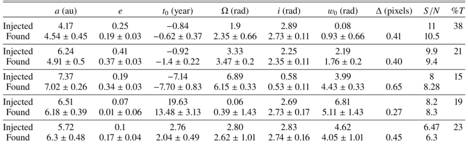
Appendix A: SHINE blind test
Table A.1. Orbital parameters of the injected and found planets (true positives) during the blind test described at Sect.3.
a (au) e t0(year) Ω(rad) i (rad) w0(rad) ∆(pixels) S/N %T
Injected 4.17 0.25 −0.84 1.9 2.89 0.08 11 38 Found 4.54 ± 0.45 0.19 ± 0.03 −0.62 ± 0.37 2.35 ± 0.66 2.73 ± 0.11 0.93 ± 0.66 0.41 10.5 Injected 6.24 0.41 −0.92 3.33 2.25 2.19 9.9 21 Found 4.91 ± 0.5 0.37 ± 0.03 −1.4 ± 0.22 3.47 ± 0.2 2.35 ± 0.11 1.76 ± 0.2 0.40 9.4 Injected 7.37 0.19 −7.14 6.89 0.58 3.99 8 15 Found 7.02 ± 0.26 0.34 ± 0.03 −7.70 ± 0.83 6.15 ± 0.33 0.53 ± 0.11 4.43 ± 0.33 0.65 8.28 Injected 6.51 0.07 19.63 0.06 2.69 6.81 8.2 19 Found 6.18 ± 0.39 0.01 ± 0.06 13.48 ± 3.13 0.39 ± 1.43 2.73 ± 0.17 5.11 ± 1.43 0.27 8.3 Injected 5.72 0.1 2.76 2.80 2.83 4.62 6.47 23 Found 6.3 ± 0.48 0.17 ± 0.04 2.04 ± 0.49 2.62 ± 1.01 2.74 ± 0.16 4.05 ± 1.01 0.45 6.3
Notes. ∆ (pixels) is the mean distance between the injected and found positions of the planet in the images. S/N is the S/N computed using the orbits of injection (S/N)totand the mean orbit found (S/N)KS. %T is the percentage of the covered orbit.
Table A.2. Distribution of the true north errors measured with SPHERE on the 47 Tucanae field (Maire et al. 2016).
Date (yr) True north (deg)
0. −1.813 0.1 −1.795 0.2 −1.758 0.3 −1.749 1.1 −1.761 1.2 −1.759 2.1 −1.739 2.2 −1.773 3.1 −1.8024 3.2 −1.804
Appendix B: SHINE IFS observations
Table B.1. Observations used in this paper.
Star name Obs. date JD NDIT × DIT Rot Seeing Prism Coro Algorithm Modes βPic 2015 Feb. 05 57058.02 316 × 8 88.36 0.89 Y–J APO1-ALC2 ASDI-PCA 50 βPic 2015 Sep. 30 57296.33 318 × 8 36.44 1.37 Y–J APO1-ALC2 ASDI-PCA 50 βPic 2015 Nov. 30 57356.23 880 × 4 39.72 1.85 Y–J APO1-ALC2 ASDI-PCA 50 βPic 2015 Dec. 26 57382.15 223 × 16 37.40 0.99 Y–J APO1-ALC2 ASDI-PCA 50 βPic 2016 Jan. 20 57407.10 160 × 16 29.54 1.07 Y–J APO1-ALC2 ASDI-PCA 50 βPic 2016 Apr. 15 57493.97 168 × 16 20.27 0.75 Y–J APO1-ALC2 ASDI-PCA 50 βPic 2016 Sep. 16 57647.36 348 × 16 38.77 0.78 Y–J APO1-ALC2 ASDI-PCA 50 βPic 2016 Oct. 14 57675.32 380 × 16 53.03 0.73 Y–J APO1-ALC2 ASDI-PCA 50 βPic 2016 Nov. 18 57710.25 564 × 4 44.20 0.78 Y–J APO1-ALC2 ASDI-PCA 50 βPic 2018 Sep. 17 58378.35 376 × 8 36.42 0.87 Y–J APO1-ALC2 ASDI-PCA 50 βPic 2018 Oct. 18 58409.31 432 × 8 54.40 0.78 Y–J APO1-ALC2 ASDI-PCA 50 HD 95086 2015 May 05 57147.04 47 × 64 17.42 0.72 Y–H APO1-ALC2 ASDI-PCA 50 HD 95086 2016 May 30 57538.97 61 × 64 25.63 0.48 Y–H APO1-ALC3 ASDI-PCA 50 HD 95086 2017 May 09 57882.96 99 × 64 36.55 0.94 Y–H APO1-ALC3 ASDI-PCA 50 HD 95086 2018 Jan. 06 58124.30 70 × 64 41.05 0.30 Y–H APO1-ALC3 ASDI-PCA 50 HD 95086 2018 Feb. 24 58173.19 64 × 96 33.59 0.32 Y–H APO1-ALC3 ASDI-PCA 50 HD 95086 2018 Mar. 28 58205.12 64 × 96 33.45 0.57 Y–H APO1-ALC2 ASDI-PCA 50 HD 95086 2019 Apr. 13 58586.07 63 × 96 33.84 1.05 Y–H APO1-ALC2 ASDI-PCA 50 HD 95086 2019 May 17 58620.99 64 × 96 33.29 0.84 Y–H APO1-ALC2 ASDI-PCA 50