Cyclic deformation of FCC crystals

Cyclic Deformation of FCC Crystals

by

Chuang-Chia LIN

B.S. in Mechanical Engineering,

National Taiwan University, 1990

Submitted to the Department of Mechanical Engineering

in partial fulfillment of the requirements for the degree of

Master of Science in Mechanical Engineering

at the

MASSACHUSETTS INSTITUTE OF TECHNOLOGY

January 1995

@ Massachusetts Institute of Technology 1995. All rights reserved.

Author .

---

-Author... ...

...

Department of Mechanical Engineering

January 5, 1995

Certified by ...

Lallit Anand

Professor of Mechanical Engineering

Thesis Supervisor

Accepted by ...

...

Ain Sonin

Chairman, Departmental Committee on Graduate Students

Eng.

Cyclic Deformation of FCC Crystals

by

Chuang-Chia LIN

B.S. in Mechanical Engineering, National Taiwan University, 1990

Submitted to the Department of Mechanical Engineering on January 5, 1995, in partial fulfillment of the

requirements for the degree of

Master of Science in Mechanical Engineering

Abstract

A combined experimental-computational program is conducted to develop a new crystal plasticity based constitutive model to predict the elastic-plastic deformation of fcc poly-crystals under multi-axial cyclic loading. Uni-axial strain and stress controlled cyclic tests along with multi-axial displacement controlled cyclic tests are performed on OFHC cop-per. As compared to the previous phenomenological cyclic plasticity models, this physically based combined isotropic-kinematic hardening crystal plasticity model demonstrates better agreement with experiments.

Thesis Supervisor: Lallit Anand

Acknowledgments

The first person I would like to thank is my advisor Professor Lallit Anand, a great thinker and a pioneer in the field of computational mechanics, for his guidance and support during the last two years. I also thank Professor Ali S. Argon for his excellent course which inspires my deep interest in materials behavior.

I also express my sincere appreciation to my girl friend, Liping Li, for all the support she gave me. Another special thanks goes to Dr. Christine Allan for the numerous discussions and helps she kindly initiated. Thanks to Don Fitzgerald for giving me so many friendly advises about machining and testing which I will always keep in mind. I also thank Dr. Jian Cao, Manish Kothari, Srihari Babrasupramanian, Dr. Hyungyil Lee, Dr. Fred Haubensak, Clearance Chui, Brian Gally, Surya Ganti, Alex Staroselsky, Hong Dai, Ming Zhou, John Zaroulis, Deborah Demania, and Lisa Tegeler for all their help.

Without many wonderful dinners with my best friends and former classmates, Kuo-Chang Chen and Kuo-Chun Wu, life in MIT would be further difficult. I am also grateful for Tian-Shiang Yang, Tong-Chien Tseng, Tomas Chao, Cynthia Chuang, Chen-An Chen and all other friends in ROCSA.

From dream to reality, I became a student of MIT. In the past seven hundred days, I have taken courses, made new friends, and tried to gradually melt myself into this new cultural environment. But the main subject which occupies my mind day by day, is the research work which leads to the superalloy model and this thesis. I would like to dedicate this thesis to the most important people in my life, my parents Chi-Fa Lin and Kung-Wei-Bao Lin, with my deepest gratitude and truest love.

Contents

1 Introduction

1.1 M otivation . . . .

1.2 Previous works . . . . 1.3 O bjective . . . . 2 Combined Isotropic-Kinematic Hardening Polycrystal Model

2.1 Specific Constitutive Equations ... 2.2 Time Integration Procedure ...

3 Verification of the Constitutive Model

3.1 Experimental Apparatus . . . . 3.2 Material Parameter Evaluation . . . . 3.3 Uniaxial Symmetric Strain Cycling . . . . 4 Predictions

4.1 Unsymmetric Axial Strain Cycling . . . 4.2 Unsymmetric Uniaxial Stress Cycling.. 4.3 Axial-Torsional Cycling ...

4.3.1 900 out-of-phase cycling ... 4.3.2 Butterfly strain cyclic test . . . .

4.4 Further predictions ...

4.4.1 Large strain torsion reversal test 4.4.2 Strain path change test ...

5 Closure 61 . . . . . 61 . . . . . 62 . . . . 63 . . . . . 63 . . . . . 65 . . . . 66 . . . . . 66 . . . . 67

List of Figures

1-1 Prediction of symmetric strain cyclic test with model of Kalindindi, Bronkhorst, and Anand, ea = 0.75% ... 21 1-2 Prediction of symmetric strain cyclic test with model of Kalindindi, Bronkhorst,

and Anand, ea = 1.5% ... 22 1-3 TEM pictures from Hasegawa and Yakou (1975). Dislocation density

de-creases at the initial stage of reversal (point C) . ... 23 1-4 Dislocation dissolution during reversal (Christodoulou et al. 1986) .... . 24 1-5 HVEM pictures shows diffusion of dislocation cell walls and tangles during

strain reversal. The left picture is taken before reversal, the right one is after. (Hasegawa and Yakou, 1980) ... 25 1-6 Stress strain response of reverse loading before and after annealing. The one

on the left compares reverse loading to forward loading after annealing, the curves on the right are all from reverse loading (Hasegawa and Yakou, 1980) 25 1-7 Two-stage strain path change test (Rauch and Schmitt, 1989) ... 26 1-8 Stress strain response for loading path change test. (Rauch and Schmitt, 1989) 27 1-9 Schematic drawing shows the typical Bauschinger effect. Compared to the

forward curve, there are: A. reduction of reverse yielding strength; B. smooth transition showing a strong hardening region; C. low hardening region; D. An offset in stress level (permanant softening ap). . ... 28 1-10 Unstable ratcheting of CS 1020 steel due to cyclic softening (Hassan and

Kyriakidas, 1994) ... ... 29 1-11 Four step unsymmetric strain cycling performed on SS 304 steel, the material

cyclic hardened in the first step, and showed slight relaxation in the last two steps (Hassan and Kyriakidas, 1994) ... ... 29

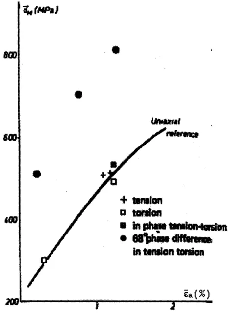
1-12 Tension, torsion, and combined-tension/torsion tests with different phase lags on 316 SS plotted on the saturation equivalent stress-equivalent strain am-plitude axis. It shows that the non-proportional cycling leads to higher sat-uration stress. (Cailletaud et al., 1984) . ...

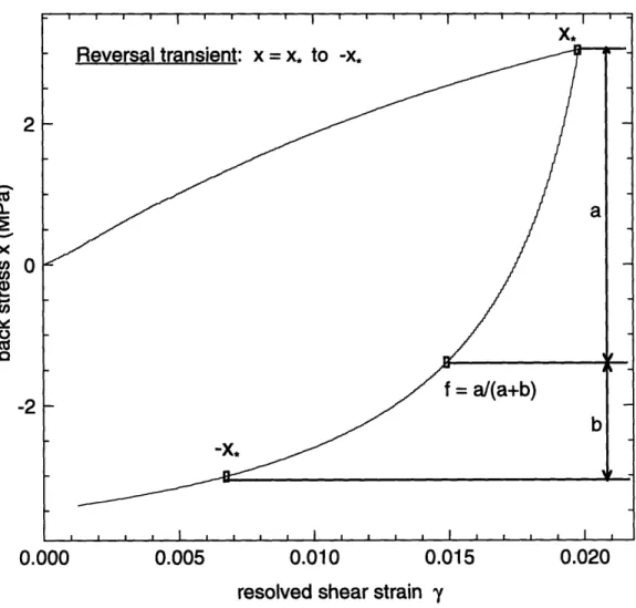
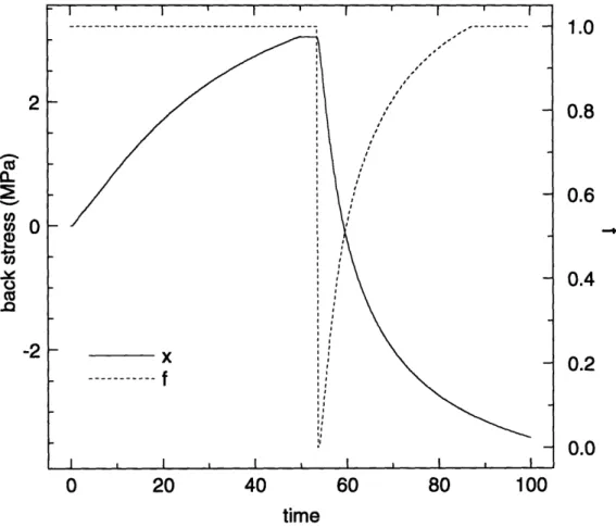
2-1 Definition of "reversal transient" and related parameters x,, and fraction f. 2-2 Evolution of f, and x versus time in a single reversal simulation. At the

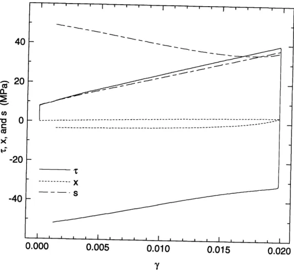
beginning of the reversal (time - 50), x,, is set to be equal to x and f to be zero. During the reversal, f increase to 1 while x keeps decreasing ... 2-3 Evolution for resolved shear stress (7), s and x versus resolved shear strain

in simulation ... 3-1 3-2 3-3 3-4 3-5

Instron biaxial testing frame...

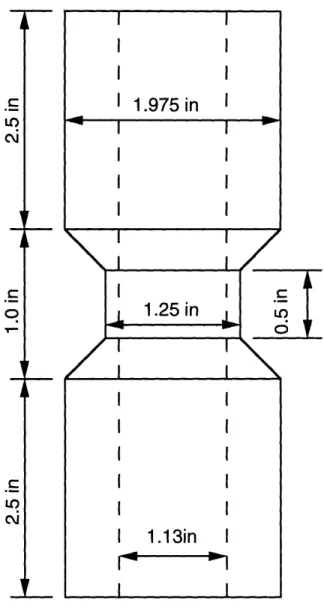
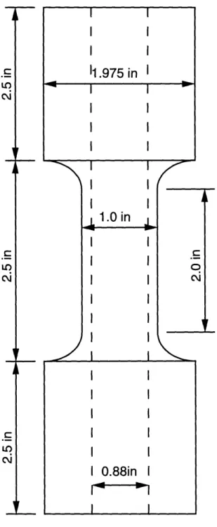
Tension-compression cyclic test sample. ... Axial-torsional cyclic test sample, short gage length . ... Axial-torsional cyclic test sample, long gage length . ...

Photo-micrograph of annealed OFHC copper taken perpendicular to the rod axis. (x1600) ... ... ...

3-6 Photo-micrograph of annealed OFHC copper taken (x 1600) . . . . . . . .. . . . . .. . . 3-7 Fit of x, and s for OFHC copper . . . . 3-8 Symmetric strain cycling test, Ca = 0.3% . . . . .

3-9 Symmetric strain cycling test, Ea = 0.5% . . . . .

3-10 Symmetric strain cycling test, Ca = 0.75% . . . . . 3-11 Symmetric strain cycling test, Ca = 1.5% . . . . .

3-12 Symmetric strain cycling test, Ca = 3% . . . . . .

. .. . . . .. . 53

parallel to the rod axis. . . . . . . .. . 54 . . . . . . . . 55 . . . . . . . . 56 . . . . . . . . . . . 57 . . . . . . . . . 58 . . . . . . . . . . 59 . . . . . . . . 60

4-1 Unsymmetric strain cycling test, c = 1% + 0.75% . ...

4-2 Schematic drawing shows the role of hardening in determining the ratcheting and relaxation behavior during cyclic deformation . ...

4-3 Ratcheting test...

4-4 Ratcheting test. Same data as in the last figure but the expermental result and the simulation are plotted separately. ...

4-5 900 out of phase biaxial cyclic test (-a = 1%, shearing first) ... . . 72

4-6 900 out of phase biaxial cyclic test (ia = 1%, tension first). . ... 73

4-7 900 out of phase biaxial cyclic test, Ea = 0.82%. . ... 74

4-8 Comparison of the saturation stress level between uniaxial and non-proportional 900 out-of-phase cyclic test with the same equivalent strain amplitude. (re-sults from simulation) ... . . ... 75

4-9 Strain path in a "butterfly" cyclic experiment. . ... . 76

4-10 Butterfly test ... .. ... .. .... ... 77

4-11 Large strain reversal torsion test, (Hu, Rauch, and Teodosiu, 1992). ... 78

4-12 Simulation of large strain reversal torsion test. . ... 79

List of Tables

Chapter 1

Introduction

1.1

Motivation

The development of mathematical models which describe and predict the deformation of metals is proceeding with increasing vigor. One of the existing features of the recent thrust toward plasticity modeling is its effort to bring together the separate disciplines of materials science and solid mechanics. This unification is motivated by recognition of the complexity and scope of the modeling activity. In order to provide an extrapolative and predictivitive capability, a strong physical basis is introduced into the modeling; and the multiaxial stress-strain relationship is expressed in an appropriate tensorial form. Multiaxial experimental work is conducted to determine the material parameters. Finally, numerical methods are developed to solve complex boundary values problems encountered in engineering design. Such interdisciplinary research allows development of constitutive models which comprehend and are founded on a strong physical basis, and also satisfy the requirement of a practical continuum theory.

A good example of the results of such an interdisciplinary approach is the polycrystal model developed by Anand, Kaladindi, and Bronkhorst (1991). They were the first to report a simulation and the corresponding comparison against experiments of the evolution of crystallographic texture in a non-homogeneous deformation processing operation, by using a Taylor-type polycrystal model at each integration point of a finite element mesh. A satisfactory agreement with experimental load-displacement curve and texture evolution was obtained. The advantage of using a crystal plasticity approach in modeling metal deformation is indicated by such success.

Indeed, a proper constitutive model is at the core of plasticity theory. However, a crystal plasticity model with only one internal resistance variable (Kalindindi, et al.,1991) has its limitations when applied to cyclic loading conditions. Their model is summarized below.

To simulate polycrystal deformations, we need to include enough grains with different orientations at each "material point". For a polycrystal materials, we assume that all grains have equal volume, and the local deformation gradient in each grain is homogeneous and identical to the macroscopic deformation gradient F at the continuum material point level. These assumptions leads to

N

Tr T(k) (1.1)

k=l

where T is the averaged stress, N is the total number of crystals at the material point, and

T(k) is the Cauchy stress in the kth crystal.

For each grain the constitutive equation for stress is taken as

T* = L [E*] (1.2)

with

E* = {F*F* - 1}, (1.3)

T* = F*- {(detF*) T} F*T, (1.4)

and £ a fourth order elasticity tensor. The strain and stress measure E* and T* are elastic work-conjugate strain and stress measures, with T the Cauchy stress tensor in each grain, and F* the local elastic deformation gradient defined by

F* = FF -1, (1.5)

where F and Fp

are the local deformation gradient and local plastic deformation gradient, respectively. In order to satisfy the condition of plastic incompressibility, det Fp _should

equal unity.

The plastic deformation gradient is in turn given by the flow rule

L

.asa,

a

S - ma

®

na

where m' and n' are time-independent orthonormal unit vectors which define the slip direction and the slip plane normal of the slip system a in a fixed reference configuration. The plastic shear rate on the slip system a is denoted by ý,a, and is defined in terms of the resolved shear stress 7-, and deformation resistance sa:

a

=

a

(7,

Sa)

)

.

The resolved shear stress Ta is obtained from balancing plastic stress power per unit

volume in the isoclinic relaxed configuration (e.g. Anand 1985)

0P - (C*T*)

-

Using the above equations, we defined a resolved shear stress Ta for the slip system a through the relation

(1.10) jip = I: T aY

a which yields

Ta (C*T*) - S' (1.11)

Since C* is approximately unity for small elastic stretches (which is true for metallic mate-rials), we have

Ta a T* .S . (1.12)

With sa representing the deformation resistance, the hardening rule is taken as

Shp _{haO = qa(P)h(-) no sum on 3}

(1.13)

where qap represents the latent hardening matrix. Following Asaro and Needlemen (1985),

(1.7)

for the 12 slip systems of FCC crystals, we have

A qA qA qA

qA A qA qA

(1.14)

[] qA qA A qA

qA qA qA A

here q is the ratio of latent hardening effect to the self hardening effect and A is a matrix fully populated by ones.

For the hV, motivated by Brown, Kim and Anand (1989), we take the following form

h

h

From the above equations, we see that the hardening rule for s" in a single slip defor-mation process with no latent hardening will be

sa = ho 1 - |- . (1.16) This equation for sa will lead to two response characteristics which are at variance with what is known about cyclic deformation:

1. Because s' is monotonically increasing, there would be no Bauschinger effect - no reduction of reverse yielding strength - during reversal.

2. Irrespective of the cyclic strain amplitude, the saturation level, ss, will be the same for all tests.

Fig. 1-1 and Fig. 1-2 show the prediction of two strain controlled tests (ea=0.75% and 1.5%) of polycrystal copper using the model of Kalindindi, et al with latent hardening. Although the initial monotonic stress-strain response is captured by the model very well, the prediction for the subsequent cyclic response does not match the experimental results. 'Therefore, the applicability of the previous model has to be restricted to monotonic defor-mations or to a small number of reversals. To overcome this weakness, it is required to modify the hardening rule and incorporate additional internal variables to better represent the slip system deformation resistance.

choice of appropriate internal variables and formulation of corresponding evolution equa-tions. The issue of how many variables a good model must contain can be viewed as a ques-tion of principle versus practicality. Incorporaques-tion of all possible micro-structural variables into a model seems impractical and hard to verify. Seeking direct quantitative representa-tion of micro-structure is also difficult. However, to provide an extrapolative capability it is required to incorporate internal variables derived from, or at least those that reflect, the internal structure. Also, these variables must be operationally defined to be measurable from physical experiments. Since a one internal variable model fails to represent cyclic deformation phenomena, in what follows we try two internal variables to characterize cyclic deformation. A common choice is the pair (s', za ) where s' is a deformation resistance and

:x' is a "back stress" variable. This choice has proved useful in several previous attempts at

cyclic crystal plasticity modelling applications (Stouffer 1992; Walker 1991; Teodosiu 1992). A flow rule generally accepted in these plasticity models is:

/0 I 1 if ITa

- xaI < sth,

a = (1.17)

o

Here Xz is the back stress for slip system a, and sth corresponds to a certain threshold resistance for all slip systems (for details see next chapter). The main difference between various models lies in the evolution equations for s' and za.

To make intelligent judgment and to extract physical laws from experimental observa-tions are the core characteristics of a successful model. In the light of this point, we begin with a brief review of previous research about the underlying mechanisms, and physical and macroscopic modeling for cyclic deformation. For a good review up to 1988, see White (1988).

1.2

Previous works

After Johann Bauschinger (1876-1886) reported the reduction of yield stress upon rever-sal of straining - _{the Bauschinger effect, the cause for such "anomalous" behavior had} remained mysterious for almost a century. The early suggestion around 1950's was that the Bauschinger effect is developed from plastic incompatibility between deforming grains. Acknowledging the fact that the Bauschinger effect is independent of grain size (Wolley,

1953), and exists even in single crystals (Marukawa and Sanpei 1971), we can conclude that the plastic incompatibility is not the only mechanism. Since for a single crystal of pure metal the main resource for shearing resistance is dislocation interaction with cells and tangles, the cause for the reduction of reverse yield should be due to the alteration of these micro-structural features.

Hasegawa, Yakou, and Karashima (1975) conducted experiments on polycrystal alu-minum and observed that dislocation cells, formed during prestraining, were dissolved at the initial stage of the reversed straining (Fig. 1-3). The overall dislocation density decreased by about 16% before increasing again. A similar result is also reported by Christodoulou, Woo, and MacEwen (1986) for polycrystal copper (Fig. 1-4). These structural changes are considered to be the origin of the Bauschinger effect in single phase metallic single crystals

in which cells or subgrains are formed during pre-straining.

This partial disintegration of cell walls and dislocation tangles was later studied by Hasegawa and Kocks (1979) and Hasegawa and Yakou (1980) to compare with the effects of annealing (thermo-recovery). It was found that although both thermo-recovery and stress reversal reduce reverse yielding, their physical background and subsequent macroscopic response are different. The thermo-recovery will tighten the cell walls, clean up the interior of cell, and eventually lead to annihilation of dislocations inside the cell walls. On the contrary, the reverse shearing will diffuse the cell wall (Fig. 1-5), make the micro structure similar to that of a less deformed material. Macroscopically, thermo-recovery reduces the reverse yielding stress more and in a uniform way but reversal shearing shows a transient, low hardening rate region (Fig. 1-6).

The comparison between the mechanisms for annealing and strain reversal reveals one piece of information: the dislocation structure could be divided into two categories: the one which is polarized and relatively unstable and the one which is isotropic and relatively stable. While annealing will eliminate both of them, the strain reversal would only annihilate the polarized one temporarily. This concept is quite useful for constructing cyclic constitutive models.

A reversal of strain in uniaxial cycling should be considered only a special case of a general loading process. With a lot of work focusing only on the Bauschinger effect in uniaxial cyclic loading, few people have noticed that the mechanism for the Bauschinger effect should also have an influence on any complex loading path change. Such a correlation

between the Bauschinger effect, load path change test, and micro-structure was recently investigated by Rauch and Schmitt (1989). They performed two-step tests on thin plate samples of mild steel. In the first step, they deformed the samples in tension; then, they performed simple shear tests on those predeformed sample with different angle (a) between the shear and the tensile directions (Fig. 1-7). They showed that when a equals 900 the yield stress is maximized and higher then forward flow stress, and when a equals 1350, a test similar to the typical Bauschinger test, the opposite is true (Fig. 1-8). The augmentation of yield stress when a equals 900 is explained by the observed formation of micro bands due to newly activated slip systems, and yield stress decrease (a = 135°) is, again, related to the dissolution of dislocation cell walls due to reversed shear stress on the same slip systems. What has been indicated by Rauch and Schmitt is the importance of the role of ,slip activity and the dissolution of dislocation cell structure upon reversal of slip on the same slip system.

The above experimental observations indicate that the deformation resistance, which could be expressed in terms of dislocation density, will not simply increase monotonously. In reality, the dislocation density will decrease during reversal, and this phenomenon is the cause for Bauschinger effect and related material behavior in a cyclic deformation process of pure single phase metallic crystal. Based on such an idea, White, Bronkhorst and Anand (1990) reported a phenomenological plasticity model with two internal variables, namely, deformation resistance and back stress. They also compared simulations of the model to uniaxial cyclic test data on five different materials - 1100-0 Aluminum, 316 stainless steel, and spherodized 1020, 1045 and 1095 plain carbon steels. The model was shown to capture the key features of these uniaxial cyclic behavior reasonably well.

A similar, but more complicated model was later on reported by Hu, Rauch and Teo-dosiu (1992). Based on the idea that the dislocation cell walls are polarized (Kocks, 1980), they separate the deformation resistance into three parts, (P, R, X). The part P is polarity dependent and is related to persistent dislocation structures, the part R is related to rear-rangement and formations, and the part X is related to less stable dislocation arrear-rangements. This model may be viewed as an extension of the model by White and Anand, but in a more complicated form. Their continuum plasticity model simulations match their large strain torsion tests data on AK-mild steel quite well.

ap-plication to single crystal superalloys. Stouffer and co-workers (1988, 1990, 1992) have pro-posed crystal plasticity models based on the idea of back stress. Walker and Jordan (1989, 1992) and Meric and Cailetlaud (1991) also present their combined isotropic-kinematic hardening model for superalloy PWA1480, and SNECMA AM1, respectively. Although there are complexities such as non-Schmid effect and temperature dependence in modeling superalloys, the small isotropic hardening of these highly strengthened two-phase materials usually allows simple isotropic hardening rules, such as non-hardening. Therefore, these models are not directly applicable to non-strengthened materials showing both hardening and softening in cyclic deformation.

Weng (1979, 1980, 1987) was one of the first to study kinematic hardening in cyclic loading in terms of crystal plasticity, and he approached this problem in a different way as compared to the other researchers. He consider the forward and reverse slip system as two different ones, and treated the Bauschinger effect as a latent hardening effect. Instead of using a single latent hardening ratio q (Equation 1.14), he express the latent hardening matrix q"a as:

qaP = qi + (1 - qi) cos BOb cos a + (q2 sin 0a + q3 sin0 a ) (1.18) where Oa0 is the angle between the slip direction and the ath and 3th systems, and 00P the angle between their slip plane normals. The three parameters ql, q2, and q3 are to be determined by latent hardening tests. With this interaction hardening matrix, he was able to reasonably match the latent hardening tests by Edward and Washburns (1954). His predictions of yield surface test of Philips and Tang (1972) were also good. Compared to the back stress models using simple latent hardening matrix (Eqn. 1.14), this approach may have some merit. However, such geometric based relationship can still not fully character-ize the nature of the hardening interactions. Besides, its application is more limited due its complicated slip interaction relations, and more tests are required to define the extra parameters such as ql, q2, and q3.

It is worth noting that there is another branch of cyclic plasticity models - the so-called two surface models - which have been developed by some workers in the last thirty years (e.g. Sierakowski, 1965; Morz, 1967, 1983; Dafalias and Popov, 1975, 1976). The general idea is to create one more (or multiple) bounding surfaces in addition to the yield surface in

stress space. The performance of such models depends on their specific equations specifying the translation and expansion of these bounding surfaces, and generally improves with the increasing number of surfaces or complexity of the specific equations. The latest model of this type is from Hassan and Kyriakidas (1994), which shows a good match with most of their uniaxial and biaxial ratcheting experiments on 304 and 1018 steels. However, they have to use different set of equations to reproduce the biaxial test than those they use for uniaxial tests. Also, their model is fairly complicated.

The general shortcomings of these two-surface phenomenological models lies in their lack of adaptability for extension to model anisotropic or inhomogenous materials, for instance, pre-textured polycrystals, two phase materials, or single crystals. It is also hard to reconcile these model for high temperature applications due to their rate-independent nature.

Recently, Khan and Su (1994) combined the latent hardening from Weng (1987), the forest dislocation relation from Jackson and Basinski (1967) and two-surface model similar to Dafalias and Popov (1976), and created a set of new constitutive relations for single crystals. They did a good job in matching the latent hardening test data of Edward et al. (1954) and Tang et al. (1972), but no prediction for multiple slip deformation is reported. Unlike the old two-surface models, some physical connections to dislocation densities and resolved shear stress are made to obtain equations for the bounding surfaces. This approach brings new insight to view the hardening mechanisms from constitutive modeling, but their lengthy formalism for more complicated slip activity seems to lack practicality.

1.3

Objective

With continuing efforts from researchers around the world, the picture of a general plasticity model has become more clear than ever before. Although there are no general guidelines for constructing such constitutive models, a crystal plasticity model with combined isotropic hardening and kinematic hardening, or in terms of internal variables, a deformation resis-tance and a backstress, seems to be a balanced choice between complexity and practicality for modeling of general deformations of metallic materials. Moreover, good multiaxial ex-perimental data have been lacking and most current phenomenological models show mod-erate predictability for multiaxial test results. Accordingly, an experimental-computational program is conducted to develop such a combined isotropic-kinematic hardening crystal

plasticity model. Appropriate specific constitutive equations are constructed based on crit-ical uniaxial/biaxial experiments with the objective of capturing the following important material behavior (White, Bronkhorst and Anand 1990):

1. Monotonic deformations:

* At low superposed pressures, initial yield and strain hardening are generally the same for uniaxial tensile or compressive deformation.

* If geometrical instabilities are suppressed, then strain hardening may continue to many hundred percent strain.

2. Uniaxial reversed and cyclic deformation:

* The Bauschinger effect: after deformation in one direction a reversal in the direction of deformation shows a reduced stress magnitude when yielding occurs again. There is usually a smooth transition from elastic to elastic-plastic behavior upon development of plastic flow in the reverse direction. As the tangent modulus gradually decreases and achieves the value it had prior to unloading, there may be a "permanent softening" where the flow stress magnitude is less than it would have been in unidirectional loading at the same accumulated strain. (Fig. 1-9)

* Under symmetric cycles of strain (or stress) metals in a annealed state will harden cyclically and tend to stable limit cycle (Fig. 1-1 and 1-2), while those in a cold worked condition will soften to a stable cycle.

* Unsymmetric cycles of stress in the plastic range will cause progressive "creep" or

"ratcheting" in the direction of the mean stress. Depending on the material, the strain increment might stabilize during ratcheting, or becomes unstable as in Fig. 1-10.

* Unsymmetric cycles of strain for cold worked metals in the plastic range will cause

progressive relaxation to zero of the mean stress in the cycle. For annealed metals, the material will harden cyclically to a stable loop as in the symmetric strain cycling case. Softening might appear as the annealed material is continued to be cycled to large number of cycles, or in a multi-step unsymmetric strain cycling test (Fig. 1-11). 3. Small strain multiaxial cyclic deformation:

* Proportional cycles of combined tension-torsion for a given equivalent strain amplitude

gives rise to an "equivalent" cyclic stress-strain response which is the same as that obtained in uniaxial strain cycling for the same strain amplitude.

* Non-proportional tension-torsion cycling exhibits higher hardening and higher

satu-ration stress levels for cycling to the same maximum equivalent strain amplitude as compared to proportional cycling (Fig. 1-12). The combined out-of-phase tension-torsion test with a phase difference of 90 degrees causes the largest cyclic hardening of all possible paths with the same strain range.

In the following chapters, we present the results of the current study with the objective of capturing the above criteria. Attension is first focused on the constitutive equations, which, combined with time-integration schemes, will be introduced in the next chapter.

OFHC copper cyclic test (RT)

200

100

0

-100

-200

x10-3

true strain

Figure 1-1: Prediction of symmetric strain cyclic test with model of Kalindindi, Bronkhorst,

and Anand, Ca = 0.75%. i I i i I I I I I

simulation

-

-

-

-experiment

-

-

- - - -

-

-cr---OFHC copper cyclic test (RT)

- -- I-u-a-i I I - - - - - '

--

simulation

-0.01

0.00

0.01

true strain

Figure 1-2: Prediction of symmetric strain cyclic test with model of Kalindindi, Bronkhorst, and Anand, Ca = 1.5%.

200

O

-200

-i

a

Figure 1-3: TEM pictures from Hasegawa and Yakou (1975). Dislocation density decreases at the initial stage of reversal (point C)

Stress 130 60 -10 -80 -0.03 -0.01 0.01

True plastic strain

Figure 1-4: Dislocation dissolution during reversal (Christodoulou et al. 1986)

!D

B _Annealed HCCu

---

Figure 1-5: HVEM pictures shows diffusion of dislocation cell walls and tangles during strain reversal. The left picture is taken before reversal, the right one is after. (Hasegawa and Yakou, 1980)

I (%)

_S(

_W1

Figure 1-6: Stress strain response of reverse loading before and after annealing. The one on the left compares reverse loading to forward loading after annealing, the curves on the right are all from reverse loading (Hasegawa and Yakou, 1980)

STAGE 1. TENSION ON LARGE PLATE SAMPLE a

A/

STAGE 2. SHEAR ON SMALL CUT SQUARE SAMPLE

'

Figure 1-7: Two-stage strain path change test (Rauch and Schmitt, 1989)

I

I

I

/

*Do in*o so 0 'lewgr •rvw• -mper mwrvmm n I, # .10e1&e oure u * ***

rY

!~

Figure 1-8: Stress strain response for loading path change test. (Rauch and Schmitt, 1989)

_ _~_~~_

& ... • •

Irl

.

C

Figure 1-9: Schematic drawing shows the typical Bauschinger effect. Compared to the forward curve, there are: A. reduction of reverse yielding strength; B. smooth transition showing a strong hardening region; C. low hardening region; D. An offset in stress level (permanant softening op).

(ksi)

-5

Figure 1-10: Unstable ratcheting of CS 1020 steel due to cyclic softening (Hassan and Kyriakidas, 1994)

Ia

Figure 1-11: Four step unsymmetric strain cycling performed on SS 304 steel, the material cyclic hardened in the first step, and showed slight relaxation in the last two steps (Hassan and Kyriakidas, 1994)

SW

SW

4WI

SAN

.M%

WaWiW

I

in

toll?$=lan

UU2lrriam

fl

Figure 1-12: Tension, torsion, and combined-tension/torsion tests with different phase lags on 316 SS plotted on the saturation equivalent stress-equivalent strain amplitude axis. It shows that the non-proportional cycling leads to higher saturation stress. (Cailletaud et al., 1984)

Chapter 2

Combined Isotropic-Kinematic

Hardening Polycrystal Model

The present work extends the polycrystal visco-plasticity model of Anand and co-worker (Bronkhorst et al., 1991 and Kalindindi et al.,1991). Basically, in addition to the slip resis-tance s' of Anand, et al., we introduce another internal variable, a "back stress" parameter xa on each slip system, and corresponding evolution equations to represent the essence of anisotropic hardening during cyclic deformation process. The slip resistance s" is related to the forest dislocation density in a physical sense, and the directional resisting strength developed during shearing is represented by the back stress xa. New equations for ya and

the evolution equations for s' and x" are formulated. These equations are introduced in the following sections.

2.1

Specific Constitutive Equations

For the cubic crystals considered in the current research, the description of the elasticity tensor £ requires three stiffness parameters, C1 1, C12, and C4 4, which are defined as:

C11 = (e ® e' ).[e' ®e] (2.1)

C12 = (e ®e) .£[e' ®e] (2.2)

C44 = (e' ® e') £[2sym(ef( e')] (2.3)

There are several features of a typical uniaxial cyclic stress strain relationship that we should consider while constructing the model. Initially, the reverse proportional limit is lower than the forward flow stress. Secondly, an initial high hardening rate region accom-panied by a relatively long region of low hardening are usually observed, showing a plateau on the curve. Finally, as the reverse hardening rate approaches the forward hardening rate there is an offset in the stress magnitude at equal accumulated strain level. Such an offset is often referred to as "permanent softening" in the literature.

To match these features, the specific constitutive functions for the plastic shearing rate

ja is taken as

0 if IrT' -a < Sth

0

=

-XIs

_(2.4)

0 ( s thm sign(Ta -x a) if

IT

where j0o and m are material parameters representing a reference shearing rate and shear rate sensitivity. The parameter sth represents a threshold value for the effective stress

(7" - x") below which no shearing occurs in slip system a. For pure metals, sth is in the order of 0.1 Mpa. The parameter so is the shearing resistance, and x' is the back stress.

Motivated by White, Bronkhorst and Anand (1990), the slip resistance s' is taken to evolve as

h= a

hc'P

[-ha

(2.5)

where

ha- = qa(P)h#

)

_{(no sum on}

f),

_(2.6)

and

h =

-

(2.7)

The first part of (2.5) is essentially the same as the hardening rule from the crystal plasticity model by Anand and co-workers. Here r, s,, and a are constants, and s, denotes the saturation value for s.

The second part in ( 2.5) represents the softening effect in cyclic loading. The h' stands for the rate of softening on slip system a due to a reversal of shearing on that system. Previous experimental results in the literature indicate that the softening effect is active only during the "reversal transient" which is (approximately) limited to the time that it

takes for the back stress to change sign and achieve the same magnitude it had prior to the reversal. In order to properly define the softening modulus hl, we generalize such an idea and operationally define the "reversal transient" and related parameters in our model as follows:

" During a cyclic loading process, a reversal transient for a slip system commences when ýa or the effective stress (7- -

x')

t,

reversal transient commences, and let

x, = X (tn) (2.8)

denote the value of xa at the beginning of the reversal event.

* A reversal transient ends when the back stress reaches the same magnitude but op-posite sign as when the transient started. That is, a reversal transient ends when

za(7)

= --

x,

7

>

t,

(2.9)

* Let fa denote the fraction of a reversal event the slip system has experienced. Refer-ring to Fig. 2-1 and 2-2, fa is defined as

0 when (r' - xa) changes sign,

f

We define the softening rate h' based on the following ideas. We assume that h' * Vanishes as fa approaches unity.

* Is proportional to x14 .

Accordingly, we assume that

hc = ( (1 - fa) (14xl) (2.11) Here ( is taken as a constant.

In (2.11), we assume that the softening rate h₂ is proportional to the maximum opposing stress ,* I. A additional inverse dependence of (Ix, + sth) is found necessary to correctly

model the small strain cyclic response (Ea < 0.5%). Numerical experiments showed that when the cyclic strain amplitude is less than 0.5%, the softening effect needs to be en-hanced to more accurately reproduce the experimental data. We assume a simple inverse relationship of Ijxal to represent this observation. To prevent the singularity of this term for situations when

lxc1l

h

•=(1

- fa)

(

xa

l

This relative strong softening effect in small strain cycling may be qualitatively explained by the following arguments. In small strain cyclic deformations, planar vein structures consisting of edge dislocation bundles are observed. The existence of such planar vein structures have been verified for single crystals (e.g. Basinski, Basinski, and Howie 1969), and also individual grain of polycrystals (e.g. Liu, You, and Bassin 1994). Based on purely geometrical considerations, it seems reasonable to argue that a planar dislocation structure is easier to dissolve on reversed deformation as compared to a three dimensional cell network formed during large strain cycling. Since these planar structures mainly appear during small strain cycling, we find stronger softening during small strain cycling. To model such effect, we take a first order approach and assume h2 to be simply inversely dependent on jIx I + Sth.

A good match between the simulation results and experimental data justifies the utility of including such a term (Chap. 3).

Next, for the evolution for the back stress we assume

3 (1 - -sign (-ýa)) -ya

(2.13)

X8

where h' is the rate of hardening for the back stress.

As indicated in Chap.1, it has been experimentally observed that at the beginning of stress reversal, the dislocation cell walls will disintegrate (Hasegawa and Yakou, 1975) and reduce the slip resistance(s). In the mean time, the back stress also changes sign. Therefore the rate of softening for s _{and the rate of change of back stress are coupled. In this model,}

form for h3

h" = € + Xha, (2.14) where

4

The set of equations (2.4) through (2.14) is aimed at representing the major features of the flow stress evolution in a typical cyclic test. Using representative values of material parmeters, Fig. 2-3 schematically shows the evolution of 7r, xa , and so for one slip system of a single crystal undergoing single reversal. Before the reversal, the resolved shear stress reaches 40 MPa, but the reverse yield strength drops to 36 MPa. The difference between the forward the reverse flow stress is approximately equal to two times the back stress at reversal. As back stress changes sign and hardens in the other direction after reversal, there is a corresponding low hardening region for the stress and the s also softens reasonably. These three effect are coupled together through the constitutive equations introduced above. To further examine the contribution from each terms from the constitutive equation, we invert (2.4), and we will get

Ira-XI

-

Sth

=

(2.15)

Let 7• > xa before reversal and assume sth to be small and negligible, then

7. (00 a + a ." (2.16)

After reversal, the relationship becomes

- T·o S -- X . (2.17)

Taking absolute value of the above two equations, it is not hard to see that whenever -7 changes sign, the magnitude of the reverse yield stress will be reduced by two times the value of current xa. Accordingly, from Eqn. 2.13, we see that ia will change sign at reversal straining and its magnitude will be relatively large at the beginning before it goes down, showing a high initial hardening rate for the flow stress.

At the same time, the hardening rate sa reduces during the reversal transient due to the increasing contribution from h2, and we get a plateau on the stress strain curve

(Fig. 2-3). Eventually, as x' reaches the same magnitude as before reversal (the end the reversal transient), the s' has not hardened very much due to the softening effect during the reversal transient. Therefore, we would observe an offset between the forward and reverse stress levels -the permanent softening - on an accumulated strain-stress diagram.

Having examined the interaction between the constitutive equations for single slip, let us summarize the complete model for a single crystal as follows:

1. Constitutive Equation for Stress:

T* = L [E*]

{

F*

=

aS

Xal

m

sign

Ir

>

T7a T*

-S0

(2.24)

(2.25)

3. Evolution Equations for sa:

(2.26)

( no sum on # )

h?' = qQaph (2.27)

0

A

qA qA

qA

qA qA

A

qA

qA qA qA

A

(ii

+

(2.30)

0 when (ra - xa) changes sign

f-

1

1-

-

=

(2.31)

1 when xw = -x

4. Evolution Equations for xa:

a-= ha (1 sign ('a)) < (2.32)

ha = € + Xh2 (2.33)

2.2

Time Integration Procedure

Let t denote the current time, and r = _{t + At the time at the end of an increment. Then,}

proceeding in a fasion similar to the time integration procedure for a polycrystal plastic-ity model without back stress (Kalidindi, 1992), we start from solving a set of nonlinear, simultaneous algebraic equations in T*(r) ,sa(7), and x'a(7). The equation for T*(7) and

sa(r) is quite similar to the previous work:

T*

(r)

s

C

where

T*tr" £[( A - 1}

Ca

a

[(

Ba]

A Fp - T (t) FT () F (7) FP -' (t) Ba - AS +SSA

To obtain the equation for xa(r), from (2.32), we recall that

(

1

h" = 0 + XC (1 - f ") jx.

Xl+

h

(2.40)

and note that since h' is a function of xz only, the rate equation (2.32) can be expressed as a function of x' as follows:

-

-sign

Xs

(ýa))

-ia

(2.41)

The equation can be analytically integrated from time t to time 7 assuming that the ya

does not change sign during the interval (t - 7):

("(T) _dx

Ix(t)

(2.42)

= dWy~

Jr" (t

Carrying out the integration and substitute in the value of xz(t), we get

Xz()

=

_(be

ae

- 1

-

d)

a =

+

~xIxx I

I

_-

_,x

.a

₃

a

e = -dxa(t) exp((b - a d)Aya(a (T*(r)), sa(7),xa(T))) (2.47)

a-b- xa(t)

Equations (2.34), (2.36) and (2.43) are solved using a two level iteration procedure. The subscripts n and k, through this section, refer to the number of first level iterations, and second level iterations, respectively. The subscript p for xp (7) refers to the xa (7) obtained at pth trial of the whole iteration process.

In the first level of iteration, Eqn. 2.34 is solved for T*(T) using Newton-type algorithm while keeping the estimates of s" (r) and xz (7) fixed. The Newton algorithm for T*(T) is

Tn+1 (r) = T* (t) - Jn-' [G,] (2.48) where

Tn

C)()

a

a

As the iteration of the stress converges, we start the pth trial of the second level iteration by updating the value of xp (T) using (2.43) with e in (2.47) estimated by Tt 1(7r), s (7)

and xP_l1(7r). After we obtain xx(T7) and accordingly, h(7T), we are able to calculate an

average value for h" during t to 7

M

h2(t) + h• (7)

h 2 (2.51)

Using this averaged h', we start the second iteration by iterating the sa (7) as:

S

+

1(7)

s=

a(t)

+

((T))

Ih

[A

7

(

(T

1

(7))

, s (),

1

(7))

(2.52)

-h (xa(t), xc(7-)) 1 A- (Ta' (T+ 1(T)) , c' (r) , (T))

In our calculation, the values of T* (7) and sa (T) are accepted if change in the absolute values are less than 10-3so for T* (T) and 10-4so for sa (7). Otherwise, this new estimates of

sa (T) and xa (T) are used to restart the iteration. Since we use an exact analytic integration to calculate xa (T) from t to T, it only need to be calculated once at the beginning of each second level iteration and its convergence is implied by the convergence of T*(7) and sa(-).

The remaining task for time-integration scheme is essentially the same as the polycrystal model by Kalidindi, Bronkhorst and Anand (1991).

In the next chapter, we verify our model by comparing a set of experimental data to simulation results based on experimentally obtained parameters. We will show that the validity of the model is supported by a good match between the simulation and experimental results.

-2

0.000

0.005

0.010

0.015

0.020

resolved shear strain

y

2

0

S0

-2

-2

II,

0

20

40

60

80

100

time

Figure 2-2: Evolution of f, and x versus time in a single reversal simulation. At the

beginning of the reversal (time ; 50), x, is set to be equal to x and f to be zero. During

the reversal,

f

increase to 1 while x keeps decreasing.

1.0

0.8

0.6

0.4

0.2

0.0

40

.- 20

I--20

-40

u.uuU

0.005

0.010

0.015

0.020

Figure 2-3: Evolution for resolved shear stress

(T),

_{s and x versus resolved shear strain in}

Chapter 3

Verification of the Constitutive

Model

3.1

Experimental Apparatus

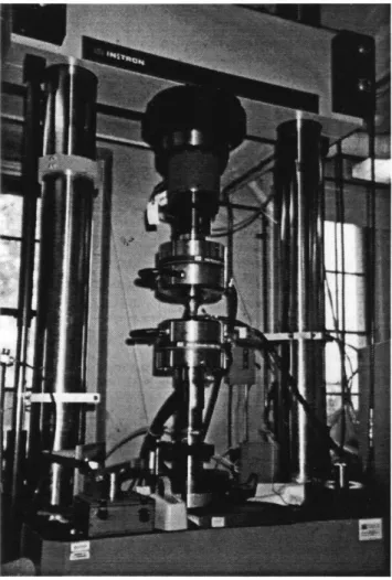
The experiments were conducted on a stiff servo-hydraulic testing system (Fig. 3-1). The testing system features a high stiffness biaxial test frame equipped with MTS series 646 hydraulic collet grips, and the load capacity is 50,000 lbs (222 kN) / 20,000 inch-lbs (2260 N-m). The machine is controlled on both channels with an analog controller. Acquisition of data is performed with the software package LabTech Notebook through a Keithley Series 500 hardware interface installed on an Intel 486/50 personal computer. Prior to the tests, the load train is carefully aligned by adjusting four alignment screws on the top of the load train to make sure that the misalignment is less than 0.0005" circumferentially.

High conductivity oxygen free copper is chosen as the candidate material for all testing. Round tension-compression and tension-torsion specimens are machined from as-received 0.5" and 2" diameter rods. The dimensions of the uniaxial test sample and axial-torsional sample are shown in Fig. 3-2 and Figs. 3-3, 3-4, respectively. Prior to the tests, all samples were annealed in an Argon-filled furnace, to remove any residual stress or pre-textures. The samples were heated up to 8000C in two hours, soaked for one hour and then furnace cooled to room temperature in nine hours. After annealing, photo-micrographs of the polished-etched sample were taken ( Figs. 3-5, 3-6). The grains are equiaxed and their average size is about 60 pm. The annealed material shows a relatively low yield strength of 25 MPa.

The uniaxial tension/compression cyclic test were performed under strain and load con-trol mode to precisely characterize the strain in the gage section. For these tests, the strain data are collected through an extensometer with maximum range of

±0.1

Lacking a biaxial extensometer, the biaxial cyclic test were performed under position control. However, a strain gage rosette was carefully aligned and glued on the surface of the gage section of the specimen to provide a measurement of the cyclic strain in the gage section. During the test, displacement readings from LVDT and RVDT are collected together with the readings from the strain gages. These two data are compared to check the accuracy of LVDT/RVDT readings in providing accurate measures of gage section strains. Noting that the relative importance of the shoulder sections depends on their length, as compared to gage length, it is found that the deformation of the shoulder sections plays a less important role for the tests performed on the long gage length torsional samples. The strain amplitude is almost uniform through the test. For the short gage section samples, the deformation in the shoulder section is relatively larger.

3.2

Material Parameter Evaluation

In order to perform numerical simulations using the present model, we need to estimate the material parameters. The parameters in the present model include elastic modulus C11, C12, C44, rate sensitivity m, plastic resistance parameters so, s,, Xz, Sth, and hardening

parameters a, l7, ýj , X, and q. In this section, a methodology for determining the material parameters is given and applied to the material under consideration.

The experiments that were required to determine the parameters consisted of the uni-axial monotonic test and the uniuni-axial cyclic tests, and the steps used to determine the material parameters are as follows:

1. Obtain C11, C12, and C44 from handbooks.

Elastic moduli C₁₁,

C

copper are available in handbooks (e.g. Simmons and Wang, 1971). 2. Determine m and q.

The value of rate sensitivity m for OFHC copper is obtained by fitting a uniaxial strain rate jump test performed by Bronkhorst (1991) with ~o set to be equal to macroscopic strain rate. Characterization of latent hardening is perhaps the most difficult part of the

constitutive model. Here we simply take the latent hardening factor q as 1.4. 3. Determine 0 and x, from uniaxial single reverse test.

Several symmetric strain cycling tests with different strain amplitudes were performed in order to determine the back stress versus strain curve, by utilizing the first reversal data. We define the level of back stress at each strain amplitude to be half of the difference of corresponding forward flow stress and reverse 0.2% offset yield stress. For polycrystal mate-rials, the averaged resolved shear stress is about one-third of the macroscopic tensile stress. Using this relation, we can approximate the resolved-shear-stress/strain curve. On the other hand, because during a monotonic deformation the term contains X in the expression for

h₃ is zero, h3 equals ¢ and we can integrate Eqn. 2.32

dx 7

L

dx

d7

(3.1)

and get the back stress- strain relationship

S-

=n

(3.2)

The initial guess of x, and 0 is obtained by nonlinear fitting such equation to the back stress-strain (x - -y) curve. These values are then checked and fine-tuned using a finite element

simulation of a monotonic test. Fig. 3-7 shows the results from fitting the experiment data of OFHC copper.

4. Determine a, 7, so, ss, and q from uniaxial monotonic test.

After the back stress-strain curve are determined, we can exclude its contribution from the total resistance (flow stress) and get the isotropic resistance-strain data. Since h2

is zero during a monotonic test, the deformation resistance-strain relation (2.5) is again integratable without considering latent hardening effect.

f

ds

a

Idy

then

l(a - i) - = _(3.4) Therefore, a first guess of so, s, ,a and t7 _{could be obtained using similar procedures as for}

x, and 0 from nonlinear curve fitting (3.4) to the resistance-strain data . From experience

it is found that we need to reduce 7r by about 5 times and adjust a a little bit after including the latent hardening relationship for s. After a few trials, a proper set of a, i7, so, and s,

will be obtained to give a reasonable fit the monotonic stress strain response (Fig. 3-7). 5. Determine X and ( from fitting the uniaxial cyclic tests.

After all other parameters are determined, ( and X is obtained by trial and error to get a best fit of at least two stress-strain curve from the uniaxial cyclic tests data. The general rule for adjusting these two parameters is: increase X to increase the initial slope of each reversal and saturation stress level; increase ( to increase the permanent softening and reduce the saturation stress level. Since there is a competing effect between ý and X, it requires a few trials to get these two parameters.

The complete set of parameters for Copper obtained is listed in Table 3.1 below. Where

a, m, and q are dimensionless and the rest have dimension of MPa.

C

₁

C

C

R

X

150.E+3 110.E+3 75.E+3 325.0 138.0 448.0 1.5625

so sS 2x a m q

8.0 133.0 5.0 2.1 0.012 1.4

Table 3.1: Material parameters for annealed OFHC copper

3.3

Uniaxial Symmetric Strain Cycling

To verify our cyclic crystal plasticity model, we check its performance by matching cyclic tests with equal positive and negative cycling strain range-the symmetric strain cycling. The model should be able to capture the whole deformation process for each strain range, up to the saturation level. These tests are also the primary tests for determining the set of material parameters, as indicated in the previous section.

Five tests, with strain range of 0.3% to 3%, are performed and the tests data and simulations are shown in Fig. 3-8 to 3-12. The model are able to closely match the stress-strain response up to saturation. There is some discrepancy in the vicinity of each reversal; the simulation shows a little sharper turn in this regime.