HAL Id: hal-00564360
https://hal.archives-ouvertes.fr/hal-00564360
Submitted on 8 Feb 2011
HAL is a multi-disciplinary open access
archive for the deposit and dissemination of
sci-entific research documents, whether they are
pub-lished or not. The documents may come from
teaching and research institutions in France or
abroad, or from public or private research centers.
L’archive ouverte pluridisciplinaire HAL, est
destinée au dépôt et à la diffusion de documents
scientifiques de niveau recherche, publiés ou non,
émanant des établissements d’enseignement et de
recherche français ou étrangers, des laboratoires
publics ou privés.
numerical simulations of spilling breaking waves
Pierre Lubin, Stéphane Glockner, Olivier Kimmoun, Hubert Branger
To cite this version:
Pierre Lubin, Stéphane Glockner, Olivier Kimmoun, Hubert Branger. numerical simulations of spilling
breaking waves. Conference on coastal engineering, Jun 2010, Shangai, China. pp.1-9. �hal-00564360�
1
Pierre Lubin1, Stéphane Glockner1, Olivier Kimmoun2 and Hubert Branger3
Numerical simulation of spilling breaking waves is still a very challenging aim to achieve since small interface deformations, air entrainment and vorticity generation are involved during the early stage of the breaking of the wave. High mesh grid resolutions and appropriate numerical methods are required to capture accurately the length scales of the complex mechanisms responsible for the start of the breaking (small plunging jet, white foam, etc.). Numerical works usually showed better agreements when simulating plunging breaking waves than the spilling case compared with available experimental data. Kimmoun and Branger (2007) recently experimented surf-zone breaking waves. Detailed pictures showed a short spilling event occurred at the crest of the waves, before degenerating into strong plunging breaker. This work is devoted to the qualitative comparison of our numerical results with the experimental observations, as we will focus on capturing and describing the spilling phase experimented.
Keywords: breaking waves; Navier-Stokes; numerical simulations; Large Eddy Simulation
INTRODUCTION
Simulating the air entrainment phenomenon generated by breaking waves remains a major challenge for modern CFD tools (Sakaï et al. 1986, Christensen et al. 2002, Christensen 2006, Watanabe 2005, Lubin et al. 2006b). Numerous problems motivated by fundamental research and applications, from environmental and coastal engineering sciences, require accurate description of wave breaking. Highly complex hydrodynamic features are usually encountered in the surf zone: transition from irrotational flow motion to high frequency turbulence, interacting with large- and small-scale interface deformations, from overturning and breaking of the waves to complex fractioning and coalescence of bubbles and droplets (Miller 1976, Bonmarin 1989). A broad range of relevant length and time scales is thus involved in this multiphase turbulent flow, making it extremely complicated to investigate experimentally and numerically (Battjes 1988).
Kimmoun and Branger (2007) recently experimented surf-zone breaking waves. Particle Image Velocimetry (PIV) experimental techniques were improved to be able to calculate velocities and void fractions in the aerated regions. Detailed pictures showed a short spilling event occurred at the crest of the waves, before degenerating into strong plunging breaker. Numerical works usually showed better agreements when simulating plunging breaking waves than the spilling case compared with available experimental data. Fine mesh grid resolutions and appropriate numerical methods are required to describe accurately the length scales of the interface deformations experimentally measured (plunging jet, white foam, etc.).
The aim of this paper is to simulate this unsteady two-phase wave breaking motion using a LES method to gain a further understanding of the complicated features of the flow. We aim at describing accurately the free-surface behavior, as we will focus on capturing and describing the spilling phase experimented by Kimmoun and Branger (2007).
MODEL AND NUMERICAL METHODS
We solve the Navier-Stokes equations in air and water, coupled with a subgrid scale turbulence model. The numerical tool is well suited to deal with strong interface deformations occurring during wave breaking, for example, and with turbulence modeling in the presence of a free-surface in a more general way.
Governing equations
An incompressible multiphase phase flow between non-miscible fluids can be described by the Navier-Stokes equations in their multiphase form. The governing equations for the Large Eddy Simulation (LES) of an incompressible fluid flow are classically derived by applying a convolution filter to the unsteady Navier-Stokes equations. In the single fluid formulation of the problem, a phase function C, or ”color” function, is used to locate the different fluids standing C = 0 in the outer medium, C = 1 in the considered medium. The interface between two media is repaired by the discontinuity of C
1 TREFLE UMR CNRS 8508, Université de Bordeaux, IPB, 16 avenue Pey-Berland, Pessac, France 2 CMRT, Ecole Centrale de Marseille, 38 rue Joliot Curie, Marseille, France
3
COASTAL ENGINEERING 2010 2
between 0 and 1. In practice, C = 0.5 is used to characterize this surface. The resulting set of equations reads (Eqs. 1-4):
0
.
u
(1)
( t )
T p t K
u u u g u u F u (2).
0
C
C
t
u
(3)with velocity u and pressure p, assuming g as the gravity vector, ρ as the density, µ as the viscosity, µT
as the turbulent viscosity, t as the time and F as the superficial tension volume force.
The magnitudes of the physical characteristics of the fluids are defined according to C in a continuous manner as:
1 0 1 0 (1 ) (1 ) C C C C
(4)where ρ0, ρ1, µ0 and µ1 are the densities and viscosities of fluid 0 and 1 respectively.
To deal with solid obstacles within the numerical domain, it is possible to use multi-grid domains, but it is often much simpler to implement the Brinkman theory, then considering the numerical domain as a unique porous medium. The permeability coefficient K defines the capability of a porous medium to let pass the fluids more or less freely through it. A real porous medium is modeled with intermediate values of K. If this permeability coefficient is large (K + ∞), the medium is equivalent to a fluid. If it
is zero, we can model an impermeable solid. It is then possible to model moving rigid boundaries or complex geometries. To take this coefficient K into account in our system of equations, we thus add an extra term, called Darcy term, (µ / K) u.
The turbulent viscosity μT is calculated with the Mixed Scale model (Sagaut 1998), which has
proved its accuracy for geophysical flows (Lubin 2004; Helluy et al. 2005; Lubin et al. 2006b, Lubin et al. 2010a-2010b). Based on the review of Lubin and Caltagirone (2010), we find that the most widely used subgrid scale model is the Smagorinsky model. However, it has been proved to be much too dissipative (Sagaut 1998). In spite of its negative aspects, its simplicity is still widely appreciated.
We use the procedure of regular and irregular wave generation developed by Lin and Liu (1999b). The method consists in introducing an internal mass source function in the continuity equation (Eq. 1) for a chosen group of cells defining the source region. The method have been extensively verified and validated compared with analytical profiles to ensure accurate wave generation.
Model (Eqs. 1 to 4) describes the entire hydrodynamics and geometrical processes involved in the motion of multiphase media.
Numerical methods
The time discretization is implicit and the equations are discretized on a staggered grid thanks to the finite volume method. A dual grid, or underlying grid (Rudman 1998), is used to gain an improved accuracy for the interface description, the mesh grid size being divided by two in each direction for the interface tracking. This technique also allows to avoid the interpolations of the physical characteristics on the staggered grids, since the color function is defined on each point where viscosities and densities are needed.
The interface tracking is achieved by a Volume Of Fluid method (VOF), which is able to handle interface reconnections without interface reconstruction. The explicit Total Variation Decreasing (TVD) Lax-Wendroff (LW) scheme of LeVeque (1992) is used to solve directly the interface evolutions without the reconstruction of C (Eq. 3). Lin and Liu (1999a) gave a complete overview and discussion of the different numerical techniques that have been used for the interface tracking in numerical simulations of breaking waves.
The numerical code has already been extensively verified and validated through numerous test-cases including mesh refinement analysis. All the references and details concerning the numerical methods can be found in Vincent et al. (2003) and Lubin et al. (2006b).
LARGE EDDY SIMULATIONS OF THE BREAKING WAVES
Based on the numerical methods detailed in the previous section, Lubin et al. (2006a) presented the results obtained for the numerical LES of 2D and 3D regular waves shoaling and breaking over a sloping beach, compared with the experimental results from Kimmoun et al. (2004). A spilling/plunging breaking event was expected to occur according to the experimental measurements, but the numerical results showed discrepancies, due to the coarse mesh grid resolution (the mesh grid sizes were
x = 1.10−2 m and zmin≃ 2.5 × 10⁻³ m). Indeed, the main observed differences were that the first
short spilling event was missed and the dislocation of the gas pockets into small bubbles could not be simulated, even if, in the numerical results, the gas pockets corresponded to some air-water mixing zones observed in the experimental pictures. New experiments have been performed and will be used for comparisons (Kimmoun and Branger 2007).
Description of the experimental configuration
The experiments were performed in the École Centrale wave tank in Marseille. The glass-windowed tank is 17 m long and 0.65 m wide. The water depth was set at d = 0.705 m. The 1/15 sloping beach was about 13 m long, starting at about 4 m away from the wavemaker. The length of the surf zone was about 3 m. Camera PIV measurements were done in fourteen different locations from the incipient breaking location up to the swash zone. Fifth order Stokes waves were generated, corresponding to the analytical solution developed by Fenton (1985). The wave period was T = 1.275 s and wave amplitude before the sloping beach was a ≃ 0.057 m. The wavelength was L ≃ 2.4 m and the
measured height at breaking was Hb ≃ 0.14 m. The waves are observed to start breaking at about 2.50 m away from the shoreline, or 12.275 m away from the wavemaker. A sketch of a wave breaking
event is displayed by Kimmoun and Branger (2007). For comparison, the wave parameters considered in the experimental studies are summarized in Table 1.
Table 1. Wave parameters used in the successive experimental studies of spilling/plunging breaking waves.
d (m) T (s) a (m) L (m) Hb (m) xb (m) PIV
locations Kimmoun et al. (2004) 0.735 1.3 0.07 2.5 0.137 2.65 12
Kimmoun and Branger (2007) 0.705 1.275 0.057 2.4 0.14 2.50 14
The wave starts breaking showing a brief spilling phase, the white cap has been observed to be about 1 mm high. Then a jet of liquid is rapidly ejected from the wave crest and the overturning wave front curls forward. A first splash-up is generated when the jet of liquid hits the front face of the wave. We can then see a large amount of air entrained with foam and bubbles. Some other splash-ups are then generated. A roller propagates towards the shoreline, with a great air-water mixing area. It can be seen that the bubbles are generated in the upper part of the water column, and are advected towards the bottom with a slight slanting axis. The volume of entrained bubbles decreases gradually till the wave crosses the shoreline, runs up before coming back.
This is in agreement with the general description of Peregrine (1983), for example. More details of the experimental apparatus are given by Kimmoun and Branger (2007).
Initial and boundary conditions
The computational domain is 15 m long and 1 m high (Fig. 1). The sloping beach starts at
x = 3.5 m, the source function being located at xS = 3.5 m and zS = 0.3675 m. The center of the source
region is at d/2, right above the toe of the sloping beach to save computational time. The numerical beach is considered as an impermeable solid obstacle, the permeability coefficient K being initialized at zero (Eq. 2). The source region is 0.06 m wide and 0.0735 m high. The area and the location of the source function have been designed applying the rules described by Lin and Liu (1999b). 522 000 mesh grid points are used to discretize the numerical domain, with nonuniform grids in both directions (xmin ≃ 1.10−3 m and zmin ≃ 2.5 × 10⁻³ m). These values have to be divided by two, in both
directions, for the free surface description thanks to the dual grid. The time step is chosen to ensure a Courant-Friedrichs-Levy condition less than 1, necessary for the explicit advection of the free surface. The calculation is made with the densities and the viscosities of air and water (ρa = 1.1768 kg.m−3 and ρw= 1000 kg.m−3
COASTAL ENGINEERING 2010 4
Figure 1. Numerical domain configuration. The small rectangular box is the wave generator, located right above the toe of the sloping beach. The dashed line shows the initial water depth. The gray box on the left side of the numerical domain is a sponge layer. The slanted line shows the sloping beach.
Thanks to the internal wavemaker procedure, two wave trains are generated and propagate in opposite directions towards the both ends of the numerical domain (Fig. 2). An open boundary condition is thus set at the left side of the numerical domain to let the outgoing wave exit the numerical domain.
Figure 2. Regular waves generation. The small rectangular box is the wave generator, located right above the toe of the sloping beach. The free-surface profile corresponds to C = 0.5.
In order to ensure that no numerical reflection occurs at the left side of the numerical domain, a sponge layer is set in addition to the open boundary condition. It consists in a region where the permeability coefficient K is chosen such that the outgoing wave train is properly attenuated before reaching the open boundary. Fifteen breaking waves have been simulated. Only instantaneous quantities are presented and discussed. The numerical parameters used by Lubin et al. (2006a) are shown for comparison in Table 2.
Table 2. Numerical parameters used in the successive numerical studies of spilling/plunging breaking waves. The mesh grid sizes are divided by two thanks to the dual grid (interface capturing).
Numerical domain
Mesh grid points
xmin zmin
Lubin et al. (2006a) 20 m x 1.2 m 520 000 1.10-2 m ≃ 2.5 × 10⁻³ m
Results and discussion
Spilling breakers are observed to start as a small zone of bubbles on the forward side of the crest (Duncan 2001), then spreading downslope. Most of the forward face then becomes a turbulent flow region. Experimentally, the white cap is about 1 mm thick, as shown in Fig. 3.
Figure 3. Spilling breaker initiation. Experimental picture from Kimmoun and Branger (2007).
Duncan (2001) reported that, for long wavelengths as we considered here, spilling breakers can be initiated by a small jet at the crest of the wave, creating a small turbulent patch of fluid well above the mean water level.
Numerically, the mesh grid refinement is chosen to be able to capture this spilling phase initiation. In Figs. 4, we present the free-surface evolution, corresponding to the 10th breaking wave. The shoreline is located at xS = 14.075 m. The wave height at breaking is Hb = 13 cm, compared with the
experimental value Hb = 14 cm. The numerical breaking point is located at xb≃ 358 cm away from the
shoreline, compared with the experimental value xb≃ 250 cm. So, we slightly underpredict the wave
height at breaking and waves break earlier than experimentally observed.
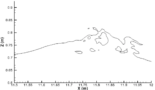
Once the front face of the crest steepens and becomes vertical (Fig. 4 a), a thin jet of water is indeed observed to be projected (Fig. 4 b). In the numerical results, the spilling phase thus starts as a very weak plunging breaking wave, with a small tongue of water thrown from the crest developing and free-falling down forward into a characteristic overturning motion. Once the jet is ejected from, it hits the water at the plunge point, very near to the crest of the wave. The plunging jet entraps a small gas pocket (Fig. 4 c). The resulting splash is directed down the wave leading to a spilling breaker (Fig. 4 d). White foam, consisting of a turbulent mixing of air bubbles and water (Fig. 3), should appear at the wave crest and spill down the front face of the propagating wave (Duncan 2001, Kimmoun and Branger 2007). However, compared with the 1 mm thick layer of foam initiating the experimental spilling wave from Kimmoun and Branger (2007), we observe numerically that the entrapped gas pockets are about 5 mm thick. For comparison, Fig. 4c shows the free-surface at corresponds to the experimental picture shown in Fig. 3. A good agreement between the free-surface topology can be seen, but the numerical picture only shows a single macro-bubble, instead of a white patch of small bubbles. The jet appearing at the wave crest at the early stage of the breaking initiation is clearly very small (Fig. 3b), about 1-cm high, but it is probably thicker than experimentally. This discrepancy has already been highlighted by Lubin et al. (2006b) and being attributed to numerical diffusion.
COASTAL ENGINEERING 2010 6 (a) (b) (c) (d)
Figure 4. Breaking wave evolution with velocity field in water. Tenth breaking wave spilling phase initiation. The free-surface profile corresponds to C = 0.5.
Then, the spilling breaker transitions in a strong plunging breaker. High velocities are located near the free-surface, due the jet-splash cycles, during the bore propagation. The free-surface is distorted and very dynamic (Fig. 5). The bore running-up the beach meets at some point the flow running-down from the previous broken wave.
Nevertheless, some differences appear again. Experimentally, air cavities entrapped during splash-up cycles are observed to be quickly fragmented into large plumes of bubbles (Miller 1976, Bonmarin 1989). The dislocation of the gas pockets into small bubbles cannot be simulated, even if, in the numerical results, the gas pockets correspond to some air-water mixing zones observed in the experimental pictures. The discrepancy is mainly due to the mesh grid resolution, which is still too coarse to be able to capture this flow feature. Indeed, the order of magnitude of bubble radii is usually
10−4 m (Dean and Stokes 2002), whereas our mesh grid resolution is xmin ≃ 5.10−4 m and
zmin≃ 1.25×10⁻³ m thanks to the dual grid used for the interface capturing. We are then able to track
the largest gas pockets and bubbles greater than 1 mm, as illustrated in Fig. 5 where a large variety of length scales can be observed. Turbulence is associated with air entrainment, which is responsible for wave energy damping in the surf zone. In the experiments, it appears that the entrained air bubbles are contained mostly in the large structures and diffused towards the bottom due to the eddies. The rate of energy dissipation is increased with the bubble penetration depth and strong vertical motions are induced by the rising air bubbles.
Figure 5. Breaking wave evolution with velocity field in water. Tenth breaking wave spilling phase initiation. The free-surface profile corresponds to C = 0.5.
Considering these simulations as a validation step, our numerical model gives very satisfactory and encouraging results for this 2D configuration.
Further efforts are required to increase the mesh grid resolution to improve the free-surface description and reduce the numerical diffusion. Parallel computations are now undertaken to reduce the calculation time.
CONCLUSIONS
We focused on describing the spilling phase of the experiments detailed by Kimmoun and Branger (2007). The numerical results presented in this paper concerns instantaneous quantities, simulating 2D regular waves breaking over a sloping beach. Our model was found to be reliable to describe correctly the complicated two-phase flow interactions that happen when waves break. The breaking process, in terms of wave overturning and splash-up occurrence, is in accordance with the general observations given in the literature. The air entrainment can be described, which is important as it plays a great role in the energy dissipation process. The interest of the numerical approach is to provide a complete and accurate description of free-surface and velocity evolutions in both air and water media during the
COASTAL ENGINEERING 2010 8
breaking of the waves, which must lead to the understanding of energy dissipation and turbulent flow structures generation processes. Nevertheless, wave breaking is a 3D two-phase turbulent problem, so the 2D numerical results presented here consisted in a first attempt.
Acknowledgements
The authors wish to thank the Aquitaine Regional Council for the financial support dedicated to a 256-processor cluster investment, located in the TREFLE laboratory. This work was granted access to the HPC resources of CINES under the allocation 2009-c2009026104 made by GENCI (Grand Equipement National de Calcul Intensif). The authors would like to acknowledge the financial and scientific support of the French INSU - CNRS (Institut National des Sciences de l’Univers - Centre National de la Recherche Scientifique) program IDAO (“Interactions et Dynamique de l’Atmosphère et de l’Océan”). This work was carried out under the project “Wave-induced circulation in the surf zone” coordinated by Dr. Hervé Michallet (LEGI - Grenoble).
REFERENCES
Battjes, A. 1988. Surf-zone dynamics. Ann. Rev. Fluid Mech., 20, 257-293.
Bonmarin, P. 1989. Geometric properties of deep-water breaking waves, J. Fluid Mech., 209, 405-433. Christensen, E. D., D. J. Walstra, and N. Emarat. 2002. Vertical variation of the flow across the surf
zone, Coastal Engineering, 45, 169-198.
Christensen, E. D. 2006. Large eddy simulation of spilling and plunging breakers, Coastal Engineering, 53, 463- 485.
Deane, G. B., and M. D. Stokes. 2002. Scale dependence of bubble creation mechanisms in breaking waves, Nature, 418, 839-844.
Duncan, J. H., 2001. Spilling breakers, Annu. Rev. Fluid Mech., 33, 519-547.
Fenton, J. D. 1985. A fifth-order Stokes theory for steady waves. Journal of Waterway, Port, Coastal and Ocean Engineering, 111, 216-234.
Helluy, P., F. Gollay, S. T. Grilli, N. Seguin, P. Lubin, J.-P. Caltagirone, S. Vincent, D. Drevard, and R. Marcer. 2005. Numerical simulations of wave breaking. Mathematical Modelling and Numerical Analysis Mathematical Modelling and Numerical Analysis, 39 (3), 591-608.
Kimmoun O., H. Branger, and B. Zucchini. 2004. Laboratory PIV measurements of wave breaking on a beach. Proceedings of 14th International Offshore and Polar Engineering Conference, 3, 293-298. Kimmoun K. and H. Branger. 2007. A PIV investigation on laboratory surf-zone breaking waves over a
sloping beach, J. Fluid Mech, 588, 353-397.
LeVeque, R. J. 1992. Numerical methods for conservation laws, Lectures in Mathematics, Birkhauser, Zurich.
Lin, P., and P. L.-F. Liu. 1999a. Free surface tracking methods and their applications to wave hydrodynamics, Vol. 5 of Advances in Coastal and Ocean Eng., World Scientific, 213-240. Lin, P., and P. L.-F. Liu. 1999b. Internal wave-maker for Navier-Stokes equations models, Journal of
Waterway, Port, Coastal and Ocean Engineering, 125, 322-330.
Lubin, P. 2004. Large eddy simulation of plunging breaking waves, PhD thesis (in English), University of Bordeaux.
Lubin, P., H. Branger, and O. Kimmoun. 2006a. Large eddy simulation of regular waves breaking over a sloping beach, Proceedings of 30th International Conference on Coastal Engineering, ASCE, 238-250.
Lubin, P., S. Vincent, S. Abadie and J.-P. Caltagirone. 2006b. Three-dimensional Large Eddy Simulation of air entrainment under plunging breaking waves, Coastal Engineering, 53, 631-655. Lubin, P., S. Glockner, and H. Chanson. 2010a. Numerical simulation of a weak breaking tidal bore,
Mechanics Research Communications, 37, 119-121.
Lubin, P., H. Chanson, and S. Glockner. 2010b. Large Eddy Simulation of turbulence generated by a weak breaking tidal bore, Environmental Fluid Mechanics, 10, 587-602.
Lubin, P., and J.-P. Caltagirone. 2010. Large eddy simulation of the hydrodynamics generated by breaking waves, in: Q. Ma (Ed.), Advances in numerical simulation of nonlinear water waves, Vol. 11 of Advances in Coastal and Ocean Engineering, World Scientific Publishing Company, Ch. 16, 575–604.
Miller, R. L. 1976. Role of vortices in surf zone prediction: sedimentation and wave forces, Soc. Econ. Paleontol. Mineral. Spec. Publ., 24, Ed. R. A. Davis, R. L. Ethington, 92-114.
Rudman, M. 1998. A volume-tracking method for incompressible multifluid flows with large density variations, Int. J. Numer. Meth. Fluids, 28, 357–378.
Sagaut, P. 1998. Large eddy simulation for Incompressible Flows, Springer, Verlag.
Sakaï, T., T. Mizutani, H. Tanaka and Y. Tada. 1986. Vortex formation in plunging breaker, Proceedings of 20th International Conference on Coastal Engineering, ASCE, 711-723.
Vincent, S., J.-P. Caltagirone, P. Lubin and T. N. Randrianarivelo. 2003. An adaptative augmented Lagrangian method for three-dimensional multi-material flows, Computers and Fluids, 33, 1273-1289.
Watanabe, Y., H. Saeki and R. J. Hosking. 2005. Three-dimensional vortex structures under breaking waves, J. Fluid Mech., 545, 291-328.