Counterfactual: An R Package for Counterfactual Analysis

(1)

The MIT Faculty has made this article openly available.

Please share

how this access benefits you. Your story matters.

Citation

Chen, Mingli et al. "Counterfactual: An R Package forCounterfactual

Analysis." The R Journal 9 (June 2017): 370-384 © 2017 Publisher

As Published

http://dx.doi.org/10.32614/rj-2017-033

Publisher

The R Foundation

Version

Final published version

Citable link

https://hdl.handle.net/1721.1/122790

Terms of Use

Creative Commons Attribution 4.0 International license

(2)

Counterfactual: An R Package for

Counterfactual Analysis

by Mingli Chen, Victor Chernozhukov, Iván Fernández-Val and Blaise Melly

Abstract The Counterfactual package implements the estimation and inference methods of Cher-nozhukov et al.(2013) for counterfactual analysis. The counterfactual distributions considered are the result of changing either the marginal distribution of covariates related to the outcome variable of interest, or the conditional distribution of the outcome given the covariates. They can be applied to estimate quantile treatment effects and wage decompositions. This paper serves as an introduction to the package and displays basic functionality of the commands contained within.

Introduction

Using econometric terminology, we can often think of a counterfactual distribution as the result of a change in either the distribution of a set of covariates X that determine the outcome variable of interest Y, or the relationship of the covariates with the outcomes, that is, a change in the conditional distribution of Y given X. Counterfactual analysis consists of evaluating the effects of such changes. TheCounterfactualpackage implements the methods of (Chernozhukov et al.,2013) for counterfactual analysis. It contains commands to estimate and make inference on quantile effects constructed from counterfactual distributions. The counterfactual distributions are estimated using regression methods such as classical, duration, quantile and distribution regressions. The inference on the quantile effect function can be pointwise at a specific quantile index or uniform over a range of specified quantile indexes.

We start by giving a simple example of counterfactual analysis. Suppose we would like to analyze the wage differences between men and women. Let 0 denote the population of men and let 1

denote the population of women. The variable Yjdenotes wages and Xjdenotes job market-relevant

characteristics that affect wages for populations j=0 and j=1. The conditional distribution functions

FY0|X0(y|x)and FY1|X1(y|x)describe the stochastic assignment of wages to workers with characteristics

x, for men and women, respectively. Let F_Yh0|0iand F_Yh1|1irepresent the observed distribution function

of wages for men and women, and let F_Yh0|1irepresent the distribution function of wages that would

have prevailed for women had they faced the men’s wage schedule F_Y₀_|X₀:

F_Yh0|1i(y):=

Z

X1

F_Y₀_|X₀(y|x)dFX1(x).

The latter distribution is called counterfactual, since it does not arise as a distribution from any observ-able population. Rather, this distribution is constructed by integrating the conditional distribution of wages for men with respect to the distribution of characteristics for women. This quantity is well

defined ifX₀, the support of men’s characteristics, includesX₁, the support of women’s characteristics,

namelyX₁⊂ X₀.

Let F←denote the quantile or left-inverse function of the distribution function F. The difference in

the observed wage quantile function between men and women can be decomposed in the spirit of (Oaxaca,1973) and (Blinder,1973) as

F_Yh1|1i← −F_Yh0|0i← = [F_Yh1|1i← −F_Yh0|1i← ] + [F_Yh0|1i← −F_Yh0|0i← ], (1) where the first term in brackets is due to differences in the wage structure and the second term is a composition effect due to differences in characteristics. These counterfactual effects are well defined econometric parameters and are widely used in empirical analysis, for example, the first term of the

decomposition is a measure of gender wage discrimination. In Section2.3.2we consider an empirical

example where 0 denotes the population of nonunion workers and 1 denotes the population of union workers. In this case the the wage structure effect corresponds to the treatment effect of union or union premium. It is important to note that these effects do not necessarily have a causal interpretation

(3)

The Counterfactual package

Getting started

To get started using the package Counterfactual for the first time, issue the command > install.packages("Counterfactual")

into your R browser to install the package in your computer. Once the package has been installed, you can use the package Counterfactual during any R session by simply issuing the command

> library(Counterfactual)

Now you are ready to use the function counterfactual and data sets contained in Counterfactual. For general questions about the package you may type

> help(package = "Counterfactual")

to view the package help file, or for more questions about a specific function you can type ‘help(function-name)’. For example, try:

> help(counterfactual) or simply type

> ?counterfactual

The command counterfactual has the general syntax:

> counterfactual(formula, data, weights, na.action = na.exclude,

+ group, treatment = FALSE, decomposition = FALSE,

+ transformation = FALSE, counterfactual_var,

+ quantiles, method = "qr",

+ trimming = 0.005, nreg = 100, scale_variable,

+ counterfactual_scale_variable,

+ censoring = 0, right = FALSE, nsteps = 3,

+ firstc = 0.1, secondc = 0.05, noboot = FALSE,

+ weightedboot = FALSE, seed = 8, robust = FALSE,

+ reps = 100, alpha = 0.05, first = 0.1,

+ last = 0.9, cons_test = 0, printdeco = TRUE,

+ sepcore = FALSE, ncore=1)

To describe the different options of the command we need to provide some background on methods for counterfactual analysis.

Setting for counterfactual analysis

Consider a general setting with two populations labeled by k∈ K = {0, 1}. For each population k

there is the dx-vector Xkof covariates and the scalar outcome Yk. The covariate vector is observable

in all populations, but the outcome is only observable in populations j∈ J ⊆ K. Let FXkdenote the

covariate distribution in population k∈ K, and FYj|Xjand QYj|Xjdenote the conditional distribution

and quantile functions in population j∈ J. We denote the support of XkbyXk⊆Rdx, and the region

of interest for YjbyYj⊆R. The refer to j as the reference population(s) and to k as the counterfactual

population(s).

The reference and counterfactual populations in the wage examples correspond to different groups such as men and women or nonunion and union workers. We can also generate counterfactual

populations by artificially transforming a reference population. Formally, we can think of Xkas being

created through a known transformation of Xj:

Xk=gk(Xj), where gk:Xj→ Xk. (2)

This case covers adding one unit to the first covariate, X1,k=X1,j+1, holding the rest of the covariates

constant. The resulting quantile effect becomes the unconditional quantile regression, which measures the effect of a unit change in a given covariate component on the unconditional quantiles of Y. For example, this type of counterfactual is useful for estimating the treatment effect of smoking during pregnancy on infant birth weights. Another possible transformation is a mean preserving

(4)

general types of transformation defined in (2) are useful for estimating the effect of a change in taxation on the marginal distribution of food expenditure or the effect of cleaning up a local hazardous waste

site on the marginal distribution of housing prices ((Stock,1991)). We give an example of this type of

transformation in Section2.3.1.

The reference and counterfactual populations can be specified to counterfactual in two ways that accommodate the previous two cases:

1. If the option group has been specified, then j is the population defined by group and k is the population defined by group=1. This means that both X and Y are observed in group=0, but only X needs to be observed in group=1. When both X and Y are observed in group=1, the option treatment=TRUE specifies that the structure or treatment effect should be computed, whereas the default option treatment=FALSE specifies that the composition effect should be

computed; see the definition of the structure and composition effects in the decomposition (1).

If in addition to treatment=TRUE the option decomposition=TRUE is selected, then the entire

decomposition (1) is reported including the composition, structure and total effects. Note that

we can reverse the roles of the populations defined by an indicator variable vargroup by setting either group=vargroup or group=1-vargroup.

2. Alternatively, the option counterfactual_var can be used to specify the covariates in the counter-factual population. In this case, the names on the right handside of formula contain the variables

in Xjand counterfactual_var contains the variables in Xk. The option transformation=TRUE should

be used when Xkis generated as a transformation of Xj, e.g., equation (2). The list passed to

counterfactual_var must contain exactly the same number of variables as the list of independent variables in formula and the order of the variables in the list matters.

Counterfactual distribution and quantile functions are formed by combining the conditional distribution in the population j with the covariate distribution in the population k, namely:

FYhj|ki(y):=

R

XkFYj|Xj(y|x)dFXk(x), y∈ Yj, Q_Yhj|ki(τ):=F_Yhj|ki← (τ), τ∈ (0, 1),

where(_{j, k}) ∈ J K, and F_Yhj|ki← (τ) = inf{y ∈ Yj : FYhj|ki(y) ≥ τ}is the left-inverse function of

F_Yhj|ki. The main interest lies in the quantile effect (QE) function, defined as the difference of two

counterfactual quantile functions over a set of quantile indexesT ⊂ (0, 1):

∆(τ) =QYhj|ki(τ) −QYhj|ji(τ), τ∈ T,

where j∈ J and k∈ K. In the example of Section2.1, we obtain the composition effect with j=0

and k=1. When Ykis observed, then we can construct the structure effect or treatment effect on the

treated

∆(τ) =Q_Yhk|ki(τ) −Q_Yhj|ki(τ), τ∈ T,

by specifying the option group and setting treatment=TRUE. In the example of Section2.1, we obtain

the wage structure effect with j=0 and k=1, i.e. setting group=1 and treatment=TRUE. If in addition

we select the option decomposition=TRUE, then we obtain the entire decomposition (1) including the

composition, structure and total effects. The total effect is

∆(τ) =Q_Yhk|ki(τ) −Q_Yhj|ji(τ), τ∈ T.

The setT is specified with the option quantiles, which enumerates the quantile indexes of interested

and should be a vector containing numbers between 0 and 1.

To estimate the QE function we need to model and estimate the conditional distribution FYj|Xjand

covariate distribution FXk. We estimate the covariate distribution using the empirical distribution,

and consider several regression based methods for the conditional distribution including classical, quantile, duration, and distribution regression. Given the estimators of the conditional and covariate

distributions ˆF_Y_j_|X_jand ˆFXk, the estimator of each counterfactual distribution is obtained by the plug-in

rule, namely ˆ F_Yhj|ki(y) = Z Xk ˆ F_Y_j_|X_j(y|x)d ˆFXk(x), y∈ Yj.

Then, the estimator of the QE function is also obtained by the plug-in rule as ˆ

∆(τ) =Fˆ_Yhj|ki← (τ) −Fˆ_Yhj|ji← (τ), τ∈ T, or

ˆ

(5)

if we define the counterfactual population with group and set treatment=TRUE. If in addition to treatment=TRUE, we select decomposition=TRUE, then the plug-in estimator of the total effect is

ˆ

∆(τ) =Fˆ_Yhk|ki← (τ) −Fˆ_Yhj|ji← (τ), τ∈ T.

Estimation of conditional distribution

In this section we assume that we have samples{(Yji, Xji): i=1, . . . , nj}composed of independent

and identically distributed copies of(Yj, Xj)for all populations j∈ J. The conditional distribution

F_Y_j_|X_j can be modeled and estimated directly, or throught the conditional quantile function, Q_Y_j_|X_j,

using the relation

FYj|Xj(y|x) ≡

Z

(0,1)1{QYj|Xj

(u|x) ≤y}du. (3) The option formula specifies the outcome Y as the left hand side variable and the covariates X as the right hand side variable(s). The option method allows to select the method to estimate the conditional distribution. The following methods are implemented:

1. method = "qr", which is the default, implements the quantile regresion estimator of the condi-tional distribution ˆ F_Y_j_|X_j(y|x) =ε+ Z (ε,1−ε)1 {x0ˆβj(u) ≤y}du, (4)

where ε is a small constant that avoids estimation of tail quantiles, and ˆβ(u)is the (Koenker and

Bassett,1978) quantile regression estimator

ˆβj(u) =arg min b∈Rdx nj

∑

i=1 [u−1{Yji≤X0jib}][Yji−X0jib].

The quantile regression estimator calls the R packagequantreg(Koenker,2016). The option

trimming specifies the value of the trimming parameter ε, with default value ε=0.005. The

option nreg sets the number of quantile regressions used to approximate the integral in (4), with a

default value of 100 such that(ε, 1−ε)is approximated by the grid{ε, ε+ (1−2ε)/99, ε+2(1−

2ε)/99, . . . , 1−ε}. This method should be used only with continuous dependent variables.

2. method = "loc" implements the estimator of the conditional distribution ˆ F_Y_j_|X_j(y|x) = 1 nj nj

∑

i=1 1{Yji−X0jiˆβj≤y−x0ˆβj}, (5)

where ˆβjis the least square estimator

ˆβj=arg min b∈Rdx nj

∑

i=1 (Yji−X0jib)2. (6)

The estimator (5) is based on a restrictive location shift model that imposes that the covariates X

only affect the location of the outcome Y.

3. method = "locsca" implements the estimator of the conditional distribution ˆ F_Y_j_|X_j(y|x) = 1 nj nj

∑

i=1 1 ( Yji−X0jiˆβj exp(X_2ji0 γˆj/2) ≤ y−x 0_ˆβ j exp(x_2j0 γˆj/2) ) , (7)

where ˆβjis the least square estimator (6), X2j⊆Xjwith dim X2j=dx2, and

ˆ γj=arg min g∈Rdx2 nj

∑

i=1 (log(Yji−X0jiˆβj)2−X02jig)2.

The option scale_variable specifies the covariates X2jthat affect the scale of the conditional

distribution. The option counterfactual_scale_variable selects the counterfactual scale variables when the counterfactual population is specified using counterfactual_var. By default, R would use all the covariates as scale_variable and counterfactual_scale_variable = counterfactual_var. The

estimator (7) is based on a restrictive location scale shift model that imposes that the covariates

X only affect the location and scale of the outcome Y.

4. method = "cqr" implements the censored quantile regression estimator of the conditional

(6)

censored quantile regression estimator. The options trimming and nreg apply to this method with the same functionality as for the qr method. Moreover, a variable containing a censoring

indicator Cjmust be specified with censoring. The censored quantile regression estimator has

three-steps by default. The number of steps can be increased by the option nsteps. In the first step, the censoring probabilities are estimated by a logit regression of the censoring indicator

Cjon all the covariates Xj. Then, for each quantile index u, the observations with sufficiently

low censoring probabilities relative to u are selected. We allow for misspecification of the logit by excluding the observations that could theoretically be used but have censoring probabilities in the highest firstc quantiles, with a default of 0.1, i.e. 10% of the observations. In the second step, standard linear quantile regressions are estimated on the samples defined in step one. Using the estimated quantile regressions, we define a new sample of observations that can be used. This sample consists of all observations for which the estimated conditional quantile is above the censoring point. Again, we throw away observations in the lowest secondc quantiles of the distribution of the residuals, with a default of 0.05, i.e. 5% of the observations. Step three consists in a new linear quantile regression using the sample defined in step two. Step three is repeated if nsteps is above 3. This method should be used only with censored dependent variables.

5. method = "cox" implements the duration regression estimator of the conditional distribution function

ˆ

F_Y_j_|X_j(y|x) =1−exp(−exp(ˆt(y) −x0ˆβ)), (8)

where ˆβ is the Cox estimator of the regression coefficients and ˆt(y)is the Cox estimator of the

baseline integrated hazard function (Cox,1972). The Cox estimator calls the R packagesurvival

(Therneau,2015). The estimator (8) is based on a restrictive transformation location shift model that imposes that the covariates X only affect the location of a monotone transformation of the

outcome t(Y), i.e.

t(Yj) =X0jβj+Vj,

where Vjhas an extreme value distribution and is independent of Xj. This method should be

used only with nonnegative dependent variables.

6. method = "logit" implements the distribution regression estimator of the conditional distribution with logistic link function

ˆ

F_Y_j_|X_j(y|x) =Λ(x0ˆβ(y)), (9)

whereΛ is the standard logistic distribution function, and ˆβ(y)is the distribution regression

estimator ˆβ(y) =arg max b∈Rdx nj

∑

i=1 h 1{Yji≤y}logΛ(Xij0b) +1{Yij>y}logΛ(−X0jib) i . (10)

The estimator (9) is based on a flexible model where each covariate can have a heterogenous

effect at different parts of the distribution. This method can be used with continuous dependent variables and censored dependent variables with fixed censoring point.

7. method = "probit" implements the distribution regression estimator of the conditional distribution

with normal link function, i.e. whereΛ is the standard normal distribution function in (9) and

(10).

8. method = "lpm" implements the linear probability model estimator of the conditional distribution ˆ

F_Y_j_|X_j(y|x) =x0ˆβ(y),

where ˆβ(y)is the least squares estimator

ˆβ(y) =arg min b∈Rdx nj

∑

i=1 (1{Yji≤y} −Xij0b)2.

This method might produce estimates of the conditional distribution outside the interval[0, 1].

For the methods (2)–(8), the option nreg sets the number of values of y to evaluate the estimator of the conditional distribution function. These values are uniformly distributed among the observed

values of Yj. If nreg is greater than the number of observed values of Yj, then all the observed values

(7)

Inference

The command counterfactual reports pointwise and uniform confidence intervals for the QEs over a prespecified set of quantile indexes. The construction of the intervals rely on functional central limit theorems and bootstrap functional central limit theorems for the empirical QEs derived in (Chernozhukov et al.,2013). In particular, the pointwise intervals are based on the normal distribution, whereas the uniform intervals are based on two resampling schemes: empirical and weighted bootstrap.

Thus, the(1−α)confidence interval for∆(τ)onT has the form

{_∆ˆ(τ) ±c1−αΣˆ(τ): τ∈ T },

where ˆΣ(τ)is the standard error of ˆ∆(τ)and c1−αis a critical value. There are two options to obtain

ˆ

Σ(τ). The default option robust=FALSE computes the bootstrap standard deviation of ˆ∆(τ); whereas

the option robust=TRUE computes the bootstrap interquartile range rescaled with the normal

distribu-tion, ˆΣ(τ) = (q0.75(τ) −q0.25(τ))/(z0.75−z0.25)where qp(τ)is the pth quantile of the bootstrap draws

of ˆ∆(τ)and zpis the pth quantile of the standard normal. The pointwise critical value is c1−α=z1−α,

and the uniform critical value is c1−α = ˆt1−α, where ˆt1−αis a bootstrap estimator of the(1−α)th

quantile of the Kolmogorov-Smirnov maximal t-statistic

t=sup

τ∈T

|_∆ˆ(τ) −∆(τ)|/ ˆΣ(τ).

In addition to the intervals, counterfactual reports the p-values for several functional tests based on two test-statistic: Kolmogorov-Smirnov and the Cramer-von-Misses-Smirnov. The null-hypotheses considered are

1. Correct parametric specification of the model for the conditional distribution. This test compares

the empirical distribution of the outcome Yjwith the estimate of the counterfactual distribution

in the reference population ˆ F_Yhj|ji(y):= Z Xj ˆ F_Y_j_|X_j(y|x)d ˆFXj(x).

The power of this specification test might be low because it only uses the implications of the conditional distribution on the counterfactual distribution. For example, the test is not informative for the linear probability and logit models where the counterfactual distribution in the reference population is identical to the empirical distribution by construction. If group is specified and treatment=TRUE is selected, then the test is performed in the population defined by group=1. If in addition the option decomposition=TRUE is selected, then the test is performed in the populations defined by group=0 and group=1, and in the combined population including both group=0 and group=1.

2. Zero QE at all the quantile indexes of interest:∆(τ) =0 for all τ∈ T. This is stronger than a

zero average effect. Other null hypotheses of constant quantile effect (but at a different level than 0) can be added with the option cons_test.

3. Constant QE at all quantile indexes of interest:∆(τ) =∆(0.5)for all τ∈ T.

4. First-order stochastic dominance:∆(τ) ≥0 for all τ∈ T.

5. Negative first-order stochastic dominance:∆(τ) ≤0 for all τ∈ T.

The options of counterfactual related to inference are:

1. noboot = TRUE suppresses the bootstrap. The bootstrap can be very demanding in terms of computation time. Therefore, it is recommended to switch it off for the exploratory analysis of the data.

2. weightedboot = TRUE selects weighted bootstrap with standard exponential weights. The default weightedboot = FALSE selects empirical bootstrap with multinomial weights. We recommend weighted bootstrap when the covariates include categorical variables with small cell sizes to avoid singular designs in the bootstrap draws.

3. reps specifies the number of bootstrap replications. This number will matter only if the bootstrap has not be suppressed. The default is 100.

4. alpha specifies the significance level of the tests and confidence intervals. Note that the confidence level of the confidence interval is 1 - alpha. Thus, the default value of 0.05 produces 95% confidence intervals.

(8)

5. first and last select the subset of quantile indexes of interest for inference. The tails of the distribution should not be used because standard asymptotic does not apply to these parts. The needed amount of tail trimming depends on the sample size and on the distribution of the dependent variable. first sets the lowest quantile index used and last sets the highest quantile

index used. The default values are 0.1 and 0.9 so thatT = [0.1, 0.9].

6. cons_test add tests of the null hypothesis that∆(τ) =const_test for all τ between first and last.

The null hypothesis that∆(τ) =0 for all τ between first and last is tested by default. The null

hypothesis that the quantile effects are constant is also tested by default.

Parallel computing

The command counterfactual provides functionality for parallel computing, which is specially useful to speed up the execution of the bootstrap. There are two options related to parallel computing:

1. setcore specifies whether multiple cores should be used. The default value setcore = FALSE turns off the parallel computing.

2. ncore selects the number of cores to use for parallel computing. The information of this option is only used when parallel computing is switched on with setcore = TRUE.

Empirical examples

We consider two empirical examples to illustrate the functionality of the command counterfactual. The first example is an estimation of Engel curves that includes a counterfactual analysis where the counterfactual population is an artificial transformation of a reference population. The second example is wage decomposition with respect to union status where the reference and counterfactual populations correspond to two different groups.

Engel curves

We use the classical Engel 1857 dataset to estimate the relationship between food expenditure (foodexp) and annual household income (income), and then report the estimates of the QE of a change in the distribution of the annual household income that might be induced for example by a variation in

income taxation.1_{We estimate the conditional distribution with the quantile regression method, i.e.,}

method ="qr".

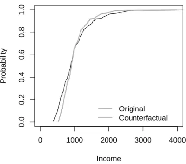
First, we generate the variable counterfactual_income with the counterfactual values of income and plot the reference and counterfactual income distributions. The counterfactual distribution corresponds to a mean preserving spread of the distribution in the reference population that reduces standard deviation by 25%. > library(quantreg) > data(engel) > attach(engel) > counter_income <- mean(income)+0.75*(income-mean(income)) > cdfx <- c(1:length(income))/length(income)

> plot(c(0,4000),range(c(0,1)), xlim =c(0, 4000), type="n", xlab = "Income",

+ ylab="Probability")

> lines(sort(income), cdfx)

> lines(sort(counter_income), cdfx, lwd = 2, col = 'grey70')

> legend(1500, .2, c("Original", "Counterfactual"), lwd=c(1,2),bty="n",

+ col=c(1,'grey70'))

To estimate the QEs of this counterfactual change we turn on the option transformation of counter-factual by setting transformation = TRUE, and specify that the countercounter-factual values of the covariate income are in the generated variable counter_income by setting counterfactual_var = counter_income. This yields:

> qrres <- counterfactual(foodexp~income, counterfactual_var

+ = counter_income, transformation = TRUE)

(9)

0 1000

2000

3000

4000

0.0

0.2

0.4

0.6

0.8

1.0 Income

Probability

Original

Counterfactual

Figure 1:Observed and counterfactual distributions of income

Conditional Model: linear quantile regression

Number of regressions estimated: 100

The variance has been estimated by bootstraping the results 100 times.

No. of obs. in the reference group: 235

No. of obs. in the counterfactual group: 235 Quantile Effects -- Composition

---Pointwise Pointwise Functional

Quantile Est. Std.Err 95% Conf.Interval 95% Conf.Interval

0.1 68.049 4.214 59.789 76.308 55.939 80.159 0.2 57.897 4.332 49.406 66.388 45.448 70.346 0.3 43.851 5.246 33.568 54.133 28.774 58.927 0.4 29.248 5.091 19.270 39.227 14.618 43.878 0.5 16.716 4.602 7.696 25.735 3.491 29.940 0.6 5.744 4.308 -2.698 14.187 -6.634 18.123 0.7 -8.866 7.132 -22.845 5.113 -29.361 11.630 0.8 -40.099 8.191 -56.153 -24.045 -63.637 -16.561 0.9 -88.56 13.83 -115.67 -61.44 -128.31 -48.80

Bootstrap inference on the counterfactual quantile process

---P-values

======================

NULL-Hypthoesis KS-statistic CMS-statistic

======================================================================

Correct specification of the parametric model 0 0

No effect: QE(tau)=0 for all taus 0 0

Constant effect: QE(tau)=QE(0.5) for all taus 0 0

Stochastic dominance: QE(tau)>0 for all taus 0 0

(10)

We reject the simultaneous hypotheses of zero, constant, positive and negative effect of the income redistribution at all the deciles. The QR model for the conditional distribution cannot be rejected at conventional significance levels.

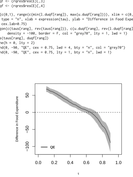
Finally, we reestimate the QE function on the larger set of quantiles{0.01, 0.02, . . . , 0.99}, and plot

a uniform confidence band over the subset{0.10, 0.11, . . . , 0.90}constructed by empirical bootstrap

with 100 replications. In Figure2we can visually reject the functional hypotheses of zero, constant,

positive and negative effect at the percentiles considered. We use the option printdeco = FALSE to suppress the display of the table of results.

> taus <- c(1:99)/100

> first <- sum(as.double(taus <= .10)) > last <- sum(as.double(taus <= .90)) > rang <- c(first:last)

> rqres <- counterfactual(foodexp~income, counterfactual_var=counter_income,

+ nreg=100, quantiles=taus, transformation = TRUE,

+ printdeco = FALSE, sepcore = TRUE,ncore=2)

cores used= 2

> duqf <- (rqres$resCE)[,1]

> l.duqf <- (rqres$resCE)[,3] > u.duqf <- (rqres$resCE)[,4]

> plot(c(0,1), range(c(min(l.duqf[rang]), max(u.duqf[rang]))), xlim = c(0,1),

+ type = "n", xlab = expression(tau), ylab = "Difference in Food Expenditure",

+ cex.lab=0.75)

> polygon(c(taus[rang], rev(taus[rang])), c(u.duqf[rang], rev(l.duqf[rang])),

+ density = -100, border = F, col = "grey70", lty = 1, lwd = 1)

> lines(taus[rang], duqf[rang]) > abline(h = 0, lty = 2)

> legend(0, -90, "QE", cex = 0.75, lwd = 4, bty = "n", col = "grey70") > legend(0, -90, "QE", cex = 0.75, lty = 1, bty = "n", lwd = 1)

0.0

0.2

0.4

0.6

0.8

1.0 −100

−50

0

50

τ Diff erence in F ood Expenditure QE QE

(11)

Union premium

We use an extract of the U.S. National Longitudinal Survey of Young Women (NLSW) for employed

women in 1988 to estimate a wage decomposition with respect to union status.2 The outcome variable

Y is the log hourly wage (lwage), the covariates X include job tenure in years (tenure), years of schooling (grade), and total experience (ttl_exp), and the union indicator union defines the reference and counterfactual populations. We estimate the conditional distributions by distribution regression with logistic link and duration regression, i.e., method ="logit" and method ="cox". We use weighted bootstrap for the construction of uniform confidence intervals and hypothesis tests and run parallel computing with 2 nodes.

We start by estimating the wage decomposition by logistic distribution regression, where the counterfactual population is specified with group=union with the options treatment=TRUE and decom-position=TRUE to estimate the composition, structure and total effects. The structure effect in this case correspond to the treatment effect of union on the treated or union premium. The tables show that the union workers earn higher wages than the nonumion workers throuoghout the distribution although the union wage gap is decreasing in the quantile index. This gap can be mostly explained by differences in tenure, education and experience between union and nonunion workers in the upper tail of the distribution and by the union premium in the rest of the distribution.

> data(nlsw88) > attach(nlsw88)

> lwage <- log(wage)

> logitres <- counterfactual(lwage~tenure+ttl_exp+grade,

+ group = union, treatment=TRUE,

+ decomposition=TRUE, method = "logit",

+ weightedboot = TRUE, sepcore = TRUE, ncore=2)

cores used= 2

Conditional Model: logit

Number of regressions estimated: 96

The variance has been estimated by bootstraping the results 100 times.

No. of obs. in the reference group: 1407

No. of obs. in the counterfactual group: 459 Quantile Effects -- Structure

0.1 0.24047 0.06005 0.12278 0.35817 0.07757 0.40338 0.2 0.21903 0.05630 0.10869 0.32937 0.06631 0.37176 0.3 0.23437 0.04628 0.14366 0.32508 0.10881 0.35992 0.4 0.18524 0.04252 0.10190 0.26857 0.06989 0.30059 0.5 0.16041 0.04404 0.07410 0.24671 0.04095 0.27987 0.6 0.13897 0.04618 0.04845 0.22949 0.01369 0.26425 0.7 0.05701 0.04407 -0.02937 0.14339 -0.06255 0.17657 0.8 0.01945 0.04179 -0.06245 0.10135 -0.09391 0.13281 0.9 0.006434 0.078547 -0.147514 0.160382 -0.206650 0.219518 Bootstrap inference on the counterfactual quantile process

---P-values

======================

======================================================================

Constant effect: QE(tau)=QE(0.5) for all taus 0 0.02

Stochastic dominance: QE(tau)>0 for all taus 0.95 0.95

(12)

Stochastic dominance: QE(tau)<0 for all taus 0 0 Quantile Effects -- Composition

0.1 0.06062 0.04131 -0.02035 0.14160 -0.05752 0.17877 0.2 0.04879 0.03717 -0.02406 0.12164 -0.05750 0.15508 0.3 0.05313 0.03721 -0.01981 0.12607 -0.05329 0.15956 0.4 0.09245 0.03772 0.01851 0.16638 -0.01543 0.20033 0.5 0.08952 0.03945 0.01220 0.16683 -0.02329 0.20233 0.6 0.12259 0.03862 0.04690 0.19828 0.01215 0.23303 0.7 0.12975 0.03781 0.05564 0.20385 0.02162 0.23787 0.8 0.090722 0.030184 0.031563 0.149881 0.004404 0.177041 0.9 0.05503 0.05744 -0.05755 0.16760 -0.10924 0.21929

---P-values

======================

======================================================================

No effect: QE(tau)=0 for all taus 0.01 0.01

Constant effect: QE(tau)=QE(0.5) for all taus 0.77 0.58

Stochastic dominance: QE(tau)<0 for all taus 0.01 0.01

Quantile Effects -- Total

0.1 0.30110 0.05703 0.18933 0.41287 0.13655 0.46565 0.2 0.26782 0.06383 0.14271 0.39293 0.08363 0.45202 0.3 0.28750 0.05459 0.18051 0.39449 0.12998 0.44502 0.4 0.27768 0.05211 0.17556 0.37981 0.12733 0.42804 0.5 0.24992 0.05111 0.14975 0.35010 0.10244 0.39741 0.6 0.26156 0.04999 0.16358 0.35953 0.11731 0.40580 0.7 0.18675 0.04529 0.09800 0.27551 0.05608 0.31743 0.8 0.11017 0.04624 0.01954 0.20081 -0.02327 0.24361 0.9 0.06146 0.06287 -0.06176 0.18468 -0.11996 0.24287

---P-values

======================

======================================================================

Constant effect: QE(tau)=QE(0.5) for all taus 0.06 0.13

Stochastic dominance: QE(tau)<0 for all taus 0 0

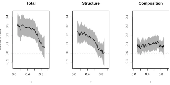
Next, we reestimate the QE function on the larger set of quantiles{0.01, 0.02, ..., 0.99}, and plot a

uniform confidence band over the subset{0.10, 0.11, ..., 0.90}) constructed by weighted bootstrap with

100 replications. Figure3shows that the structure effect is heterogeneous across the quantile indexes

and explains most of the union wage gap below the third quartile. The composition effect is constant across quantile indexes and explains most of the wage gap above the third quartile.

(13)

> first <- sum(as.double(taus <= .10)) > last <- sum(as.double(taus <= .90)) > rang <- c(first:last)

> logitres <- counterfactual(lwage~tenure+ttl_exp+grade,

+ group = union, treatment=TRUE, quantiles=taus,

+ method="logit", nreg=100, weightedboot = TRUE,

+ printdeco=FALSE, decomposition = TRUE,

+ sepcore = TRUE,ncore=2) cores used= 2 > duqf_SE <- (logitres$resSE)[,1] > l.duqf_SE <- (logitres$resSE)[,3] > u.duqf_SE <- (logitres$resSE)[,4] > duqf_CE <- (logitres$resCE)[,1] > l.duqf_CE <- (logitres$resCE)[,3] > u.duqf_CE <- (logitres$resCE)[,4] > duqf_TE <- (logitres$resTE)[,1] > l.duqf_TE <- (logitres$resTE)[,3] > u.duqf_TE <- (logitres$resTE)[,4]

> range_x <- min(c(min(l.duqf_SE[rang]), min(l.duqf_CE[rang]),

+ min(l.duqf_TE[rang])))

> range_y <- max(c(max(u.duqf_SE[rang]), max(u.duqf_CE[rang]),

+ max(u.duqf_TE[rang])))

> par(mfrow=c(1,3))

> plot(c(0,1), range(c(range_x, range_y)), xlim = c(0,1), type = "n",

+ xlab = expression(tau), ylab = "Difference in Wages", cex.lab=0.75,

+ main = "Total")

> polygon(c(taus[rang],rev(taus[rang])),

+ c(u.duqf_TE[rang], rev(l.duqf_TE[rang])), density = -100, border = F,

+ col = "grey70", lty = 1, lwd = 1)

> lines(taus[rang], duqf_TE[rang]) > abline(h = 0, lty = 2)

+ xlab = expression(tau), ylab = "", cex.lab=0.75, main = "Structure")

+ c(u.duqf_SE[rang], rev(l.duqf_SE[rang])), density = -100, border = F,

+ col = "grey70", lty = 1, lwd = 1)

> lines(taus[rang], duqf_SE[rang]) > abline(h = 0, lty = 2)

+ xlab = expression(tau), ylab = "", cex.lab=0.75, main = "Composition")

+ c(u.duqf_CE[rang], rev(l.duqf_CE[rang])), density = -100, border = F,

+ col = "grey70", lty = 1, lwd = 1)

> lines(taus[rang], duqf_CE[rang]) > abline(h = 0, lty = 2)

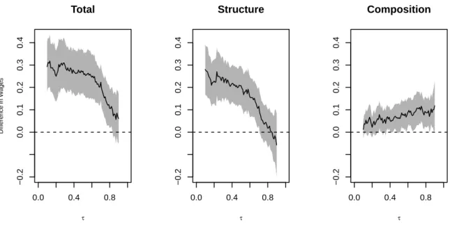
Finally, we repeat the point and interval estimation using the duration regression method with the option method = "cox". Despite of relying on a more restrictive model for the conditional distribution,

the duration regression estimates in Figure4are similar to the logit regression estimates in Figure3.

> coxres <- counterfactual(lwage~tenure+ttl_exp+grade,

+ group = union, treatment=TRUE, quantiles=taus,

+ method="cox", nreg=100, weightedboot = TRUE,

+ printdeco = FALSE, decomposition = TRUE, sepcore = TRUE,ncore=2)

cores used= 2 > duqf_SE <- (coxres$resSE)[,1] > l.duqf_SE <- (coxres$resSE)[,3] > u.duqf_SE <- (coxres$resSE)[,4] > duqf_CE <- (coxres$resCE)[,1] > l.duqf_CE <- (coxres$resCE)[,3] > u.duqf_CE <- (coxres$resCE)[,4] > duqf_TE <- (coxres$resTE)[,1] > l.duqf_TE <- (coxres$resTE)[,3]

(14)

0.0 0.4 0.8 −0.1 0.0 0.1 0.2 0.3 0.4

Total

τ Diff erence in W ages 0.0 0.4 0.8 −0.1 0.0 0.1 0.2 0.3 0.4

Structure

τ 0.0 0.4 0.8 −0.1 0.0 0.1 0.2 0.3 0.4

Composition

τ

Figure 3:Wage decomposition with respect to union: logit regression estimates

> u.duqf_TE <- (coxres$resTE)[,4]

> range_x = min(c(min(l.duqf_SE[rang]), min(l.duqf_CE[rang]),

+ min(l.duqf_TE[rang])))

> range_y = max(c(max(u.duqf_SE[rang]), max(u.duqf_CE[rang]),

+ max(u.duqf_TE[rang])))

> par(mfrow=c(1,3))

+ xlab = expression(tau), ylab = "Difference in Wages", cex.lab=0.75,

+ main = "Total")

+ c(u.duqf_TE[rang], rev(l.duqf_TE[rang])), density = -100, border = F,

+ col = "grey70", lty = 1, lwd = 1)

> lines(taus[rang], duqf_TE[rang]) > abline(h = 0, lty = 2)

+ xlab = expression(tau), ylab = " ", cex.lab=0.75, main = "Structure")

+ c(u.duqf_SE[rang], rev(l.duqf_SE[rang])), density = -100, border = F,

+ col = "grey70", lty = 1, lwd = 1)

> lines(taus[rang], duqf_SE[rang]) > abline(h = 0, lty = 2)

+ xlab = expression(tau), ylab = "", cex.lab=0.75, main = "Composition")

+ c(u.duqf_CE[rang], rev(l.duqf_CE[rang])), density = -100, border = F,

+ col = "grey70", lty = 1, lwd = 1)

> lines(taus[rang], duqf_CE[rang]) > abline(h = 0, lty = 2)

Bibliography

A. Blinder. Wage discrimination: Reduced form and structural estimates. Journal of Human resources,

pages 436–455, 1973. [p370]

V. Chernozhukov and H. Hong. Three-step censored quantile regression and extramarital affairs.

(15)

0.0 0.4 0.8 −0.2 0.0 0.1 0.2 0.3 0.4

Total

τ Diff erence in W ages 0.0 0.4 0.8 −0.2 0.0 0.1 0.2 0.3 0.4

Structure

τ 0.0 0.4 0.8 −0.2 0.0 0.1 0.2 0.3 0.4

Composition

τ

Figure 4:Wage decomposition with respect to union: duration regression estimates

V. Chernozhukov, I. Fernández-Val, and B. Melly. Inference on counterfactual distributions.

Economet-rica, 81(6):2205–2268, 2013. [p370,375]

D. R. Cox. Regression models and life-tables. Journal of the Royal Statistical Society B, 34(2):187–220,

1972. [p374]

R. Koenker. Quantreg: Quantile Regression, 2016. URLhttps://CRAN.R-project.org/package=

quantreg. R package version 5.21. [p373,376]

R. Koenker and G. Bassett. Regression quantiles. Econometrica: journal of the Econometric Society, pages

33–50, 1978. [p373]

R. Oaxaca. Male-female wage differentials in urban labor markets. International economic review, pages

693–709, 1973. [p370]

J. Stock. Nonparametric policy analysis: An application to estimating hazardous waste cleanup benefits. Nonparametric and Semiparametric Methods in Econometrics and Statistics, pages 77–98, 1991.

[p372]

T. M. Therneau. A Package for Survival Analysis in S, 2015. URLhttp://CRAN.R-project.org/package=

survival. version 2.38. [p374] Mingli Chen Department of Economics University of Warwick UK m.chen.3@warwick.ac.uk Victor Chernozhukov Department of Economics

Massachusetts Institute of Technology USA vchern@mit.edu Iván Fernández-Val Department of Economics Boston University USA ivanf@bu.edu

(16)

Blaise Melly

Department of Economics University of Bern Germany