HAL Id: hal-01159676
https://hal.inria.fr/hal-01159676
Submitted on 3 Jun 2015
HAL is a multi-disciplinary open access
archive for the deposit and dissemination of
sci-entific research documents, whether they are
pub-lished or not. The documents may come from
L’archive ouverte pluridisciplinaire HAL, est
destinée au dépôt et à la diffusion de documents
scientifiques de niveau recherche, publiés ou non,
émanant des établissements d’enseignement et de
Hypergraph partitioning for multiple communication
cost metrics: Model and methods
Mehmet Deveci, Kamer Kaya, Bora Uçar, Umit Catalyurek
To cite this version:
Mehmet Deveci, Kamer Kaya, Bora Uçar, Umit Catalyurek. Hypergraph partitioning for multiple
communication cost metrics: Model and methods. Journal of Parallel and Distributed Computing,
Elsevier, 2015, 77, pp.69–83. �10.1016/j.jpdc.2014.12.002�. �hal-01159676�
Hypergraph partitioning for multiple communication
cost metrics: Model and methods
Mehmet Devecia,c,∗, Kamer Kayac,b, Bora U¸card, ¨Umit V. C¸ ataly¨urekc,e
aDept. of Computer Science and Engineering, The Ohio State University, Columbus OH,
USA
bComputer Science and Engineering, Sabancı University, Istanbul, Turkey cDept. of Biomedical Informatics, The Ohio State University, Columbus OH, USA
dCNRS and LIP, ENS Lyon, France
eDept. of Electrical and Computer Engineering, The Ohio State University, Columbus OH,
USA
Abstract
We investigate hypergraph partitioning-based methods for efficient paralleliza-tion of communicating tasks. A good partiparalleliza-tioning method should divide the load among the processors as evenly as possible and minimize the inter-processor communication overhead. The total communication volume is the most popular communication overhead metric which is reduced by the existing state-of-the-art hypergraph pstate-of-the-artitioners. However, other metrics such as the total number of messages, the maximum amount of data transferred by a processor, or a combination of them are equally, if not more, important. Existing hypergraph-based solutions use a two phase approach to minimize such metrics where in each phase, they minimize a different metric, sometimes at the expense of others. We propose a one-phase approach where all the communication cost metrics can be effectively minimized in a multi-objective setting and reductions can be achieved for all metrics together. For an accurate modeling of the maximum volume and the number of messages sent and received by a processor, we propose the use of directed hypergraphs. The directions on hyperedges necessitate revisiting the standard partitioning heuristics. We do so and propose a multi-objective, multi-level hypergraph partitioner called UMPa. The partitioner takes vari-ous prioritized communication metrics into account, and optimizes all of them together in the same phase. Compared to the state-of-the-art methods which only minimize the total communication volume, we show on a large number of problem instances that UMPa produces better partitions in terms of several communication metrics.
∗Corresponding author
Email addresses: [email protected] (Mehmet Deveci), [email protected] (Kamer Kaya), [email protected] (Bora U¸car), [email protected] ( ¨Umit V. C¸ ataly¨urek)
1. Introduction
Finding a good partition of communicating tasks among the available pro-cessing units is crucial for obtaining short execution times, using less energy, and utilizing the computation and communication resources better. To solve this problem, several graph and hypergraph models have been proposed [1,2,3,
4,5,6]. These models transform the problem at hand to a balanced partitioning problem. The balance restriction on part weights in conventional partitioning corresponds to the load balance in a parallel environment, and the minimization objective for a given metric relates to the minimization of the communication between the processing units.
The most widely used communication metric is the total communication vol-ume. Other communication metrics, such as the total number of messages [7], the maximum volume of messages sent and/or received by a processor [7,8], or the maximum number of messages sent by a processor have also been shown to be important. The latency-based metrics, which model the communication by using the number of messages sent/received throughout the execution, become more and more important as the number of processors increases. Ideal parti-tions yield perfect computational load balance and minimize the communication requirements by minimizing all the mentioned metrics.
Given an application, our main objective is to partition the tasks evenly among processing units and to minimize the communication overhead by mini-mizing several communication cost metrics. Previous studies addressing differ-ent communication cost metrics (such as [7,8]) work in two phases where the phases are concerned with disjoint subsets of communication cost metrics. We present a novel approach to treat the minimization of multiple communication metrics as a multi-objective minimization in a single phase. In order to achieve that, we propose the use of directed hypergraph models. We have materialized our approach in UMPa (pronounced as “Oompa”), which is a multi-level par-titioner employing a directed hypergraph model and novel K-way refinement heuristics. In an earlier work [9], we had presented how minimization of the maximum communication volume can be modeled. Here, we extend that work for a more generic framework. UMPa not only takes the total and the maximum communication metric into account, but it also treats the total and maximum number of messages in a more generalized framework. It aims to minimize the primary metric and obtains improvements in the secondary communica-tion metrics. Compared to the state of the art particommunica-tioning tools PaToH [10], Mondriaan [11], and Zoltan [12] using the standard hypergraph model, which minimize the total communication volume, we show on a large number of prob-lem instances that UMPa produces much better partitions in terms of several communication metrics with 128, 256, 512, and 1024 processing units.
The organization of the paper is as follows. In Section 2, the background material on the hypergraph partitioning is given. We also summarize the pre-vious work on minimizing multiple communication cost metrics in this section. Section3presents the directed hypergraph model, and explains how the commu-nication metrics are encoded by those hypergraphs. In Section4, we present our
multi-level, multi-objective partitioning tool UMPa and give its implementation details in Section5. Section6 presents the experimental results, and Section7
concludes the paper.
2. Background
2.1. Hypergraph partitioning
A hypergraph H = (V, N ) is defined as a set of vertices V and a set of nets (hyperedges) N among those vertices. A net n ∈ N is a subset of vertices and the vertices in n are called its pins. The number of pins of a net is called the size of it, and the degree of a vertex is equal to the number of nets it belongs to. We use pins[n] and nets[v] to represent the pin set of a net n, and the set of nets containing a vertex v, respectively. Vertices can be associated with weights, denoted with w[·], and nets can be associated with costs, denoted with c[·].
A K-way partition of a hypergraph H is a partition of its vertex set, which is denoted as Π = {V1, V2, . . . , VK}, where
• parts are pairwise disjoint, i.e., Vk∩ V`= ∅ for all 1 ≤ k < ` ≤ K,
• each part Vk is a nonempty subset of V, i.e., Vk ⊆ V and Vk 6= ∅ for
1 ≤ k ≤ K,
• the union of K parts is equal to V, i.e.,SK
k=1Vk= V.
Let Wk denote the total vertex weight in Vk, that is Wk=Pv∈Vkw[v], and
Wavg denote the weight of each part when the total vertex weight is equally
distributed, that is Wavg=Pv∈V w[v]/K. If each part Vk ∈ Π satisfies the
balance criterion
Wk ≤ Wavg(1 + ε), for k = 1, 2, . . . , K (2.1)
we say that Π is ε-balanced where ε is called the maximum allowed imbalance ratio.
For a K-way partition Π, a net that has at least one pin (vertex) in a part is said to connect that part. The number of parts connected by a net n is called its connectivity and denoted as λn. A net n is said to be uncut (internal) if
it connects exactly one part (i.e., λn = 1), and cut (external), otherwise (i.e.,
λn > 1). Given a partition Π, if a vertex is in the pin set of at least one cut
net, it is called a boundary vertex.
In the text, we use part[v] to denote the part of vertex v and prts[n] to denote the set of parts net n is connected to. Let Λ(n, p) = |pins[n] ∩ Vp| be the number
of pins of net n in part p. Hence, Λ(n, p) > 0 if and only if p ∈ prts[n].
There are various cutsize definitions [13] for hypergraph partitioning. The one which is widely used in the literature and shown to accurately model the total communication volume of parallel sparse matrix-vector multiplication [2] is called the connectivity-1 metric. This cutsize metric is defined as:
χ(Π) = X
n∈N
c[n](λn− 1) . (2.2)
In this metric, each cut net n contributes c[n](λn− 1) to the cutsize. The
hypergraph partitioning problem can be defined as the task of finding a balanced partition Π with K parts such that χ(Π) is minimized. This problem is NP-hard [13].
2.2. Multi-level framework and partitioning
The multi-level approach has been shown to be the most successful heuristic for various graph/hypergraph partitioning problems [2, 14, 15, 16, 17, 18]. In the multi-level approach, a given hypergraph is successively (i.e., level by level) coarsened to a much smaller one, a partition is obtained on the smallest hyper-graph, and that partition is successively projected to the original hypergraph while being improved at each level. These three phases are called the coarsen-ing, initial partitioncoarsen-ing, and uncoarsening phases, respectively. In a coarsening level, similar vertices are merged into a single vertex, reducing the size of the hypergraph at each level. In the corresponding uncoarsening level, the merged vertices are split, and the partition of the coarser hypergraph is refined for the finer one using Kernighan-Lin (KL) [19] and Fiduccia-Mattheyses (FM) [20] based heuristics.
Most of the multi-level partitioning tools used in practice, such as the sequen-tial partitioning tools like PaToH [10] and hypergraph partitioning implementa-tion of Mondriaan [11], and parallel hypergraph partitioning implementation of Zoltan [12], are based on recursive bisection. In recursive bisection, the multi-level approach is used to partition a given hypergraph into two. Each of these parts is further partitioned into two recursively until K parts are obtained in total. Hence, to partition a hypergraph into K = 2k, the recursive bisection
approach uses K − 1 coarsening, initial partitioning, and uncoarsening phases. A direct K-way partitioning approach within the multi-level framework is also possible [18,17] Given the hypergraph, the partitioner gradually coarsens it in a single coarsening phase and then partitions the coarsest hypergraph directly into K parts in the initial partitioning phase. Starting with this initial partition, at each level of the uncoarsening phase, the partitioner applies a K-way refinement heuristic after projecting the partition of the coarser hypergraph to the finer one.
2.3. Standard hypergraph partitioning models
The total amount of data transfer throughout the execution of the tasks is called the total communication volume (TV). Given an application with inter-acting tasks, in the traditional hypergraph model, the tasks, interactions, and processors correspond to vertices, nets, and parts, respectively. In this model, when a net n is connected to multiple parts, a communication of size c[n] from one of those parts to others (i.e., to λn−1 parts) is required, hence resulting in a
communication cost of c[n](λn− 1). Hence, the connectivity-1 metric (2.2)
cor-responds exactly to the total communication volume [2]. Note that this metric is independent from the direction of the interactions.
The traditional undirected hypergraph model is used for circuit partitioning in VLSI layout design [13]. It is also widely used to model various scientific computations such as the sparse-matrix vector multiplication (SpMxV) [2,3,11]. There are three basic models for partitioning a matrix by using a hypergraph: column-net, row-net, and fine-grain. In the column-net model, the rows and the columns are represented with vertices and nets, respectively [2]. It is vice versa for the row-net model. In the fine grain model, the nonzeros of the matrix correspond to the vertices and the rows and columns correspond to the nets [21]. A one-dimensional row (column) partitioning is applied when the matrix is modeled with a column-net (row-net) hypergraph. For the fine-grain model, a 2D partitioning of the nonzeros is employed. We refer the reader to [3] for further information and comparative evaluation of these models.
2.4. Related work and contributions
Although minimizing the total communication volume TV is important, it is sometimes preferable to reduce other communication metrics [4]. The previous studies on minimizing multiple communication cost metrics are based on two-phase approaches. Generally, the first two-phase tries to obtain a proper partition of data for which the total communication volume is reduced. Starting from the partition of the first phase, the second phase tries to optimize another communication metric. Such two-phase approaches could allow the use of state-of-the-art techniques in one or both of the phases. However, they could get stuck in some local optima that it cannot be improved in the other phase, as the solutions that are sought in one phase are oblivious to the metric used in the other phase.
Bisseling and Meesen [8] discuss how to reduce the maximum send and re-ceive volume per processor in the second phase, while keeping the total volume of communication intact. This is achieved by a greedy assignment algorithm that assigns a data source to a processor that needs it and that has the small-est send/receive volume under current assignments. Bisseling and Meesen also discuss a greedy improvement algorithm applied after the assignments are done. U¸car and Aykanat [7] discuss how to reduce the total number of messages and achieve balance on the maximum volume of messages sent by a processor as a hypergraph partitioning problem in the second phase. The balance on the volume of messages sent by a processor is achieved only approximately (the proposed model does not encode the send volume of a processor exactly). The metric of the maximum number of messages sent by a processor is somehow incorporated into the second phase as well. Both these second phase alterna-tives, however, can increase the total volume of communication found in the first phase. The amount of increase is bounded by the number of cut nets found in the first phase.
Both of the mentioned studies [7,8] consider applications where some input data is combined to yield the output data, as in the sparse matrix-vector
multi-ply operation y ← Ax. In such settings, sometimes it is advisable to align the partition on the input and output vectors, e.g., in y ← Ax the processor that holds an xi holds the corresponding entry yi. This latter requirement is called
symmetric vector partitioning and cannot be satisfied easily with the methods proposed in these two studies.
U¸car and Aykanat [22] discuss how to extend their earlier approach to ad-dress the symmetric partitioning requirement as well for the computations of the form y ← Ax. Their approach can only handle the cases where one has the liberty to partition the vector entries independent of the matrix partition. In their work, U¸car and Aykanat show how this liberty arises when A is partitioned on the nonzero basis. Again, the second phase can increase the total volume of communication found in the first phase where a non-trivial upper bound on the amount of increase is known. In some other cases, for example, when the matrix is to be partitioned rowwise and the owner computes rule has to be respected, then the method is not applicable. The entry yi should be computed at the
processor holding the ith row of A (this, in turn, determines the partition on x), unless of course one is ready to pay for another communication round.
Our main contribution in this work is to address multiple communication cost metrics in a single phase. Addressing all the metrics in a single phase would allow trading off the cost associated with one metric in favor of that associated with another one. The standard hypergraph model cannot see the communi-cation metrics that are defined on a per-processor basis, therefore balance on communication loads of the processors cannot be formulated naturally. Further-more, since all the state-of-the-art partitioners use iterative-improvement-based heuristics for the refinement, a single-phase approach increases search space by avoiding to get stuck in a local optimum for a single metric. In order to overcome these obstacles, we propose to use directed hyperedges and minimize a priori-tized set of metrics all together. We associate each input and output data and computational tasks with a vertex as is done in the standard hypergraph mod-els [23]. We then encode the dependencies among the data and computational tasks with directed hyperedges so that a unique source or a destination is defined for each hyperedge. This way, we are able to accurately model the total as well as per-processor communication cost metrics and reduce all metrics together. Fur-thermore, this allows the optimization of the communication cost metrics both in unsymmetric and symmetric input and output data partitions constraints, by incorporating the vertex amalgamation technique discussed in [23]. Directions on hyperedges necessitate revisiting some parts of the standard multi-level par-titioning heuristics. We do so and realize our communication cost minimizing methods in a multi-objective, multi-level hypergraph partitioner called UMPa. As balancing the per-processor communication cost metrics requires a global view of the partition, we design a direct K-way refinement heuristic. One more positive side effect of using the proposed directed model, as we will demon-strate in the experimental evaluation section, is that one could further reduce a primary metric when additional secondary and tertiary metrics (related to the communication) are given to UMPa.
3. The directed hypergraph model
Let A = (T , D) be an application where T is the set of tasks to be executed and D the set of data elements processed during the application. The tasks may have different execution times; for a task t ∈ T , we use exec(t) to denote its execution time. The data elements may have different sizes; for a data element d ∈ D, we use size(d) to denote its size. Data elements can be input and output elements, hence, respectively, they may not have any producer or consumer task in the application, or they can be produced by some tasks and consumed/used by other tasks. Graphs, and their variants, such as the standard and bipartite graphs [4], directed acyclic graphs [24], and hypergraphs [3] have been used to model many such applications with different dependency constraints.
Here, we are interested in a set of applications that can be executed in paral-lel similar to the bulk synchronous paralparal-lel (BSP) model of execution [25,26]. In other words, the set of tasks will be executed concurrently on a set of processors, consume and produce data elements, and then they will exchange data among each other. This process is usually repeated, and the same computation and communication patterns are realized in multiple iterations. To ensure that the data dependencies are met, one can either have an explicit barrier synchroniza-tion between each iterasynchroniza-tion, as in the original BSP model, or a more complex scheduling can be used in each processor that would delay the execution of the tasks for which input data elements have not been received yet. Such an execu-tion model fits well to many scientific computaexecu-tions [26], iterative solvers, and also to generalization of other execution models, such as parallel reductions [27], MapReduce [28], and its iterative [29] and pipelined [30] variants.
We assume the owner-computes rule: each task t ∈ T is executed by the processing unit to which t is assigned. Consider an iterative solver for a linear system of equations (such as the conjugate gradients) that repeatedly performs y ← Ax and applies linear vector operations on x and y. One way to parallelize such a solver is to use rowwise matrix partitioning and assign sets of matrix rows and corresponding y and x elements to the processing units [2, 26]. In such an assignment, the atomic task ti is defined as the computation of the
inner product of the i-th row with the x vector, i.e., yi ← Ai∗x, where data
element yi is produced by task ti.
We assume that during the application execution, the producers of the data elements send data to their consumers. If they exist, the consumers of a data element from D are all in T . In some applications, there is a direct one-to-one mapping of the data elements and tasks. That is, task tiproduces data element
di. However, in general, there can be data in D which are given as input and
may not be produced by a task. 3.1. Modeling the application
We propose modeling the application with a directed hypergraph [31]. Given an application A, we construct the directed hypergraph H = (V, N ) as follows. For each task ti ∈ T , we have a corresponding vertex vi ∈ V. For each data
element dj ∈ D, we have a corresponding vertex vj ∈ V and a corresponding
net nj ∈ N , where
w[v] = (
exec(t) if v corresponds to a task t, 0 if v corresponds to a data item.
and c[nj] = size(dj). Since we are interested in balancing the computational
load of the processors, the vertices corresponding to data items have zero weight. If one also wants to balance the storage, which may be necessary for memory-restricted processing units, a multiconstraint hypergraph partitioning scheme [32] can be used with extra positive weights, representing size of data elements, on these vertices and zero weights on the vertices corresponding to tasks.
The pins of a net nj, pins[nj], include a producer (also called source), which
will be denoted as src[nj], and consumers of the corresponding data item dj. In
this directed hypergraph model, the communication represented by a net n is flowing from its producer vertex to its consumer vertices pins[n] \ {src[n]}.
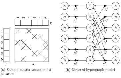
Figure1ashows the sparse matrix and vectors of the SpMxV operation y ← Ax in a sample of the iterative solver application mentioned above. Figure1b
shows the associated directed hypergraph model in the case where a rowwise partitioning is required. In the model, there are three types of vertices (xi, yi,
and ri for i = 1, . . . , 6), each modeling an x- or a y-vector entry, or a row of
A. The vertices are shown as labeled white circles. The nets are shown as filled, small circles. The directions of the pins are set from x-vertices to the corresponding nets, from those nets to the row vertices. The y-vertices are the destinations of the corresponding nets whose sources are the corresponding row vertices.
In the directed hypergraph model of Figure1b, there is a single sender and multiple receivers for each net. This model fits well with many scientific ap-plications where there is a single owner of the data, who is also responsible for distributing the updated value to processors that needs it. There are ap-plications in which there are multiple senders that send, usually, their partial updates to the owner of the data. Some other applications use both of these models iteratively, such as gathering of partial updates followed by distribution of the updated values (e.g., [33]). A directed hypergraph can model such ap-plications. However, the current implementation of UMPa supports only the discussed applications with a single sender. We note that in SpMxV when the partitioning is columnwise or on nonzero basis (that is a two dimensional parti-tioning on the matrix), some nets of the directed hypergraph will have multiple senders, in which case UMPa cannot be used in its current form.
In our directed hypergraph model, a part p corresponds to a processing unit p, and the balance restriction of the partitioning problem on the part weights necessitates a balanced distribution of the computational load among the processing units. In addition, the total communication volume corresponds to the connectivity-1 metric in (2.2).
A 1 2 3 5 6 4 1 2 3 5 6 x y 4
(a) Sample matrix-vector multi-plication 1 r2 r3 r4 r5 r6 y1 y2 y3 y4 y5 y6 x1 x2 x3 x4 x5 x6 ny1 n y 2 n y 3 ny4 ny5 n y 6 n6 x 1 nx 2 nx 3 n x 4 nx 5 n x r
(b) Directed hypergraph model
Figure 1: Sample sparse matrix-vector multiplication and the corresponding directed hyper-graph model.
3.2. Communication cost metrics using direction information
Given a K-way partition, let SV[p] and RV[p] be the data volume the pro-cessing unit p sends and receives, respectively. That is
SV[p] = X part[src[n]]=p c[n](λn− 1) , (3.1) RV[p] = X part[src[n]]6=p p∈prts[n] c[n] . (3.2) Hence, TV equalsPK i=1SV[pi] =P K i=1RV[pi]. Let SRV[p] = SV[p] + RV[p] be
the total volume of data sent/received by the processor p. The maximum data volume sent MSV and sent/received MSRV by a single processor are defined as
MSV = max
i {SV[pi]} , (3.3)
MSRV = max
i {SRV[pi]} . (3.4)
Let SM[pi] be the number of messages the processing unit pi sends, that is
SM[pi] = |{pj: ∃n s.t. part[src[n]] = pi and pj∈ prts[n] \ {pi}}| . (3.5)
The total number of messages TM, and the maximum number of messages sent by a single processor MSM are defined as
TM =X
i
SM[pi] , (3.6)
MSM = max
1
v
4v
3v
6v
2v
5 1n
x 2n
x 3n
x 4n
x 6n
xP
1P
2P
3v
Figure 2: A 3-way partition of the simplified directed hypergraph. A vertex vinow represents
xi, yiand row ri. Among the nets, only the ones that are cut are shown.
Consider again the sparse matrix-vector multiplication of Fig.1 in the con-text of an iterative solver where the vectors x and y undergo linear operations (such as xi ← xi + βyi for a scalar β to form the x of the next iteration).
In this case, the hypergraph can be simplified by using a set of modifications which are useful to avoid some extra communications. First, the data items xi
and yi should be in the same part upon partitioning—otherwise an extra data
transfer is required during the vector operations. Second, yi is produced by
ri; unless they are in the same part, an extra communication is required. It is
therefore advisable to combine the vertices xi, yi, and rifor all i (see the vertex
amalgamation operation introduced in [7]; see also [23]). This simplified model corresponds to the column-net hypergraph model [2]. Consider the 3-way parti-tion of the resulting hypergraph depicted in Fig.2(internal nets are not shown for clarity). Under this partition, the processor p1, corresponding to the part
P1, holds vector entries x1, x4, rows r1, r4 and is responsible for computing y1
and y4at the end of multiplication. Similar data and computation assignments
apply to the processors p2 and p3 corresponding to the parts P2 and P3. As
seen with the directions on the pins of the cut nets, processor p1sends x1to p3
and x4to p2; processor p2 sends x2 to p1 and p3; and p3sends x3and x6 to p1.
Combining these, we see that SV[pi] = 2, for all i; RV[p1] = 3, RV[p2] = 1, and
RV[p3] = 2. We further note that SM[p1] = SM[p2] = 2, SM[p3] = 1.
The directions on the hyperedges help to quantify the sends and receives of each processor. Without directions, one would not know, for example, if the information flow on n3
xshould have been as described. If there were no vertex
amalgamation, it would be possible to compute these without directions, but with a little bookkeeping and additional computation. However, vertex amalga-mation type operations (e.g., the coarsening phase in a multi-level partitioner) always take place in the state-of-the-art partitioners. In this case, quantifying
the sends and receives of each processor would require too much bookkeeping (the contents of a composite vertex and connections of the composing vertices to the nets) and too much computation to be useful in the multi-level partitioning framework. The directions in the nets avoid this difficulty, but necessitate the development of suitable partitioning tools.
4. UMPa: A multi-objective partitioning tool for communication min-imization
The proposed partitioner, UMPa, aims to optimize a given volume- or latency-based primary metric and tries to reduce a set of secondary communication metrics. Although the recursive bisection approach can work well for the total communication volume metric (TV), it is not suitable for the maximum vol-ume (MSV), the total number of messages (TM), and the maximum number of messages sent by a processor (MSM). Since we aim to handle multiple com-munication metrics all together, UMPa follows the direct K-way partitioning approach.
4.1. Multi-level coarsening phase
In this phase, the original hypergraph is gradually coarsened in multiple levels by clustering subsets of vertices at each level. There are two types of clustering algorithms: matching-based and agglomerative. The matching-based algorithms put at most two similar vertices in a cluster, whereas the agglom-erative ones allow any number of similar vertices. There are various similarity metrics—see for example [10, 34, 12]. All these metrics are defined only on two adjacent vertices (one of them can be a vertex cluster). Two vertices are adjacent if they share a net and they can be in the same cluster if they are adjacent.
We use an agglomerative algorithm and the absorption clustering metric using pins [10,34]. For this metric, the similarity between two adjacent vertices u and v is
X
n∈nets[u]∩nets[v]
c[n] |pins[n]| − 1
This is also the default metric in PaToH [10]. In each level `, we start with a finer hypergraph H` and obtain a coarser one H`+1. If VC ⊂ V` is a subset of
vertices deemed to be clustered, we create the cluster vertex u ∈ V`+1 where nets[u] = ∪v∈VCnets[v]. We also update the pin sets of the nets in nets[u]
accordingly.
Since we need the direction, we always store the source vertex of a net n ∈ N as the first pin in pins[n]. To maintain this information, when a cluster vertex u is formed in the coarsening phase, we put u to the head of pins[n] for each net n whose source vertex is in the cluster. We also discard the nets that become singleton at each step of the coarsening phase as well as the initial singleton nets, since they do not cause any communication.
4.2. Initial partitioning phase
To obtain an initial partition for the coarsest hypergraph, we use PaToH [10], which is proved to produce high quality partitions with respect to the total communication volume [2]. We execute PaToH five times and get the best partition according to the given primary metric. We chose to use PaToH for three reasons. First, since we always take TV into account either as a primary or a secondary metric, it is better to start with an initial partition having a good total communication volume. Second, since TV is the sum of the send volumes of all parts, minimizing it should also be good for both MSV and MSRV and even for the latency-based metrics. We verified the second reason, although it sounds intuitive, in preliminary experiments [9]. The third reason is more esoteric. The coarsest hypergraph which has small net sizes and high vertex degrees lends itself gracefully to the recursive bisection and FM-based improvement heuristics (see also elsewhere [18]).
4.3. Uncoarsening phase and one-phase K-way refinement
The uncoarsening phase is realized in multiple levels corresponding to the coarsening levels where at the `th level, we project the partition Π`+1 obtained for H`+1 to H`. Then, we refine it by using a novel K-way refinement heuristic which takes the primary and the secondary metrics into account. The proposed heuristic runs in multiple passes where in a pass it visits each boundary vertex u and either leaves it in part[u], or moves it to another part according to some move selection policy.
UMPa provides refinement methods for four primary metrics: the total com-munication volume TV; the maximum send volume MSV; the total number of messages TM; and the maximum number of messages a processing unit sends MSM. We use the notation UMPaX to denote the partitioner with the primary
objective function X during the refinement. These methods take secondary and sometimes tertiary metrics into accounts. As an aid to the refinement process, the part weights can be used for tie-breaking purposes while selecting the best move.
Since each metric is different, the implementation details of the refinement heuristics are also different. However, their main logic is the same. The heuris-tics perform a number of passes on the boundary vertices. To be precise, UMPa uses at most 2` passes for H`, the hypergraph at the `th coarsening level. We
observed that most of the improvement on the metrics are coming from the refinement on the coarser hypergraphs. Furthermore, since these hypergraphs are smaller, the passes on them take much less time. That is, the impact of these passes are high and their overhead is low. Hence, we decided to perform more passes on the coarser hypergraphs. UMPa also stops the passes when the improvement on the primary metric is not significant during a pass.
The high-level structure of a pass is given in Algorithm 1. In a pass, the heuristic visits the boundaryvertices in a random order and for each visited vertex u and for all p 6= part[u], it computes how the communication metrics in (M1, M2, M3) are affected when u is moved from part[u] to p. This computation
Algorithm 1: A generic pass for K-way refinement
Data: H = (V, N ), (M1, M2, M3): the metrics,
part: the part assignments, W: part weights for each u ∈ boundary do
pbest←part [u]
1 Lbest← (gainM1, gainM2, gainM3) ← leaveVertex(H, u, part)
2 for each part p 6= part[u] do
if p has enough space for vertex u then
3 L = (lossM1, lossM2, lossM3) ← putVertex (H, u, p)
4 (pbest, Lbest) ← selectMove(p, L, pbest, Lbest, W )
if pbest6= part[u] then
5 move u to pbest,
update part, W and the other data structures accordingly
is realized in two steps. First, u is removed from part[u] and the leave gains for the communication metrics are computed with leaveVertex (line1). Second, u is tentatively put into a candidate part p and the arrival losses are calculated with putVertex (line3). We first set the processing unit for the best move as pbest= part[u]. Since the leave gains and arrival losses are equal while removing
a vertex from its part and putting it back (the total gain is zero), initially, the best arrival loss triplet Lbest is set to (gainM1, gainM2, gainM3). Then, for each
possible target processing unit p, the arrival losses on the metrics are computed. With the selectMove heuristic, which is given in Algorithm 2, these losses are compared with Lbestto select the best move (line4). After trying all target
processing units and computing the arrival losses of the corresponding moves, u is moved to pbest. If pbest6= part[u] the data structures, such as boundary, part, λ,
and Λ, used throughout the partitioning process are updated accordingly. Algorithm 2: The generic selectMove operation
Data: p, L = (L1, L2, L3), p0, L0= (L01, L 0 2, L 0 3), W if L1< L01 then
return (p, L) .Primary metric
else if L1= L01 and L2< L02 then
return (p, L) .Secondary metric
else if L1= L01, L2= L02 and L3< L03 then
return (p, L) .Tertiary metric
else if L1= L01, L2= L02, L3= L03 and Wp< Wp0 then
return (p, L) .Tie-breaking
return (p0, L0)
The selectMove heuristic given in Algorithm 2 compares two vectors (L1, L2, L3, Wp) and (L10, L02, L03, Wp0). Starting from the first ones, it compares
the vector entries one by one. When a smaller entry is found, the corresponding processing unit is returned as the better candidate.
5. Multi-objective one-phase K-way Refinement
Although the structure of a pass and the execution logic is the same, the computation of the leave gains and arrival losses differ with respect to the com-munication metrics used. Here we describe the implementation of the functions leaveVertex and putVertex for UMPaTV, UMPaMSV with secondary and
tertiary metrics MSRV and TV, and UMPaTM with a secondary metric TV. We
also implemented UMPaMSMand used it in the experiments. But we do not give
the details of its leave gain and arrival loss computations since the structure of these algorithms is similar to the ones described below.
5.1. Total communication volume
In the directed hypergraph model, the total volume of the communica-tion sent/received throughout the execucommunica-tion corresponds to the cutsize defi-nition (2.2) as in the standard hypergraph model. In other words, the TV metric is global and hence, the sense of direction does not have any effect in its computation. Here we describe UMPaTV which takes a single communication
metric TV into account, i.e., it is a standard hypergraph partitioner with the traditional objective function (2.2).
Algorithm 3: leaveVertexTV
Data: H = (V, N ), u, part
gainTV← 0
Pu← ∅
for each n ∈ nets[u] do if Λ(n, part[u]) = 1 then
1 gainTV← gainTV+ c[n]
2 Pu← Pu∪ prts[n]
return(gainTV, Pu)
As described above, the refinement heuristic performs passes on the bound-ary vertices. Let u be the boundbound-ary vertex visited during a pass. The leaveV-ertexTV method given in Algorithm3computes the gain on TV when u leaves part[u]. After the move, there will be a gain if and only if the target proces-sor p contains at least one vertex which shares a net with u. Let Pu be the
set of such parts. To be more efficient, this set can be computed beforehand and the for loop in Algorithm1 (line 2) can be iterated over p ∈ Pu instead
of p ∈ {1, . . . , K} \ part[u]. For this reason, leaveVertexTV also builds this set (line2) while computing gainTV.
After u leaves part[u] and the leave gain is computed, the refinement heuristic computes the arrival losses for all target parts Pu\part[u]. Algorithm4gives the
description of the putVertexTV function. Given u and a part p, the function computes the increase on TV after putting u to p. For each net n ∈ nets[u], TV increases by c[n] if u will be the only pin of n in p (line1).
Algorithm 4: putVertexTV
Data: H = (V, N ), u, p (the candidate part)
lossTV← 0
for each n ∈ nets[u] do if Λ(n, p) = 0 then
1 lossTV← lossTV+ c[n]
return lossTV
5.1.1. Total number of messages
Although the directionality is not important for the total volume, the flow of communication is crucial while minimizing other metrics. Hence for each net n affected by a move, we need to use the source information src[n]. Here we describe the leave gain and arrival loss computations of UMPaTM which
minimizes the total number of messages throughout the execution by also taking the total volume of communication, TV, into account as the secondary metric.
Let netComm(p, p0) be the number of nets n such that p, p0 ∈ prts[n] and src[n] = p, i.e., the number of data to be sent from the processing unit p to the processing unit p0. The refinement heuristic performs passes on the boundary vertices. Let u be the boundary vertex visited during a pass. When u leaves part[u], the gains on TM and TV are computed by leaveVertexTM given in Algorithm5. The gain on TV (line1) is computed as described in the previous subsection. For the gain on TM, there are two cases:
1. u is the source pin of a net n (line2): For each part p ∈ prts[n], there is a gain if netComm(part[u], p) = 0 after removing u from part[u]. Note that a vertex can be a source for multiple nets.
2. u is a non-source pin of a net n (line4): Let psender be the part having
the source of n. There is a gain if netComm(psender, part[u]) = 0 after
removing u from part[u].
In addition to gain computations, the set of the parts that receive data from u (i.e., u is the source of a net connected to the receiver part), receivers, and send data to u (i.e., u is a non-source pin of a net whose source is in the sender part), senders, are obtained. These sets are used to efficiently compute the arrival losses for each target part candidate.
After the leave gains are computed with leaveVertexTM, the heuristic tentatively moves the boundary vertex to the candidate parts and computes the losses on the communication metrics with putVertexTM given in Algorithm6. Let p be the target part. The function first computes the arrival loss on TV as described in the previous subsection. Then for all preceiver ∈ receivers, it
checks if a new message from p to preceiver is necessary. This implies a loss
on TM. It repeats a similar process for all psender ∈ senders and checks if a
message from psender to p, which was not necessary before the move, is now
Algorithm 5: leaveVertexTM
Data: H = (V, N ), u, part
gainTV← 0, gainTM← 0
senders ← ∅, receivers ← ∅
pu← part[u]
for each n ∈ nets[u] do
1 if Λ(n, pu) = 1 then gainTV← gainTV+ c[n] 2 if src[n] = u then if Λ(n, pu) > 1 then receivers ← receivers ∪ {pu} 3 for each p ∈ prts[n] \{pu} do receivers ← receivers ∪ {p} netComm(pu, p) ← netComm(pu, p) − 1 if netComm(pu, p) = 0 then gainTM← gainTM+ 1 4 else psender← part[src[n]]
senders ← senders ∪ {psender}
if Λ(n, pu) = 1 then
netComm(psender, pu) ← netComm(psender, pu) − 1
if netComm(psender, pu) = 0 then
gainTM← gainTM+ 1
return (gainTM, gainTV, senders, receivers)
Algorithm 6: putVertexTM
Data: H = (V, N ), u, p (the candidate part), senders, receivers
lossTM← 0, lossTV← 0
for each n ∈ nets[u] do if Λ(n, p) = 0 then
lossTV← lossTV+ c[n]
1 for each preceiver∈ receivers do
if netComm(p, preceiver) = 0 then
lossTM← lossTM+ 1
2 for each psender∈ senders do
if netComm(psender, p) = 0 then
lossTM← lossTM+ 1
5.1.2. Maximum communication volume
Here we describe UMPaMSV which minimizes MSV, the maximum volume
sent by a processing unit, and also takes MSRV (the maximum send and receive volume), and TV into account as the secondary and tertiary metrics, respec-tively. This metric configuration is useful when one wants a partition which does not yield a bottleneck processor and does not use the network extensively. The generic structure of the refinement heuristic given in Algorithm1 also applies to the local communication metrics such as MSV and MSM. But for an efficient implementation, we slightly alter this structure for UMPaMSV. When
a vertex is taken from its part and put to another one during the refinement, instead of computing the exact gains/losses on the metrics, we compute a set of intermediate values which correspond to the changes in the send/receive volumes of a processing unit p, i.e., SV[p] and RV[p]. After each move, these intermediate values are used to compute the exact changes on the metrics, and the best move is selected in a similar fashion.
Algorithm 7: leaveVertexMSV
Data: H = (V, N ), u, part toOldP art ← 0
gainRV ← 0
for each processing unit p do
gainSV[p] ← 0
pu← part[u]
for each n ∈ nets[u] do psender← part[src[n]] if src[n] = u then
gainSV[pu] ← gainSV[pu] + c[n](λn− 1)
1 if Λ(n, pu) > 1 then
gainRV ← gainRV − c[n]
toOldP art ← toOldP art + c[n] else
if Λ(n, pu) = 1 then
2 gainSV[psender] ← gainSV[psender] + c[n]
3 gainRV ← gainRV + c[n]
return (gainSV, gainRV, toOldP art)
Algorithm7describes the leaveVertexMSV function. To store the changes
on the send volumes of the processing units after the leave operation, the func-tion uses an array gainSV[·] of size K. It also stores the change on RV[part[u]],
i.e., the receive volume of part[u], in a variable gainRV. If u is the source for a
net n, removing u yields c[n](λn− 1) gain on the send volume of part[u]. But
after the move, there will also be an increase on RV[part[u]] if there are more pins of n in part[u] (line1). The potential increase due to the nets having u as the source does not depend on the target part. It is stored in a variable
toOldP art which later will be used by the putVertexMSV function to com-pute the overall change on the send volume of each target part. When u leaves part[u], RV[part[u]] decreases by c[n] if u is not the source of n and if it is the only pin of n in part[u] (line2). The same decrease must also be observed on
SV[psender], the send volume of the part containing u’s source pin (line3).
If u is the source pin of n, as described above, we take the gain on SV[part[u]] into account. However, we do not do the same for the corresponding gains on the RV values of other parts in prts[n]. That is, we do not compute all the reductions on RV, and hence, if we compute the metrics here the MSRV value will not be exact. Although exact RV values and hence the exact gains on the metrics can be computed, we chose to follow this approach to be more efficient. Because, after putting u to the target part p, these reductions on the receive volumes of the processing units in prts[n] \{part[u], p} will not be effective anymore since these processing units will continue to receive n’s data from p. Hence, if one computes the exact RV values here most of the computation will be redundant. The details of the putVertexMSV function are given in Algorithm8. Sim-ilar to leaveVertexMSV, the algorithm computes the increase on the send volumes of all parts and the increase on the receive volume of the target part p. After the move, the target processing unit will send the data which was sent by part[u] before. Hence, the value lossSV[p] must cover gainSV[pu]. It also needs
to contain the amount of the communication from p to part[u] due to the nets having u as the source that remain connected to part[u], i.e., toOldP art (line1). The rest of the loss updates are similar to the ones in the previous algorithms.
Algorithm 8: putVertexMSV
Data: H = (V, N ), u, p (the candidate part), gainSV, toOldP art, part
lossRV ← 0
for each processing unit q do
lossSV[q] ← 0
pu← part[u]
1 lossSV[p] ← gainSV[pu] + toOldP art
for each n ∈ nets[u] do psender← part[src[n]] if src[n] = u then if Λ(n, p) > 0 then 2 lossSV[p] ← lossSV[p] − c[n] lossRV ← lossRV − c[n] else if Λ(n, p) = 0 then
lossSV[psender] ← lossSV[psender] + c[n]
lossRV ← lossRV + c[n]
return (lossSV, lossRV)
Firstly, u is removed from part[u], and the intermediate values, partial gains on the send/receive volumes, are computed by leaveVertexMSV. Then, u is tentatively put to each target candidate p, and the intermediate values, arrival losses on the send/receive volumes, are obtained by putVertexMSV. As de-scribed above, although these intermediate values are inexact, their sum gives the exact change on the send/receive volumes for each processor. After com-puting these changes and the send/receive volumes after the move, the metrics are computed and the best move is selected in a similar fashion. That is the move with the smallest value on the primary metric is preferred. If these values are equal for two target processors, then the secondary metric is considered. In case of equality for the secondary metric values, the tertiary metric is taken into account. As we will show in the experimental results section, this move selection policy and tie-breaking scheme have positive impact on all the communication metrics.
Algorithm 9: A pass for K-way maximum send volume refinement
Data: H = (V, N ), part: the part assignments, W: part weights for each u ∈ boundary do
(gainSV, gainRV, toOldP art) ← leaveVertexMSV(H = (V, N ), u, part)
Mbest← (M SV, M SRV, T V )
pbest← part[u]
for each part p 6= part[u] do
if p has enough space for vertex u then
(lossSV, lossRV) ← putVertexMSV(H, u, p, gainSV,
toOldP art, part)
1 for each part q do
∆S← lossSV[q] − gainSV[q]
SV0[q] ← SV[q] + ∆S
SRV0[q] ← SV[q] + ∆S+ RV[q]
SRV0[part[u]] ← SRV0[part[u]] − gainRV
SRV0[p] ← SRV0[p] + lossRV
Mp← (max(SV0), max(SRV0), T V + lossRV − gainRV)
(pbest, Mbest) ← selectMoveMSV(p, M, pbest, Mbest, W )
if pbest6= part[u] then
move u to pbest,
update part, W and the other data structures accordingly
5.1.3. Implementation Details
During the gain computations, the heuristic uses the connectivity informa-tion between the nets and parts stored in data structures λ, Λ, and netComm. These structures are constructed after the initial partitioning phase and main-tained by the uncoarsening phase. When a vertex u is moved, we revisit the nets of u and update the data structures accordingly. When new boundary vertices are detected, they are inserted to the array boundary and visited in the same pass. We restrict the number of moves for a vertex u during a pass to 4, in order to limit the execution time. When this number is reached the vertex is
locked and removed from the boundary. Let ρ =P
n∈N|pins[n]| be the number of pins in a hypergraph. For UMPaTV,
considering the restriction on the number of moves per vertex, the time com-plexity of the leave gain and arrival loss computations is O(ρ) and O(ρK), respectively. Hence, the overall complexity of a refinement pass is O(ρK). The factor K comes from the number of candidate target parts for each move. For UMPaTV, we only visit the boundary vertices and try the parts of the visited
vertex’s nets as target candidates. In practice, these numbers are much smaller than |V| and K as a side-effect of the minimization of the objective functions.
For UMPaTM, UMPaMSV, and UMPaMSM, the overall time complexity of a
refinement pass is O(ρK + |V|K2) since all these variants need an additional
for loop which iterates O(K) times (lines1 and2 in Algorithm6and line1 in Algorithm9). However, since only the boundary vertices and parts of the nets are visited, the factors are much smaller in practice, and the worst-case analysis is very loose.
To store the numbers of pins per part for each net, Λ, we use a 2-dimensional array. Hence, the space complexity is O(K|N |). This can be improved by using a sparse storage as shown in [18].
6. Experimental results
The experiments are conducted on a computer with 2.27GHz dual quad-core Intel Xeon CPUs and 48GB main memory.
We compare the quality and efficiency of the partitioners UMPa, Zoltan [12], Mondriaan [11] (version 4.0) and PaToH [10] (in default setting)1. UMPa is implemented in C++, while the other partitioners are implemented in C. All im-plementations are compiled with the gcc suite version 4.4.4. To obtain our data set, we used several graphs with 100K–1, 500K vertices and 409K–38, 354K edges from the 10th DIMACS implementation challenge dataset [35] which contains 38 graphs from eight different classes. The names and the details of these graphs are given in Table 1. These graphs are translated into hypergraphs using the column-net model to fit the problem definition of the 10th DIMACS challenge2.
In all of our experiments, the vertices have unit weights, while the nets may have non-uniform costs (as in the ComputationalTask graphs). Although Zoltan hy-pergraph partitioner is designed to work on distributed memory machines, all executions are run serially in our experiments. The reported results are the averages of five different executions. The performances of the partitioners are evaluated for five different communication metrics in addition to execution time. These are the maximum send volume (MSV), the maximum send/receive vol-ume (MSRV), the total volvol-ume (TV), the maximum send message (MSM), and
1The default setting of PaToH is chosen instead of quality setting, as the quality option
obtains only 4% better cut sizes. On the other hand, the default option is 3.56 times faster.
the total message (TM). The chosen hypergraphs are partitioned into 128, 256, 512, and 1024 parts with ε=0.03.
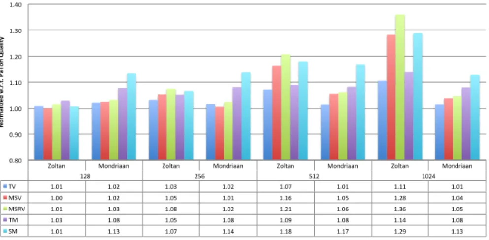
We first compare the execution time and the quality of the existing hyper-graph partitioning tools. Although Mondriaan uses a hyperhyper-graph model, the partitioner is specifically designed for matrices, and it does not accept non-uniform net weights. For this reason, the experiment is run on 36 (out of 38) graphs excluding the ones in the ComputationalTask class. We adjust Mondri-aan as described in [36] for the experiment. Figure3 gives the communication metrics and execution times of Zoltan and Mondriaan normalized w.r.t. PaToH. As seen in the figure, Mondriaan obtains partitions whose TV values are similar to that of PaToH on TV. However, its quality on the other metrics is slightly worse. Furthermore, it is significantly slower than PaToH. Although the par-titions found by Zoltan yield similar communication metrics when K is small, Zoltan’s partitioning quality gets worse as K increases. We attribute this to the simplified refinement implementations for the parallelization purposes. Since PaToH obtains the best quality and the best serial execution time, we compare the performance of UMPa against PaToH for the rest of the experiments. A fair comparision between UMPa and existing work [7,8] is not feasible due to the different partitioning contexts, as noted before (in Sections2.4and3.1).
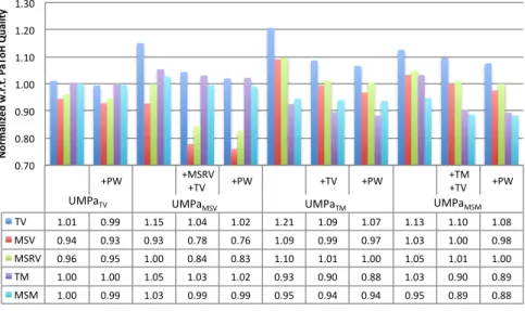
Figures 4 and 5 show the average values of the metrics normalized with respect to the corresponding average metric value of PaToH partition. Each column of the table (and its visual representation as a group of five bars) cor-responds to an UMPa variant with a different metric and tie-breaking combi-nation, while each row of the table corresponds to the values with respect to a different communication metric. We experimented with four main variants UMPaX with the primary metric X ∈ {TV, MSV, TM, MSM}. For each of these
variants, we tried different combinations where in the first one only the primary metric is taken into account with no tie-breaking. Then, except for UMPaTV,
we obtained a variant which use additional metrics (shown with a ‘+’ sign in the figures). At last, we added tie-breaking and obtained the full variant (shown with “+ PW” in the figures). We executed each of these 11 variants and Pa-ToH on all 38 hypergraphs 5 times and obtain 5 different partitions. For each variant/metric pair, the geometric mean of these 190 executions are computed, and the averages for the UMPa variants are normalized with respect to PaToH’s averages. The figures show these normalized values.
As the first two columns in the tables (and the first two bar groups) of the figures show, for various K values, UMPaTV is as good as PaToH for all
the communication metrics. Furthermore, its MSV and MSRV (2nd and 3rd rows/bars) values are 4-8% better than PaToH for all K values. The tie-breaking scheme (the second column denoted with PW), which uses the part weight in-formation, improves the performance of UMPaTV (the first column) by around
2%. Since the direction information is not important while minimizing TV, the undirected hypergraph model and recursive bisection can be used as is. There-fore, the proposed directed hypergraph model and the K-way partitioning do not have an advantage for TV unlike for the other communication metrics as we discuss below.
Zoltan Mondriaan Zoltan Mondriaan Zoltan Mondriaan Zoltan Mondriaan 128 256 512 1024 TV 1.01 1.02 1.03 1.02 1.07 1.01 1.11 1.01 MSV 1.00 1.02 1.05 1.01 1.16 1.05 1.28 1.04 MSRV 1.01 1.03 1.08 1.02 1.21 1.06 1.36 1.05 TM 1.03 1.08 1.05 1.08 1.09 1.08 1.14 1.08 SM 1.01 1.13 1.07 1.14 1.18 1.17 1.29 1.13 0.80 0.90 1.00 1.10 1.20 1.30 1.40 N or m al iz ed w .r .t . P aT oH Qu al ity
(a) Normalized communication metrics
128 256 512 1024 Zoltan 1.63 1.67 1.71 1.74 Mondriaan 3.87 3.83 3.87 3.91 0.00 0.50 1.00 1.50 2.00 2.50 3.00 3.50 4.00 Nor m aliz ed w.r .t. P aToH Tim e
(b) Normalized execution times
Figure 3: The normalized communication metrics and execution times of Zoltan and Mondri-aan w.r.t. PaToH for K ∈ {128, 256, 512, 1024}.
We experimented with three UMPaMSV variants to carefully evaluate the
ef-fects of the secondary and tertiary objectives and the tie-breaking mechanism. Although minimizing only with the primary metric and no tie-breaking (col-umn 3) obtains 7–11% better MSV value, with respect to the other metrics, UMPaMSV is worse than PaToH. Using MSRV and TV as the secondary and
tertiary objectives (column 4) has positive effects on the other communication metrics. Moreover, this approach further improves the primary communication metric MSV. This variant of UMPaMSV doubles the improvement on the
pri-mary metric MSV and reduces it 17–22% on the average. Furthermore, it also obtains decent values for the other metrics with respect to PaToH. Extending the refinement with part weight tie-breaking (column 5) also reduces all the volume-based communication metrics around 2%. These observations are not only true on the average but also for most of the graphs in the dataset. For all partitionings with different K values, UMPaMSV with tie-breaking obtains more
and 20% for 13 graphs, and between 2% to 10% for the remaining 13 graphs. Only with a primary metric, UMPaTM with no tie-breaking (column 6)
im-proves TM about 7–12%. It also imim-proves MSM with respect to PaToH, but its effect is almost always negative for the volume-based metrics. Using TV as the secondary objective to UMPaTM (column 7) reduces the increase on these
met-rics. Furthermore, it also improves TM by 2–3% more. Similar to other cases, the communication metrics are improved around 3% more with the addition of tie-breaking (column 8).
The results for UMPaMSMare similar to that of other variants. Only with the
primary objective function (column 9), UMPaMSM obtains 5–7% better MSM
values than PaToH. Using TM and TV as the secondary and tertiary objec-tives (column 10) makes the difference around 7–19%. A further 2–3% improve-ment is obtained with the addition of tie-breaking (column 11).
Figure6shows the UMPa variants’ runtimes normalized with respect to Pa-ToH. As a K-way partitioner, the complexity of the refinement is linear with the number of parts for UMPaTV and UMPaTM, and quadratic for UMPaMSV and
UMPaMSM. Therefore, as K increases, the proposed direct K-way method is
ex-pected to be slower than a recursive-bisection-based partitioner. For 128 parts, except UMPaMSV, the execution times are closer to that of PaToH. However,
when the number of parts get bigger, the slowdown increases.
Table 1 gives the individual execution times and the volume metric results of PaToH for K = 512. The normalized execution times and normalized volume metrics of the UMPa variants are listed on the right side of the table. As seen in the table, the best TV improvement of the UMPaTVis 18% improvement on
G n pin pout, while it obtains 5% TV degrade on eu-2005. UMPaMSV obtains
its best MSV improvement on preferentialAttachment as 85%, while it obtains its worst improvement on thermal2 graph by 1%. UMPaTMand UMPaMSMhave
their best improvements on smallworld as 45% and 43%, respectively.
As Table1 shows, the Citation and Clustering graphs have relatively large MSV, TM, and MSM values compared to other classes. For these graphs, the UMPa variants obtain decent improvements. However, when these metrics have small values, e.g., PaToH’s MSM values for the Sparse class, the improvements are not significant. Since PaToH minimizes only the total communication vol-ume, a small metric value implies that minimizing TV also minimizes that met-ric. We believe that this is due to the structure of the graphs. For example, the Delaunay graphs are planar. Hence, when PaToH puts similar vertices in the same part, the nets connected to a part will have similar pin sets. Even if some of these nets are in the cut, the corresponding communications can be packed into a few messages. The same argument is also true for the Random Geometric graphs where only the vertices close to each other in the Euclidian space are connected.
7. Conclusions and future work
We proposed a directed hypergraph model and a multi-level partitioner UMPa. The partitioner uses a novel K-way refinement heuristic employing
T able 1 : The exp erimen t results for K = 512. The actual execution time (TT ) and the v olume metrics of P aT oH are giv en on the left side of the table. The normalize d time and nor m a lized primary v olume metrics of UMP a v ar ia n ts (with full tie-breaking sc heme) are giv en on the righ t side of the table. P aT oH UMP aTV UMP aMSV UMP aTM UMP aMSM Graph Class V ertices Edges TT TV MSV TM MSM TT TV TT MSV TT TM TT MSM citationCiteseer Citation 268,495 1,156,647 24.17 449,324 3,230 53,824 252 3.30 0.95 6.64 0.62 4.11 0.64 6.50 0.58 coAuthorsCiteseer Citation 227,320 814,134 7.23 128,873 1,147 41,486 190 2.35 0.97 7.17 0.60 3.91 0.63 6.64 0.63 coAuthorsDBLP Citation 299,067 977,676 10.87 274,463 2,524 78,531 300 3.07 0.97 8.72 0.59 4.98 0.61 7.84 0.67 coP ap ersCiteseer Citation 434,102 16,036,720 249.29 656,097 5,100 53,467 198 0.22 0.95 1.56 0.77 0.36 0.69 1.12 0.74 coP ap ersDBLP Citation 540,486 15,245,729 157.64 1,592,718 9,388 106,073 334 0.70 0.90 3.40 0.77 1.03 0.71 2.42 0.81 caidaRouterLev el Clustering 192,244 609,066 8.39 132,375 4,886 20,491 384 2.81 0.98 6.93 0.60 3.78 0.74 6.16 0.61 cnr-2000 Clustering 325,557 2,738,969 28.14 288,308 4,241 6,411 154 3.26 0.95 6.93 0.73 3.90 0.75 5.73 0.78 eu-2005 Clustering 862,664 16,138,468 215.40 1,568,558 11,704 22,600 251 2.81 1.05 6.68 0.73 3.09 0.68 5.22 0.70 G n pin p out Clustering 100,000 501,198 12.15 719,743 1,584 230,910 480 5.20 0.82 7.01 0.81 6.32 0.62 9.14 0.71 in-2004 Clustering 1,382,908 13,591,473 160.83 449,886 7,297 10,898 182 1.08 1.01 2.83 0.68 1.46 0.59 2.74 0.66 preferen tialA ttac hmen t Clustering 100,000 499,985 16.91 755,796 26,256 190,519 511 5.77 0.97 8.48 0.15 6.34 0.67 6.29 1.00 smallw orld Clustering 100,000 499,998 5.29 235,807 558 137,196 302 5.02 0.96 7.84 0.89 6.73 0.55 11.82 0.57 1,280,000 ComputationalT ask 1,279,253 1,285,172 14.72 2,194,852,000 69,956,800 3,033 47 2.59 1.01 2.57 0.90 2.65 0.57 2.59 0.90 320,000 ComputationalT ask 320,142 322,473 9.30 1,066,920,000 50,649,680 2,481 51 1.58 1.02 2.15 0.56 2.01 0.72 2.09 0.57 delauna y n17 Delauna y 131,072 393,176 3.50 29,990 81 3,028 10 2.98 1.01 6.05 0.95 3.37 1.00 4.27 0.98 delauna y n18 Delauna y 262,144 786,396 6.28 41,748 112 3,032 12 2.89 1.01 5.15 0.96 3.42 1.00 4.14 0.89 delauna y n19 Delauna y 524,288 1,572,823 11.24 58,493 165 3,035 11 1.50 1.01 4.38 0.89 2.11 1.00 2.82 0.85 delauna y n20 Delauna y 1,048,576 3,145,686 20.60 82,067 213 3,026 10 1.36 1.01 3.49 0.98 1.99 1.00 2.50 0.94 rgg n 2 17 s0 RandomGeometric 131,072 728,753 4.26 29,206 96 2,864 12 2.08 1.00 5.70 0.89 2.70 0.91 3.21 0.83 rgg n 2 18 s0 RandomGeometric 262,144 1,547,283 8.37 43,052 132 2,885 11 1.70 0.99 4.06 0.93 2.26 0.92 2.65 0.91 rgg n 2 19 s0 RandomGeometric 524,288 3,269,766 16.95 63,291 193 2,898 11 1.56 1.00 3.51 0.89 1.85 0.96 2.31 0.89 rgg n 2 20 s0 RandomGeometric 1,048,576 6,891,620 35.78 94,118 288 2,896 9 0.69 1.00 2.31 0.88 1.04 0.96 1.38 0.98 af shell10 Sparse 1,508,065 25,582,130 103.09 252,404 647 2,886 8 0.32 1.02 1.13 0.96 0.40 1.00 0.73 1.00 af shell9 Sparse 504,855 8,542,010 35.56 144,713 370 2,804 8 0.51 1.00 1.61 0.95 0.60 1.00 1.03 1.00 audikw1 Sparse 943,695 38,354,076 357.19 947,370 2,824 5,284 21 0.27 1.02 1.57 0.94 0.35 0.95 0.75 0.98 ecology1 Sparse 1,000,000 1,998,000 13.50 79,633 207 2,895 9 1.85 1.04 4.58 0.98 2.76 0.99 3.27 0.87 ecology2 Sparse 999,999 1,997,996 13.46 79,373 205 2,895 9 1.86 1.04 4.58 0.98 2.82 0.99 3.24 0.91 G3 circuit Sparse 1,585,478 3,037,674 26.09 147,446 423 2,975 12 1.56 1.02 5.40 0.96 2.28 0.98 2.91 1.02 ldo or Sparse 952,203 22,785,136 121.70 216,259 661 3,008 14 0.25 1.00 1.61 0.88 0.30 1.00 0.62 1.01 thermal2 Sparse 1,227,087 3,676,134 25.88 95,963 250 2,831 9 0.77 1.03 3.12 0.99 1.34 1.00 1.79 1.00 b elgium.osm Street 1,441,295 1,549,970 10.01 12,526 75 3,000 14 1.29 1.02 2.06 0.87 1.59 0.82 1.85 0.68 luxem b ourg.osm Street 114,599 119,666 0.85 3,397 20 2,144 9 3.17 1.01 4.83 0.85 3.82 0.81 4.29 0.74 144 W alsha w 144,649 1,074,393 11.75 128,880 442 5,665 33 2.81 0.99 6.64 0.91 3.20 0.93 4.02 0.88 598a W alsha w 110,971 741,934 8.52 103,693 372 5,514 31 3.27 0.99 6.93 0.88 3.67 0.93 4.32 0.83 auto W alsha w 448,695 3,314,611 34.37 273,173 806 5,598 29 1.89 1.00 6.96 0.89 2.44 0.94 3.16 0.80 fe o cean W alsha w 143,437 409,593 5.51 83,761 247 5,284 19 3.48 1.04 7.36 0.94 4.18 0.90 4.92 0.91 m14b W alsha w 214,765 1,679,018 16.82 158,215 563 5,347 37 2.90 1.00 6.94 0.89 3.39 0.94 4.52 0.85 w a v e W alsha w 156,317 1,059,331 10.94 142,792 421 6,758 37 2.81 1.00 6.87 0.89 3.13 0.92 4.23 0.72 GEOMEAN 19.20 234,643 1,167 7,954 38 1.68 0.99 4.26 0.80 2.18 0.83 3.10 0.81 BEST 0.22 0.82 1.13 0.15 0.30 0.55 0.62 0.57 W ORST 5.77 1.05 8.72 0.99 6.73 1.00 11.82 1.02
+PW +MSRV+TV +PW +TV +PW +TM+TV +PW TV 1.01 0.99 1.15 1.04 1.02 1.21 1.09 1.07 1.13 1.10 1.08 MSV 0.94 0.93 0.93 0.78 0.76 1.09 0.99 0.97 1.03 1.00 0.98 MSRV 0.96 0.95 1.00 0.84 0.83 1.10 1.01 1.00 1.05 1.01 1.00 TM 1.00 1.00 1.05 1.03 1.02 0.93 0.90 0.88 1.03 0.90 0.89 MSM 1.00 0.99 1.03 0.99 0.99 0.95 0.94 0.94 0.95 0.89 0.88 0.70 0.80 0.90 1.00 1.10 1.20 1.30 N or m al iz ed w .r .t . P aT oH Qu al ity
UMPaMSV UMPaTM UMPaMSM
UMPaTV (a) K = 128 +PW +MSRV +TV +PW +TV +PW +TM +TV +PW TV 1.01 0.99 1.10 1.03 1.01 1.18 1.09 1.07 1.09 1.10 1.08 MSV 0.94 0.93 0.93 0.81 0.79 1.08 1.01 0.98 1.01 1.00 0.98 MSRV 0.95 0.94 0.98 0.85 0.83 1.07 1.01 1.01 1.01 1.00 0.99 TM 1.01 1.01 1.05 1.03 1.02 0.90 0.87 0.85 1.04 0.88 0.86 MSM 1.00 1.00 1.00 0.99 0.99 0.93 0.93 0.92 0.94 0.85 0.84 0.70 0.80 0.90 1.00 1.10 1.20 1.30 N or m al iz ed w .r .t . P aT oH Qu al ity
UMPaMSV UMPaTM UMPaMSM
UMPaTV
(b) K = 256
Figure 4: The normalized metrics of UMPa w.r.t. PaToH for K = 128 and K = 256.
a tie-breaking scheme to handle multiple communication metrics. UMPa yields good communication patterns by reducing multiple communication metrics all together.
Although most of the previous research has mainly focused on the minimiza-tion of the total communicaminimiza-tion volume, there are studies on the minimizaminimiza-tion of multiple metrics. Existing hypergraph-based solutions on multiple metrics
fol- +PWfol- +MSRV+TV +PW +TV +PW +TM+TV +PW TV 1.01 0.99 1.08 1.02 1.00 1.17 1.10 1.09 1.07 1.11 1.10 MSV 0.95 0.94 0.93 0.83 0.80 1.08 1.02 1.01 1.00 1.02 1.01 MSRV 0.96 0.95 0.97 0.88 0.85 1.08 1.03 1.04 1.01 1.02 1.03 TM 1.01 1.01 1.04 1.02 1.02 0.88 0.85 0.83 1.03 0.86 0.84 MSM 1.01 1.00 1.01 1.00 1.00 0.91 0.91 0.91 0.94 0.82 0.81 0.70 0.80 0.90 1.00 1.10 1.20 1.30 N or m al iz ed w .r .t . P aT oH Qu al ity UMPaTV UMPa MSV UMPaTM UMPa MSM (a) K = 512 +PW +MSRV+TV +PW +TV +PW +TM+TV +PW TV 1.00 0.99 1.05 1.02 1.00 1.13 1.09 1.08 1.05 1.09 1.09 MSV 0.94 0.92 0.89 0.81 0.79 1.04 1.01 1.00 0.97 0.99 0.98 MSRV 0.96 0.95 0.94 0.86 0.84 1.05 1.02 1.04 0.98 1.01 1.01 TM 1.01 1.01 1.04 1.02 1.02 0.89 0.87 0.85 1.03 0.88 0.86 MSM 0.98 0.97 0.99 0.97 0.97 0.90 0.90 0.90 0.93 0.81 0.80 0.70 0.80 0.90 1.00 1.10 1.20 1.30 N or m al iz ed w .r .t . P aT oH Qu al ity UMPaTV
UMPa MSV UMPa TM UMPa MSM
(b) K = 1024
Figure 5: The normalized metrics of UMPa w.r.t. PaToH for K = 512 and K = 1024.
low a two-phase approach where in each phase a different metric is minimized, sometimes at the expense of others. UMPa follows a one-phase approach where all the communication cost metrics are effectively minimized in a multi-objective setting where reductions in all metrics can be achieved at the same time, thanks to the proposed directed hypergraph model (undirected models were discussed to be inadequate). We conducted experiments with large hypergraphs and up