Publisher’s version / Version de l'éditeur:
Vous avez des questions? Nous pouvons vous aider. Pour communiquer directement avec un auteur, consultez la première page de la revue dans laquelle son article a été publié afin de trouver ses coordonnées. Si vous n’arrivez pas à les repérer, communiquez avec nous à [email protected]. Questions? Contact the NRC Publications Archive team at
[email protected]. If you wish to email the authors directly, please see the first page of the publication for their contact information.
https://publications-cnrc.canada.ca/fra/droits
L’accès à ce site Web et l’utilisation de son contenu sont assujettis aux conditions présentées dans le site LISEZ CES CONDITIONS ATTENTIVEMENT AVANT D’UTILISER CE SITE WEB.
Proceedings of the 11th ACM SIGKDD International Conference onKnowledge
Discovery and Data Mining (KDD 2005) [Proceedings], 2005
READ THESE TERMS AND CONDITIONS CAREFULLY BEFORE USING THIS WEBSITE. https://nrc-publications.canada.ca/eng/copyright
NRC Publications Archive Record / Notice des Archives des publications du CNRC :
https://nrc-publications.canada.ca/eng/view/object/?id=fc7a6465-83c8-44db-b4ad-6edaf6fa383d
https://publications-cnrc.canada.ca/fra/voir/objet/?id=fc7a6465-83c8-44db-b4ad-6edaf6fa383d
NRC Publications Archive
Archives des publications du CNRC
This publication could be one of several versions: author’s original, accepted manuscript or the publisher’s version. / La version de cette publication peut être l’une des suivantes : la version prépublication de l’auteur, la version acceptée du manuscrit ou la version de l’éditeur.
Access and use of this website and the material on it are subject to the Terms and Conditions set forth at
Learning to Predict Train Wheel Failures
National Research Council Canada Institute for Information Technology Conseil national de recherches Canada Institut de technologie de l'information
Learning to Predict Train Wheel Failures *
Yang, C., and Létourneau, S.
August 2005
* published in The Proceedings of the 11th ACM SIGKDD International Conference on
Knowledge Discovery and Data Mining (KDD 2005). Chicago, Illinois, USA.
August 21-22, 2005. NRC 48130.
Copyright 2005 by
National Research Council of Canada
Permission is granted to quote short excerpts and to reproduce figures and tables from this report, provided that the source of such material is fully acknowledged.
Learning to Predict Train Wheel Failures
Chunsheng Yang
National Research Council of Canada Ottawa, Ontario, K1A 0R6 Canada
Tel: 1-613- 991-5499
[email protected]
Sylvain Létourneau
National Research Council of CanadaOttawa, Ontario, K1A 0R6 Canada Tel: 1-613- 990-1178
[email protected]
ABSTRACT
This paper describes a successful but challenging application of data mining in the railway industry. The objective is to optimize maintenance and operation of trains through prognostics of wheel failures. In addition to reducing maintenance costs, the proposed technology will help improve railway safety and augment throughput. Building on established techniques from data mining and machine learning, we present a methodology to learn models to predict train wheel failures from readily available operational and maintenance data. This methodology addresses various data mining tasks such as automatic labeling, feature extraction, model building, model fusion, and evaluation. After a detailed description of the methodology, we report results from large-scale experiments. These results clearly show the great potential of this innovative application of data mining in the railway industry.
Categories and Subject Descriptors
H.2.8 [Database Management]: Database Applications– data mining; I.2.6 [Artificial Intelligence]: Learning- concept Learning; H.4.2 [Information Systems Applications]: Types of Systems -- Decision support; I.5.2 [Pattern Recognition]: Design Methodology-Classifier design and evaluation
General Terms
Algorithms, Performance, Reliability, Experimentation
Keywords,
Data Mining, Machine Learning, Methodology, Model Building, Model Evaluation, Model Fusion, Wheel Failure Prediction
1. INTRODUCTION
Wheel failures, which account for half of all train derailments, cost billions of dollars to the global rail industry [24]. Wheel failures also accelerate rail deterioration, sometimes causing the rail to break prematurely. All major railways suffer thousands of rail breaks every year. These breaks are dangerous and very expensive to repair. Moreover, the risk for wheel failures and rail
breaks is increasing as global competitiveness pushes railways to use larger and heavier cars. To minimize rail breaks and help avoid catastrophic events such as derailments, railways are now closely monitoring the performance of wheels and trying to remove them before they start badly affecting the rails. The data comes from “Wheel Impact Load Detectors” (WILD) [16] installed at strategic locations on the rail network. These detectors measure the vertical force or impact of each passing wheel. A central system receives the data in real-time and advises the staff when the impact of a given wheel is too high. The action proposed by the system depends on the actual WILD measurement. In particular, whenever a wheel’s impact reaches 140kips1 or more, the train is immediately stopped and then allowed to crawl slowly to the nearest siding, where the car with the defective wheel is uncoupled from the train and is left until a work crew comes to replace the wheel. This process allows the railway to avoid operating with problematic wheels but it introduces other problems: it delays the offending train and potentially many other trains, it disrupts the overall schedule, and it reduces the railway’s throughput capacity. Meanwhile the cargo in the car remains undelivered with potentially negative consequences to the customer.
To avoid these problems, railways look for a prognostic approach to predict high impact wheel events sufficiently in advance so that remedial actions can be taken before loading the car and sending it for delivery. This paper proposes such an approach, which we developed in collaboration with a major Canadian railway. Our solution is a comprehensive KDD methodology to generate models for predicting high impact wheel events. The methodology offers innovative solutions to key KDD tasks such as automatic labeling, data selection, model fusion, and model evaluation. As we show through extensive experimental results, the models produced can successfully predict most 140kips events while maintaining a relatively low rate of false alerts. Accordingly, these results demonstrate the potential of the proposed approach to help reduce the number of high impact events during operation.
Some aspects of the methodology described have been first proposed in our related work on predicting aircraft component failures [17]. This paper introduces extensions in the areas of data representation and model fusion, and it details results for a novel application with potential for considerable economical impact in the railroad industry. The techniques could also be
1
A kip is a unit of weight equal to 1,000 pounds. A 140kips wheel impact load is a combined static and dynamic force of 140,000 pounds exerted by an individual wheel at the wheel/rail interface when the freight car passes over the WILD site.
Permission to make digital or hard copies of all or part of this work for personal or classroom use is granted without fee provided that copies are not made or distributed for profit or commercial advantage and that copies bear this notice and the full citation on the first page. To copy otherwise, or republish, to post on servers or to redistribute to lists, requires prior specific permission and/or a fee.
KDD’05, August 21–24, 2005, Chicago, Illinois, USA.
applied in other areas since the proposed methodology relies on commonly available data and requires a minimal amount of domain specific information. For examples, the environmental, medical, industrial, and transportation domains provide several opportunities to exploit and extend the proposed methodology.
This paper has five additional sections. Section 2 further describes the application and data used. Section 3 details the proposed methodology for building models while Section 4 presents the experimental methodology and results. Section 5 discusses the results and some open issues. Section 6 concludes this paper.
2. APPLICATION AND DATA
2.1 WILD Data
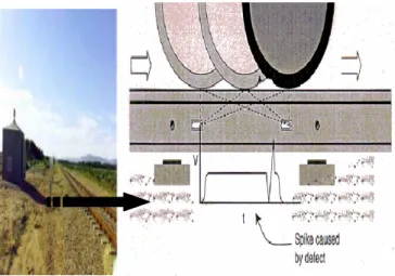
WILD systems are expensive and therefore only installed at strategic locations on the rail network. For instance, there are about twenty-four WILD sites in Canada; most of them are located on the main rail lines crossing the country. Figure 1 shows an example of the WILD system. When a train passes over a WILD site, special strain-gauges measure the impact of each wheel on the rail. An automatic tagging system reads the Id of the car as it goes over the WILD site and determines the location of the wheel being measured. A wheel’s location is specified by an axle number (1, 2, …, number of axles on the car) and the side of the wheel on the axle (right or left). The system also records additional information such as train speed, train direction, the nominal weight of the car, the name of the WILD site, and the time of the measurement. The WILD system constructs one message for each car and sends it in real-time to a central monitoring system. Table 1 shows the contents of such a message
for a car with 12 axles. The monitoring system will alert the staff if one or more wheel impact measurements exceed 140kips. The monitoring system may implement additional rules to trigger alerts but, by industry standards, a 140kips event always requires immediate action.
For this project, we use WILD data collected over a period of 17 months for a fleet of 804 large cars with 12 axles each. The dataset contains 200,808 observations like the one showed in Table 1.
Table 1. WILD data for a car with 12 axles. Attribute Description
Date/time Date and time of measurement SiteName The WILD site’s name
Dir Direction of the train (S, N, E, W) Speed Average speed of train
CarID The ID of the car NomLoad Nominal load of the car
L01 Impact for wheel on left side of axle 1 R01 Impact for wheel on right side of axle 1 L02 Impact for wheel on left side of axle 2 R02 Impact for wheel on right side of axle 2
… …
L12 Impact for wheel on left side of axle 12 R12 Impact for wheel on right side of axle 12
2.2 Maintenance Data
Most railways keep in a database detailed descriptions of all maintenance actions performed on their trains. Our partner has such a database and they provided us with a subset that contains all entries related to the fleet and period considered in this study. This subset has more than 20700 entries with a small fraction related to wheel failures. Table 2 lists the information provided in case of wheel replacements. The CarId and WheelID (axle number and axle side) identify the faulty wheel and allow us to link the failure events to corresponding WILD data. The most common types of failures as reported by the WhyMadeCode attribute are: tread shelled, flange defects, and out-of-round wheels. Tread shelled means that one or several chunks of metal (usually the size of small grape) fell out of the running surface of the wheel. The thickness and/or the height of the flange may become out of regulated limits, which will force the replacement of the wheel. Finally the out-of-round code indicates that the circumference of the wheel is not perfectly round anymore (a very small imperfection will suffice to order a wheel replacement). Wheels on a given axle are always replaced in pairs; when one fails, the other wheel on the same axle is also replaced regardless of its state. As a result, several wheels are changed without having any defect. This is noted in the database by a special WhyMadeCode attribute value. In terms of failure distribution, we observe that most wheel failures in Canada happen in winter. This is due to the fact that the accumulations of snow on the track tend to significantly accelerate the deterioration of wheels.
Table 2. Maintenance data. Attribute Description Date/time Date & time of wheel replacement JobCode Repair work completed
CarID Car Id on the train WheelID Wheel position on the car WhyMadeCode Reason for repair Description Job description Cost Cost of repair
Figure 1. Illustration of a WILD system. WILD
Before sending a train on a trip, most railways will perform a visual inspection of the wheels. Experts evaluate that these inspections catch about 75% of the wheel failures in a timely fashion. Most of the remaining 25% will be discovered during operation by WILD systems but some will go undetected with all the potential consequences mentioned in introduction.
2.3 Constructing Relevant Dataset for Data
Mining
For successful data mining, we need to gather relevant data and put it in a format that is appropriate for the target problem. In our case, the most relevant data is the one that relates to the events that we want to predict. Accordingly, we first describe how we retrieve information on past occurrences of wheel failures. Then we discuss a suitable re-organization of the WILD data and the selection of relevant subsets based on past failure occurrences.
Identification of failure events
Although it is acceptable that the new approach identifies failures already covered by the visual inspections (e.g., for validation purposes), the main benefits are in the identification of failures missed by current processes. Accordingly, we focus on prediction of high impact events. There are two ways to declare a high impact event. The first one, which we already discussed, is when a wheel impact measurement exceeds 140 kips. The second approach relies on a computed value (noted WildCal) that takes into account the nominal weight of the car, the train speed, and the impact measurement (WILDPEAK) as shown by the following equation:
Speed WILDPEAK NomLoad
WildCal= +50×
The monitoring system used by our partner computes this value as it receives the information from the WILD systems. A WildCal value greater than 170Kips will trigger the same procedure as described for the 140 kips event. Using these two definitions, we searched the collected WILD dataset and found 216 occurrences of high impact events.
We used the wheel maintenance records to validate these events by checking the time difference between wheel failure event time tw (when high impact event occurred) and its repair time tm (when
the defective wheel was replaced). We found 6 cases for which the difference between these two times was greater than 3 days. In some of 6 cases, we even observed additional WILD measurements between the high impact event and the actual repair. Being unable to really understand what happened with these cases, we decided to disregard them and focus on the 210 validated cases.
Re-representation and selection of relevant data
To maximize benefits and performance of the approach, we need to carefully select the target event to predict. In general, predicting specific events is more difficult than predicting blurred events but clear-cut predictions tend to be more valuable. For instance, in a medical application one may try to predict a specific illness or try to predict the future health of a patient. The former is likely to be more challenging but it will also produce more helpful information to the medical staff. The same reasoning
applies in our application. We may predict potential for failure for each individual wheel or we may predict potential for a wheel failure for each car, or even for the whole train. The best trade off maximizes usefulness of information for the target organization and the performance of the approach (false errors, rate of detection, etc.) After discussion with target users, we decided to select the axle level for prediction; the model will predict if a given axle is likely to suffer a wheel failure or not. Individual wheel level predictions are not required since both wheels on a given axle are replaced at the same time, as discussed above. More global predictions at the car or train level are not suitable either as the staff would have to manually find which axle(s) presents a problem.
Each observation in the initial WILD dataset (Table 1) provides information for all wheels on a given car. Since we decided to focus on the axle level, we derived a new data representation which is shown in Table 3. The first six attributes are taken from the original representation. The attribute AxleNum specifies the axle for the given observation. These seven attributes allow us to link the new representation to the initial one. The next five attributes (MaxMeas, MaxMeasPos, MinMeas, DiffMeas, AvgMeas) provide a generic way to record information on the impact from the two wheels on the same axle. Axles are installed in pairs to a platform (named a truck), which is fixed underneath the car. Due to physical propagation of impacts, it is expected that a wheel failure on a given axle will affect the behavior of the wheels on the other axle on the same truck. Such information may help predict failure so we try to capture the behavior of the wheels on the other axle of the same truck through attributes AvgMeasOAST, AvgMeasWithOASC, and DiffAvgMeasOAST.
Table 3. New WILD data representation for axle-based prediction along with time series information. Attribute Description Date/time Date and time of measurement SiteName The WILD site’s name
Dir Direction of the train (S, N, E, W) Speed Average speed of train
CarID The ID of the car NomLoad Nominal load of the car AxleNum Axle number in the car
MaxMeas Maximal WILD impact measured among the two wheels on the axle
MaxMeasPos Position that a wheel has higher impact (Right, Left)
MinMeas Minimal WILD impact measured among the two wheels on the axle
DiffMeas Difference between impacts from the two wheels on the axle
AvgMeas Average of two wheels’ impact measurements
AvgMeasOAST Average of impacts from other axle on same truck
AvgMeasWithOASC Average of all four wheels on the same truck
DiffAvgMeasOAST Difference between AvgMeasOAST and AvgMeas
SequenceID Sequence ID for each wheel failure event WithinSeqID Instance ID in a sequence
The new representation can be seen as time series data, with one series for each axle. During the analysis, we use the SequenceID attribute to distinguish the series. Once the wheels on an axle are replaced, we generate a new SequenceID value as to avoid mixing data from various axles (old and new one). Figure 2 illustrates this process for an axle with two wheel failure events at time tw1 and tw2, respectively. For this example, the
segmentation produces three sequences (s1, s2, and s3), each of
them will have a unique SequenceID value. The attribute WithinSeqID identifies each observation within a given sequence. Finally, we also compute an additional attribute named TimeToFailure to record the time between the current observation and the next wheel failure on the given axle (if any). This attribute is useful for automatic labeling and model evaluation (Section 3).
One observation in the initial WILD data format represents 12 instances in the new representation (one for each axle). Accordingly, the re-representation process converted the initial 200,808 instances into a new dataset with 2,409,696 instances. This new dataset contains 9906 distinct sequences. For building the predictive models, we consider as relevant the data collected around the high impact events. We observed that the longest time-series available in the new representation has 410 observations with an average length of 240 observations. Therefore, we decided to limit the “relevance zone” to 150 observations or instances. Since we have validated 210 failures, the resulting dataset has 31500 instances. In the following sections, we use WS to refer to this dataset.
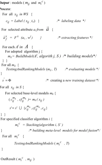
3. LEARNING METHDOLOGY
After obtaining WS, we can start building models to predict when to fix or replace a wheel. These models must accurately recognize the particular data patterns or trends that indicate upcoming wheel failures. The methodology we propose to build the predictive models from WS builds on established techniques from data mining and machine learning [10,17, 18,21]. Table 4 summarizes the notations used while Table 5 presents the pseudo code of the proposed methodology.
The methodology consists of five main processes: labeling (Label (xij , tw) ), feature extraction ( Fx ()), model building
(BuildModel() ), model evaluation (TestingAndRankingModels() ), and
model fusion (Stacking() ). The following sections describe these processes.
3.1 Labeling
We cast the wheel failure prediction problem as a binary classification task with two class values: going to fail (positive) and not going to fail (negative). Many supervised learning techniques can be used to address this task but they require that each instance in WS is pre-assigned to one of the class values. Since manual labeling of instances by domain experts is not feasible, we proceed with the automated approach introduced in [17]. The idea behind this technique is that the observable states of a physical component should be abnormal before a failure occurs. These abnormal states should be labeled as “positive” (class value 1) and the normal states as “negative” (class value 0). Precisely, we add a class attribute (cij) to each instance (xij) in
WS using the following equation:
w t if w t if ij w w c ≤ > = 1 0 (1)
where w is constant that we fix after considering two factors. The first is the amount of time suitable between a failure prediction and the actual failure. This period should be long enough to allow the staff to perform the predictive maintenance action but not too long to avoid removing components too early (which may lead to life usage reduction). In the case of wheel failure predictions, a period of one day to three-week is deemed appropriate. The second factor is the balance between the number of positive instances and the number of negative instances in the learning dataset. Without a minimal proportion of positive instances, it could be difficult for the algorithms to infer accurate models.
Table 4. The notations used in the paper.
i, j, k Counters
WS WILD dataset used for developing models
i
s The ith sequence in WS;
ij
x The j th instance in the sequencesi
ij
c Class value or label for instance xij
ij
m A base-level model built from Ai subset and the jth algorithm k m ij c , mk ij cf
Class value and its confidence identified by base-level model mk for the instance xij; (cijmk ,cfijmk )= mk (x ) ij c
i
m Meta-model for combining base-level models
ar The attribute vector in WS. ar ⊇{a1,a2...ai...}
x f
ar The vector of the feature F x
Α
Attribute space in WS,A ⊇{ar,arfx1,arxf2...} Ai The ith subset of the attribute spacetw Date/Time for instance xij
W The window size for labeling data.
Wf The window size of feature generation
Score The score for models
sci Reward score for alerts (true positive)
tw
tw1 tw2
s1 s2 s3
Figure 2. An example of data segmentation.
Wheel Failure Event 1
Wheel Failure Event 2
3.2 Feature Extraction
As in all challenging data mining applications, the quality of the representation is a key factor. While designing the WS dataset, we tried to manually craft useful features but it is possible that automated approaches could help further improve the data representation. Accordingly, we rely on constructive induction to create new powerful features that combine the initial ones [11, 19]. We also perform time-series processing to extract potentially relevant time-series characteristics. For instance, to help characterize short-term trends for each axle, we augment the representation shown in Table 3 with a new feature named MaxMeasAvg that stores the moving average of the five most recent measurements of MaxMeas from the given axle (i.e., same CarID and AxleNum as the current instance). In addition to moving averages, we also apply linear regression and Fast Fourier Transforms. We run these techniques in batch mode to generate new featuresand then add them to the representation. Finally, we apply feature selection on the augmented data representation to automatically remove correlated or irrelevant features [9, 13].
Table 5. Learning methodology.
Input: WS; (split into training dataset (S) & testing dataset (T) ) Output : models (mijand mic)
Process:
For all xijin WS {
cij = Label (xij, tw) } /* labeling data */
For selected attribute ai from
a
r
{ x f ar = Fx (ai, , wf) } /* extracting features */ For each Ai inΑ
{ For adopted algorithm j {mij = BuildModel(Ai, algorith j, S ) /* building models*/
} } For all mij {
TestingAndRankingModels (mij , T) /* evaluating models */
}
s'=Φ /* creating a new training dataset */ For all xij in S {
For selected base-level models mk{
( mk ij c , mk ij cf )= mk (x ) ij s'=s' U {cijmk,cfijmk,cij} } }
For specified classifier algorithm i { mic = Stacking(algorithm i, S’ )
} /* building meta-level models for model fusion*/ For all mic { TestingAndRankingModels (mic , T) } OutResult (mic ,mij)
3.3 Model Building
To build models, many algorithms are available including Instance-Based learning (IBk), TFIDF classifier [8], Naïve Bayes, Support Vector Machine (SVM) [12], Decision Trees, and Neural Networks. In our experiments, we tend to prefer simple algorithms such as Decision Trees and Naïve Bayes over more complex ones because they are quick and produce models that we can easily explain to our partners. We systematically apply the same algorithm several times with varying attribute subsets and cost information to obtain a set of heterogeneous but complementary base-level models. For instance, in the experimentation reported in Section 4, we selected a number of attribute subsets (noted Ai for i=1, 2,…) from the full set of
attributes (note A) and then ran the Decision Trees and Naïve Bayes classifiers using each subset. We then introduced cost-information and re-ran the above algorithms with the various attribute subsets. This process generates a number of models that will be combined in the model fusion stage (Section 3.5).
3.4 Model Evaluation
In practical applications such as ours, results must be properly evaluated. Such evaluations must fairly estimate the model's performance on new data and account for important domain-specific requirements. There are several approaches for computing the expected performance, including hold-out validation, cross-validation, and bootstrapping [7, 14]. Unfortunately, none of these approaches is adequate for our application. These approaches rely on random sampling to select instances from the population. The problem with random sampling is that it implicitly assumes that the instances are independent. Whenever this assumption generally holds, repeated analysis methods such as cross-validation and bootstrapping would probably lead to reasonably good results. However, with our application, the assumption of instance independence is simply not viable. Because of variations in system construction, operation, and maintenance, any two instances from a given system are not as independent as any two instances from two different systems. Thus, if we use data from the same wheel for training and validation, success is much more likely than if we validate using data from a different wheels.
Similarly, two instances from a particular problem (same SequenceId) will be more related than two instances from different problems. Given that the number of failures is significantly less than the total number of instances, random sampling is very likely to generate training and validation sets that contain data related to the same wheel failure event. The end result is thus an overly optimistic evaluation of the model's performance. We solve this problem by splitting the data so that training and validation instances come from different subgroups of failure events. Precisely, we ensure that all of data with a given SequenceID value will go either as part of training data or as part of the testing data but never split between the two.
We also need an adequate performance criterion for the problem at hand. In machine learning research, classifier reliability is often summarized by either error-rate or accuracy. The error rate is defined as the expected probability of misclassification: the number of classification errors over the total number of test instances. The accuracy is 1 minus the error-rate. Because some errors can be more costly than others, it's
sometimes desirable to minimize the misclassification cost rather than the error-rate. The ROC method [23], AUC (Area Under ROC Curve) [20], and cost curve [4] are very popular in practical applications since they allow the user to evaluate models based on the proportions of positive instances. Other related metrics from the information-retrieval community are precision and recall. In this context, recall is defined as the ratio of relevant documents retrieved for a given query over the number of relevant database documents; precision is the ratio of relevant documents retrieved over the total number of documents retrieved.
Unfortunately, these metrics fail to capture two important aspects of our application. The first aspect is that the usefulness of a prediction is a function of the time between the prediction and the actual replacement. Warning too early about a potential failure leads to non-optimal component use; warning too late makes proper repair planning difficult. We need an evaluation method that takes alert timeliness into account. The second aspect relates to coverage of potential failures. Because the learned model classifies each report into one of two categories (replace component; don't replace component), a model might generate several alerts before the component is actually replaced. More alerts suggest a higher confidence in the prediction. However, we clearly prefer a model that generates at least one alert for most component failures over one that generates many alerts for just a few failures. That is, the model's coverage is very important to minimizing unexpected failures. Given this, we need an overall scoring metric that considers alert distribution over the various failure cases. We shall now introduce a reward function to take into account the first aspect (timeliness of the alerts) and then we will present a new scoring metric that addresses the second aspect (coverage of failures).
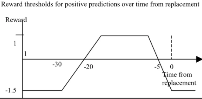
We define a reward function for predicting the correct instance outcome. The reward for predicting a positive instance is based on the number of days between instance generation and the actual failure. Figure 3 shows a graph of this function. The maximum gain is obtained when the model predicts the failure one to twenty days prior to a high wheel impact event. Outside this target period, predicting a failure can lead to a negative reward threshold, as such a prediction corresponds to misleading advice. Accordingly, false-positive predictions (predictions of a failure when there is no failure) are penalized by a reward of -1.5 in comparison to a 1.0 reward for true-positive predictions (predictions of failure when there is a failure).
The reward function in Figure 3 follows a piecewise, linear model. Such a model is convenient because it is comprehensible
to the maintenance staff and is sufficiently complex to capture the relevant information. There are several ways to improve the reward function's precision. One possibility is to use higher-order polynomials instead of straight lines. Another possibility is to try to smooth the overall function. However, according to domain experts, increased complexity is rarely needed.
Our reward function accounts for alert timeliness; to evaluate model coverage we must look at alert distribution over the different failure cases. The overall performance metric we propose to evaluate a model is as follows.
∑
= = p i i Sign sc NbrofCases NbrDtected score 1 (2) where:• p is the number of positive alerts in a given testing dataset;
• NbrDetected is the number of wheel failure events which contain at least one positive alert in the target interval (e.g. -20 and -5);
• NbrofCase is total number of wheel failure events in a given testing dataset;
• Sign is the sign of
∑
= p i i sc 1
. When Sign <0 and NbrDetected=0, score is set to zero; and
• sci is calculated with the reward function above.
3.5 Model Fusion
One way to enhance performance is to combine multiple heterogeneous base-level models/classifiers into a multiple classifier system (MCS) [15]. Many research results have shown that an MCS improves the performance over a single base-level model [2, 3, 5, 6, 22, 26]. Several methods exist for combining multiple models, including Bagging, Boosting, Randomization [3], Voting [26], Stacking, Rule-based [5], and others [5]. In our experiments, we focused on Stacking [2] as it allows efficient and simple combinations of heterogeneous models.
In stacking, we rely on meta-models to combine multiple base-level models. The first step is to select several base-base-level models ( m1,m2,...mk ) from the developed heterogeneous models by
ranking them with our evaluation approach. In the second step, we generate a dataset that contains the predictions of all selected models m1,m2,...mkfor each instance {Xij,cij} in the training set. We note these predictions mk
ij m ij m ij c c
c1, 2... . We also add to the new
dataset the confidence factors for these predictions (noted
k m ij m ij m ij cf cf
cf 1, 2... ) plus the initial label (cij). Accordingly, the new
dataset (noted
s
'
) has the following attributes { mk ij m ij m ij c c c 1, 2... , k m ij m ij m ij cf cfcf 1, 2... , cij}. We then use
s
'
as a training dataset to learn meta-models. We use Decision Trees and Naïve Bayes to learn the meta-models but other algorithms could also be suitable. Finally, we rank the meta-models by evaluating their performance on the testing data. We select the meta-model with the highest score to form a MCS capable of combining several base-level models to predict train wheel failures.Reward thresholds for positive predictions over time from replacement
Figure 3. The reward function for positive predictions.
0 1 -1.5 Reward -5 -20 1 -30 Time from replacement
4. EXPERIMENTS
In this section, we discuss a large-scale experiment using the proposed methodology. We first describe the parameter settings and then discuss the actual experiment along with the results. For this experiment, we used SAS to implement data generation, model evaluation, and result analysis. The WEKA system was used to construct the models.
4.1 Parameter settings
The methodology proposed has a number of key parameters. In this section, we describe the settings of these parameters as well as the process leading to the chosen values.
• The size of the target window for data labeling
We carried out simplified experiments by varying only the size of the target window for labeling (w). We investigated window sizes from 15 to 30 and found that
w=20 (i.e., predictions up to 20 days prior to failures)
offers the best compromise. This value leads to an adequate balance between positive and negative examples and is perfectly acceptable for railways.
• The window size for feature extraction
For simplicity, we added only two types of new features: moving average features (Fmv ) and generalized linear regression features (Fgl). The computation of both Fmv
and Fgl requires a window size value (wf ) that specifies
the length of the sub-sequence to consider when computing a new feature value. For instance, wf = 8 means that any new feature value depends on the past 7 observations plus the current one. We conducted feature extraction experiments using different window sizes (wf
= 8, 12, 16, 20, 24…) and concluded that the most suitable window sizes for Fmv and Fgl are 8 and 16, respectively. We only extracted features for a few of the key attributes such as MaxMeas and AvgMeas.
• The attribute subsets and attribute selection
To optimize performance, we evaluated various subsets of attributes using the training data. We kept the four most promising subsets (noted A1,A2,A3,A4 ) with different number of attributes. We applied the selected learning algorithms on these four subsets to construct a set of heterogeneous base-level models.
• The cost information
To obtain an adequate balance between false positive and false negative errors, we decided to also build models with non-default cost information. The decision trees (J48) and naïve Bayes implementations provided in the WEKA system can take cost information into account when building the models. The user provides the cost information through a cost-matrix that specifies the penalty for false positives and false negatives.
Unfortunately, we had to identify the cost-matrix ourselves since the domain experts could not easily provide us with such information. After several experiments, we decided to use the following cost-matrix since it leads to a fairly low false positive rate without significant negative effect on the detection of failures:
= 1 2 0 1 1 0 cos tMatrix
This matrix gives penalty 2 for false positives and 1 for false negative.
4.2 Model-building Experiment
We divided WS into training and a testing datasets noted S and
T, respectively. S contains 22083 instances associated to 145
wheel failure events or sequences. Thas 9337 instances for 65 sequences. After setting the parameters as explained above, we learned the heterogeneous base-level models and then built meta-models to combine the low-level meta-models.
4.2.1 Building heterogeneous base-level models
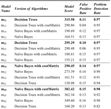
As shown in Figure 4, 16 heterogeneous base-level models (mij with i=1,2,3,4 and j=1,2,3,4) were built by applying different algorithms to different datasets formed from A1,A2,A3,A4.
We computed the performance of each model using Equation 2 and then ranked the models for each subset of attributes. Table 6 shows the results. Since the testing dataset contains 9337 instances and 65 sequences, the potential score values are from -9500 to 1200. The higher the score is, the better the performance of a model is. We also report false positive rate and problem detection rate. The problem detection rate is the number of failures detected over the 65 wheel failures events contain in the testing dataset T. The false positive rate is calculated based on the confusion matrix from each model. Highlighted lines in Table 6 identify the best models within each group.
Attribute Space (
Α
) A1 A2 A4 A3 Decision Trees Naïve Bayes Decision Trees with costMatrix Naïve Bayes with costMatrix mi1 mi2 mi3 mi4 i = 1, 2, 3, 44.2.2 Building meta-models
To build the meta-models, we selected the best 4 base-level models from Table 6 (i.e., m11, m21, m34 and m44). We applied these models to all instances {Xij} in S to generate
44 34 21 11, , , m ij m ij m ij m ij c c c c and 11, 21, 34, m44 ij m ij m ij m ij cf cf cf
cf , and to create a new
training dataset s'⊇{ 11, 21, 34, m44 ij m ij m ij m ij c c c c , 11, 21, 34, m44 ij m ij m ij m ij cf cf cf cf ,cij }.
Then we applied the two versions (with and without cost) of decision trees and naive Bayes on S’ to build meta-models. Like what we did to evaluate the base-level models, we computed the score of each meta-model and then ranked them. Table 7 shows the result. Finally, we selected the meta-model mc
1(since it has
the highest score) to form a MCS that combines four base-level models for wheel failure predictions. Figure 5 shows the architecture of the MCS obtained.
Table 6. Ranking of base-level models.
Model
Name Version of Algorithms
Model Score False Positive Rate Problem Detection Rate m11 Decision Trees 315.58 0.11 0.97
m13 Decision Trees with costMatrix 290.86 0.04 0.95
m14 Naïve Bayes with costMatrix 198.69 0.12 0.97
m12 Naïve Bayes 164.51 0.13 0.97
m21 Decision Trees 295.29 0.10 0.97
m23 Decision Trees with costMatrix 290.48 0.06 0.95
m24 Naïve Bayes with costMatrix 188.81 0.15 0.97
m22 Naïve Bayes 155.21 0.15 0.97
m34 Naïve Bayes with costMatrix 290.45 0.14 0.97
m32 Naïve Bayes 273.39 0.16 0.98
m33 Decision Trees with costMatrix 161.51 0.12 0.91
m31 Decision Trees 138.08 0.15 0.94
m44 Naïve Bayes with costMatrix 382.42 0.15 0.98
m43 Decision Trees with costMatrix 362.34 0.13 0.92
m42 Naïve Bayes 349.60 0.16 0.98
m41 Decision Trees 160.20 0.13 0.82
Table 7. Ranking of meta-models.
Meta-Model Name
Version of Algorithms Model
Score False Positive Rate Problem Detection Rate c m1 Decision Trees 698.49 0.08 0.97 c
m2 Decision Trees with costMatrix 650.94 0.08 0.97
c
m3 Naïve Bayes with costMatrix 643.35 0.12 0.98
c
m4 Naïve Bayes 622.67 0.13 0.98
We are now developing a real-time wheel-monitoring prototype based on the constructed MCS. We plan to evaluate this prototype through a field trial. The monitoring system receives the WILD data in real-time and transforms it into our representation. Feature extraction is also applied to the selected attributes. Each base-level model is provided with the attributes it
requires (a subset amongA1,A2,A3,A4) and returns prediction on
failure along with confidence. All base-level model outputs ( 11, m11 ij m ij cf c , 21, m21 ij m ij cf c , 34, m34 ij m ij cf c , 44, m44 ij m ij cf
c ) are given as input to the
meta-model c
m1. The monitoring system will use the output of the meta-model (our MCS) to decide when to alert staff of upcoming wheel failures.
5. DISCUSION AND OPEN ISSUES
To the best of our knowledge, this paper describes the first application of KDD for prognostics of train wheel failures. The lack of comparable work prevents us from contrasting our results with ones from other researchers. Instead, we evaluate the significance of our work by assessing the benefits over the most advanced use of WILD data in the railway industry.
Many railways have recently started to use the WILD data and threshold-based approach [25] for predictive maintenance of wheels. This approach uses a set of pre-determined thresholds to alert staff of potential for future 140kips events. Commonly used thresholds are 65kips, 80kips, and 90kips. In practice, most railways will start looking for a suitable time to replace a wheel once it has exceeded the 90kips level a couple of times. Depending on schedule, shop’s work load, and the availability of new wheels, it may take several days or even weeks before the wheel gets replaced. A high number of 90kips alerts will increase priority on the repair while 80kips and 65kips alerts will often be ignored.
Since the railway was not applying the above procedure during the period of time considered in this project, we have been able to use the available data to study the ability of the 90kips threshold-based approach to prevent 140kips events during operation. We found two major problems with this approach. First, we observed that a large number of 90kips events never lead to 140kips events or wheel replacements (even after several months). For all of these cases, the 90kips threshold-based approach would have generated false alerts and potentially cause the replacement of many good wheels. Second, focusing on the cases for which we actually observed a 140kips event, we found that the time it takes from a 90kips event to a 140kips event varies so much that it becomes impossible to determine how long the organization has to perform the repair. For examples, we found a number of cases for which a 140kips event immediately follows the corresponding
M11 M21 M34 M44
c
m
1
A1 A2 A3 A4 11 11, m ij m ij cf c 21 21, m ij m ij cf c 34 34, m ij m ij cf c 44 44, m ij m ij cf c c c m ij m ijcf
c ,
Figure 5. An MCS constructed using a meta-model and 4 base-level models.
ij
90kips event while in other cases the delay between the two events was greater than a year. This means that for some cases, the 90kips alerts are raised too late to allow any predictive maintenance actions while in other cases they were way too early. Our approach resolves this issue through sophisticated data mining models that closely match the various failure patterns and raise alerts in a timely manner. Indeed, as shown in Table 7, the proposed methodology detected more than 97% of all wheel failures in the test data by raising warnings during the selected time-frame (i.e., from 1 day to 20 days in advance). The false alert rate was curbed at a relatively low level (less than 8%). Comparing results in Table 6 with the ones in Table 7, we observed that the meta-model boosted the performance of base-level models through a much higher score and a lower false alert rate.
The experimental results demonstrated that the developed methodology is capable of building high-quality models for predicting train wheel failures but there are still a number of open problems:
• Alternative approach to trade-off failure detection and false alert rates
An ideal model or classifier should detect all failures without generating any false alert. In real-world applications, such a model is rarely feasible. In general, when we try to increase the detection rate, we obtain a higher false alert rate. For instance, both m42 and the m44 in Table 6 have the highest detection accuracy (98%), but they also generate more false alerts than the other models (15% of false positives). In our approach we used cost information as a way to balance the failure detection rate and the false alerts but alternative techniques are suitable. In particular, it would be useful to have a technique that could automatically optimize the trade-off without requiring a cost-matrix.
• Improvement of data quality
Data quality includes the quality of operational data and the quality of maintenance data. The operational data comes from the WILD systems. To build the models, we assumed that all WILD data was reliable but further analysis suggested that some of the WILD sites were not properly calibrated. To enhance performance, additional efforts should be deployed to ensure adequate precision in data acquisition. Our methodology could also be expended with automatic data validation techniques to monitor data quality before learning the models.
The quality of the maintenance data directly affects the identification of the wheel failure events, which in turn determine the data to be used for building the models. In this particular application, it was sometimes difficult to identify the exact location of the wheel that has been replaced. The cars on train have 12 axles for a total of 24 wheels. To identify a particular wheel location, the maintenance staff enters the number of the axle (1 to 12) and the side of the faulty wheel (right or left) in free form text. Unfortunately, we found many inconsistencies and errors in this text. For instance, technicians used many symbols to refer to the axle number 10 such as: `a', `10', `x', `0x'. The same problem also exists for other axles above 10. Moreover, we found that the staff sometime entered the wrong axle number (e.g., 6 or 8
instead of 7) or wrong side (left instead of right). These errors can negatively influence the modeling process by making it construct failure models that fit non-failing wheel data. We try to deal with errors in wheel location through extensive manual validation. When the ambiguity is too high, we generally ignored the case and ensured that potentially related sensor data was not included in the model-building experiments. To ensure good predictions, it is desirable that the technicians are aware of the potential consequences of errors in maintenance data and are provided with proper validation tools to ensure consistency.
• Cost-based analysis of the developed models
Our model evaluation approach takes the timeline of the alerts and problem coverage into consideration but it does not compute the potential business value of a given model to predict wheel failures. Ideally, we would like an extension of the current method that takes into accounts the various costs (undetected failures, early replacement, false alerts, and implementation of the models) and returns the expected gain in dollars. However, this may not be practical as organizations may be unable to adequately evaluate these costs. We should therefore also investigate other alternatives.
6. CONCLUSIONS
In this paper, we introduced a comprehensive KDD methodology to build models to predict high impact wheel events before they disrupt operation. The proposed methodology innovates in key data-mining areas such as data representation, automatic labeling, model fusion, and model evaluation. Most of the steps are generic and can be reused in other circumstances such as in medical and environmental applications. We evaluated the feasibility of the methodology through a large-scale experiment in which we build a set of the heterogeneous base-level models and a set of meta-models to implement model fusion. After combining four base-level models, we have successfully constructed a Multiple Classifier System (MCS) capable of predicting 97% of wheel failures while maintaining a reasonable false alert rate (8%). Such results clearly show the great potential of this innovative application of data mining in the railway industry. Our future work includes a field trial to further evaluate the usefulness of the technology developed and additional research on the open issues discussed.
7. ACKNOWLEDGMENTS
Many people at National Research Council have contributed to this project. Special thanks go to Bob Orchard, Chris Drummond, Marvin Zaluski, Elizabeth Scarlett, George Forester, Jon Preston-Thomas, and Mike Krzyzanowski for their support, valuable discussions and suggestions.
8. REFERENCES
[1] Aha, D., Kibler D. and Albert, M., Instance-based learning algorithm. Machine Learning, Vol.6, 2004, 37-66 [2] Conversano, C., Siciliano, R. and Mola, F. , Supervised
Classifier Combination through Generalized Additive Multi-model, The Proceeding of International Workshop in Multiple Classifier Systems (MCS2000), 2000, 167-176
[3] Dietterich, T., An experimental Comparison of three methods for Constructing Ensembles of Decision Trees: Bagging, Boosting and Randomization, Machine Learning, Vol. 40, 2000, 139-158
[4] Drummond, C. and Holte, R., Explicitly Representing expected cost: an alternative to ROC representation, Proceedings of the 6th ACM SIGKDD International
Conference on Knowledge Discovery and Data Mining, New York, 2000, 198-207
[5] Duin, R. and Tax, D., Experiments with Classifier Combining Rules, The Proceeding of International Workshop in Multiple Classifier Systems (MCS2000), 2000, 16-29
[6] Dzeroski, S. and Zenko, B., Is Combining Classifiers with Stacking Better than Selecting the Best One?, Machine Learning, Vol.54, 2004, 255-273
[7] Efron, B., Estimating the Error Rate of a Prediction Rules: Improvement on Cross Validation, J of American Statistical Association, Vol. 78, 1983, 316-331
[8] Grossman, D. and Frieder, O., Information Retrieval: Algorithm and Heuristics, Kluwer Academic, 1998 [9] Hall, M., Correlation-based Feature Selection for Discrete
and Numeric Class Machine Learning, Proceedings of the 17th International Conference on Machine Learning, 2000, 359-366
[10] Han, J. and Kamber, M., Data Mining: Concepts and Techniques, Morgan Kaufmann Publishers, 2001 [11] Harries, M., Sammut,C. and Horn, K., Extracting Hidden
Content, Machine Learning, Vol. 32, 1998, 101-126 [12] Joachima, T., Text Categorization with Support Vector
Machine: Learning with Many Relevant Features, Proceedings of the 10th European Conference on Machine Learning, 1998, 487-494
[13] Kira, K. and Rendell, L., A Practical Approach to Feature Selection, Proceedings of the 9th International Conference on Machine Learning, 1992, 249-256
[14] Kubat, M., Holte, R.C. and Matwin, S., Machine Learning for the Detection of Oil Spills in Satellite Radar Images, Machine Learning, Vol. 30, 1998, 195-215
[15] Lam, L., Classifier Combinations: Implementations and Theoretical Issues, The Proceeding of International Workshop in Multiple Classifier Systems (MCS2000), 77-86
[16] Lechowicz, S. and Hunt, C., Monitoring and Managing Wheel Condition and Loading,
http://www.ntsb.gov/events/symp_rec/proceedings/authors/le chowicz.pdf
[17] Létourneau, S., Famili, F., Matwin, S. Data mining for prediction of aircraft component replacement. IEEE Intelligent Systems Journal, Special Issue on Data Mining. December 1999. 59-66
[18] Létourneau, S. Data Mining for Maintenance of Complex Systems, SIGART/AAAI Doctoral Consortium, Proceedings of the National Conference on Artificial Intelligence (AAAI). Madison, Wisconsin, USA. July 27, 1998.
[19] Létourneau, S., Identification of Attribute Interaction and Generation of Globally Relevant Continuous Feature in Machine Learning, Ph.D thesis, School of Information Technology and Engineering, University of Ottawa, 2003 [20] Ling, C.X., Huang, J., Zhang, H. AUC: a Statistically
Consistent and more Discriminating Measure than Accuracy, Proceedings of IJCAI 2003, 519-524
[21] Mitchell, T.M., Machine Learning, WCG McGraw-Hill, 1997
[22] Opitz, D. and Maclin, R., Popular Ensemble Methods: An Empirical Study, Journal of Artificial Intelligence Research Vol. 11, 1999, 169-198
[23] Provost F.,Fawcett, T. Analysis and Visualization of Classifier Performance: Combination under Imprecise Class and Cost Distributions, Proceedings of International Conference on Knowledge Discovery and Data Mining (KDD97), 1997
[24] Salient Systems Inc., Preventing Train Derailment, http://www.salientsystems.com
[25] Technical report, Advanced Technology Safety Initiative: Equipment Health Management System, Association of American Railroads, August 24, 2004
[26] Tsoumakas, G., Katakis, I., and Blahavas I., Effective Voting of Heterogeneous Classifiers, Proceedings of the 15th European Conference on Machine Learning (MCML2004), Pisa, Italy, 465-476
[27] Witten, I. And Frank, E., Data mining: Practical machine learning tools and techniques with Java implementations, Morgan Kaufmann, San Francisco, CA, 2000