Capitalising on covariates in cluster-randomised experiments

(1)

cluster-randomised experiments

Jan Vanhove*

31August 2020

Abstract

In cluster-randomised experiments, participants are randomly as-signed to the conditions not on an individual basis but in entire groups. For instance, all pupils in a class are assigned to the same condition. This article reports on a series of simulations that were run to determine (1) how the clusters (e.g., classes) in such experiments should be assigned to the conditions if a relevant covariate is available at the outset of the study (e.g., a pretest) and (2) how the data the study produces should be analysed if researchers want to maximise their statistical power while retaining nominal Type-I error rates. The R code used for the simulation is freely accessible online, allowing researchers who need to plan and analyse a cluster-randomised experiment to tailor the simulation to the specifics of their study and determine which approach is likely to work best.

1 Introduction

In fields such as education and medicine, it is often impractical to randomly assign individual participants to the experiment’s conditions. Instead, the participants are assigned to conditions in intact groups. For instance, entire school classes may be randomly assigned to the experimental conditions in such a way that pupils from the same class are always assigned to the same condition. Such experiments are called cluster-randomised experiments. The goal of this article is to provide actionable advice to researchers who need to design a cluster-randomised experiment and analyse its data.

When random assignment took place at the cluster level rather than at the *_{jan.vanhove@unifr.ch. https://janhove.github.io. University of Fribourg, Department of} Multilingualism, Rue de Rome 1, 1700 Fribourg, Switzerland.

(2)

individual level, the analysis needs to take this into account. Members belonging to the same cluster (e.g., pupils in the same class) tend to be somewhat more alike than individuals belonging to different clusters. This induces a correlation in the performance of participants in the same cluster, the strength of which is expressed by the intraclass correlation (ICC). The ICC is computed as the ratio of the variance between clusters to the overall variance: ICC = σ 2 between σ_total2 = σ_between2 σ_between2 + σ_within2

Ignoring such clustering dramatically invalidates the results of the analysis, as illustrated in Figure 1 on the following page. When the clustering is appropriately taken into account, cluster-randomised experiments have less statistical power and less precision than experiments in which the same total number of participants was randomly assigned on an individual basis (other things equal). Just as with individually-randomised experiments, however, the power and precision of cluster-randomised experiments can be increased by obtaining more data (more observations per cluster, but especially more clusters) or by reducing the residual variance. The latter can be accomplished by leveraging pre-treatment covariates (e.g., pretests; Bloom, Richburg-Hayes & Black 2007; Hedges & Hedberg 2007; Klar & Darlington 2004; Moerbeek 2006; Murray & Blitstein 2003; Raudenbusch, Martinez & Spybrook 2007; Schochet 2008). But while I have read about numerous strategies for including covariates in the analysis of cluster-randomised experiments, I have found little discussion about the relative merits and drawbacks of these different strategies. In this article, I want to provide such discussion.

I take the perspective of a researcher who, for practical reasons, needs to carry out a cluster-randomised experiment and has to make do with a fixed number of clusters (e.g., 12 classes) of a given size and who has some relevant information about the participants to their disposal at the outset of the study (e.g., a pretest score). This researcher needs answers to two important questions:

1. How should I assign the clusters to the experiment’s conditions? 2. How should I analyse the data?

Throughout, I will assume that this researcher wants to maximise the experi-ment’s statistical power.

(3)

0.00 0.05 0.10 0.15 0.20 0.25 0.0 0.2 0.4 0.6 0.8 ICC Ty p e -I e rr o r ra te

Nominal Type-I error rate (0.05)

m = 100 m = 50

m = 20

m = 10

m = 5

Figure 1:Type-I error rates for cluster-randomised experiments when anal-ysed by means of a t-test on the participants’ scores (i.e., without taking the clustering into account) as a function of the intraclass correlation coeffi-cient (ICC) and the number of participants per cluster (m). For this graph, the number of clusters was fixed at 10, but the Type-I error rate differs only slightly for different numbers of clusters. This figure is redrawn from Vanhove (2015) and is based on a formula provided by Hedges (2007).

Below, I will first discuss three options for assigning clusters to the conditions as well as several options for analysing the data when a pre-treatment covari-ate is available. I will then report on a series of simulations in which I pitted different assignment and analysis methods against each other. The large number of combinations of assignment options, analysis methods, and simu-lation settings unfortunately make for tedious reading, so let me anticipate the key findings:

1. In terms of statistical power, the differences between the three methods for assigning clusters to conditions that are discussed in this article are minute.

2. A fairly simple but powerful way to analyse the data is to compute the mean outcome and mean covariate score for each cluster and then compare the intervention and control clusters’ mean outcomes in an ancovawith the cluster mean covariate scores as the covariate.

2 Methods for assigning clusters to conditions

The assignment of clusters to conditions can be done without taking the covariate into account. If the assignment is effected at random but under the restriction that there should be an equal number of clusters per condition, this amounts to a completely randomised design at the cluster level.1

The covariate 1

Alternatively, the clusters can be assigned using simple randomisation. This means that every cluster is assigned with the same probability (typically 50%) to either condition. In this

(4)

can still be used during the analysis even if it was ignored when assigning the clusters to the conditions.

The second option is to adopt a blocked randomised design at the cluster level (see Raudenbusch, Martinez & Spybrook 2007). For each cluster, the average covariate score is computed, and the clusters are ranked in descending order on the average covariate score. Then, pairs (‘blocks’) are formed by grouping ranks 1 and 2, ranks 3 and 4, etc. Within each pair, one cluster is randomly assigned to the control condition and one to the intervention condition. For an experiment with six clusters, one possible assignment is as follows:

• Rank 1: intervention • Rank 2: control • Rank 3: intervention • Rank 4: control • Rank 5: control • Rank 6: intervention Another is this: • Rank 1: intervention • Rank 2: control • Rank 3: control • Rank 4: intervention • Rank 5: intervention • Rank 6: control

However, the following assignment would not be possible since, in two pairs (ranks 3 and 4, and ranks 5 and 6), both clusters are assigned to the same condition. • Rank 1: intervention • Rank 2: control • Rank 3: control • Rank 4: control • Rank 5: intervention • Rank 6: intervention

In a completely randomised design, large imbalances in the covariate can occur between the experimental conditions due to chance. In a blocked case, one could end up with four clusters in the intervention condition and eight in the control condition. Typically, simple randomisation incurs some loss of statistical power compared to complete randomisation, so I will leave simple randomisation out of consideration.

(5)

randomised design, such large imbalances are prevented from occurring (see Hayes & Moulton 2009). The advantage of having a fairly balanced covariate distribution between the conditions is that it makes covariate adjustment more effective.

A third option is to adopt the alternate ranks design (Dalton & Overall 1977). The clusters are again ranked according to their average covariate scores. They are then assigned to the control or intervention condition in an ABBAABB... fashion. Whether it is A or B that stands for ‘intervention’ or ‘control’ is randomly determined. In an alternate ranks design, there are only two possible assignments; in the case of an experiment with six clusters, these are: • Rank 1: intervention • Rank 2: control • Rank 3: control • Rank 4: intervention • Rank 5: intervention • Rank 6: control and • Rank 1: control • Rank 2: intervention • Rank 3: intervention • Rank 4: control • Rank 5: control • Rank 6: intervention

I have not seen any discussion of the alternate ranks design in the context of cluster-randomised experiments, but their use has been advocated in experiments where participants are assigned on an individual basis (Dalton & Overall 1977; Maxwell, Delaney & Hill 1984; McAweeney & Klockars 1998). The alternate ranks design more strongly guarantees that the distribution of the covariate is balanced between the experimental conditions than the blocked randomised design, possibly rendering covariate adjustment even more effective. Particularly for experiments with a small number of clusters, where chance can otherwise more easily give rise to covariate imbalance, the alternate ranks design may be advantageous, which is why I included it in the simulations.

(6)

control intervention 2 7 9 1 4 10 11 6 5 8 3 12 -2 -1 0 1 2 Class Pos tt es t sc ore -2 -1 0 1 2 -2 0 2 Pretest score Pos tt es t sc ore

condition control intervention

Figure 2:The simulated data set used to illustrate the different analytical approaches. Left: The posttest scores in the different classes. Right: The relationship between the pretest and posttest scores in the entire data set.

3 Methods for taking the covariate into account in the

analysis

Here I briefly discuss 25 possible ways in which data from a cluster-randomised experiment can be analysed when a pre-treatment covariate (e.g., a pretest) is available. I will not discuss different methods for analysing cluster-randomised experiments that ignore the pre-treatment covariate (see Johnson et al. 2015 for a comparison of some such methods). To illustrate the approaches in which a covariate is considered, I generated a data set with 12 classes with 10 to 29 pupils per class (223 pupils in total). That is, the cluster sizes were not balanced, but they did not vary over orders of magnitude either. This, I think, is fairly typical of real-life cluster-randomised experiments, at least in my own field (applied linguistics). A covariate in the form of a pretest score was available, and the classes were assigned to the conditions by block randomisation as discussed above (six classes per condition). Figure 2 shows the data set. I also provide R code to make sure that the procedures are outlined unambiguously.

If you want to follow along with with the examples below, you can download this simulated data set from https://osf.io/wzjra/. It contains the variables block(specifying the block within which the classes were randomly allocated to the conditions), class, pretest (the individual participants’ pretest scores), and outcome (the individual participants’ outcome). You will also need R with the tidyverse, lme4 and lmerTest packages installed and loaded. Note that I do not recommend actually trying out several different analyses on the same data and then picking one that seems to work best. In fact, the aim of this article is to help researchers make an informed decision about how to analyse their study before the data are in.

(7)

intervention control -0.2 0.0 0.2 1 (n = 12) 9 (n = 19) 2 (n = 10) 4 (n = 25) 7 (n = 24) 10 (n = 28) 11 (n = 11) 12 (n = 20)5 (n = 17) 8 (n = 29) 6 (n = 15) 3 (n = 13)

Mean residualised posttest score per class

C

las

s

Figure 3: The outcome scores were first regressed against the covariate scores in a simple linear regression model that did not take either clustering or the experimental condition into account. The estimated residuals from this model were then averaged per class.

3.1 Analyses on cluster-level summaries

The first class of analyses are run not on the individual data points but on cluster-level summaries of them.

3.1.1 Cluster mean residualised outcomes

Hayes & Moulton (2009) (p. 182) propose the following method for analysing cluster-randomised experiments when a pre-treatment covariate is available. First, regress the outcomes against the covariate in a simple linear model that ignores the clusters. Then, obtain the residuals from this model and calculate the mean residual per cluster. Finally, analyse these cluster mean residuals with a t-test.

The code below shows how this analysis can be run on the simulated data set. (I use the lm() function rather than t.test() as it directly outputs the estimated treatment effect and its standard error.) The cluster mean residuals are shown in Figure 3. This analysis yields an estimated treatment effect of

ˆβ = 0.24±0.09 (t(10) = 2.6, p = 0.03).

# Regress outcome against pretest and obtain residuals

d$residual <- lm(outcome ~ pretest, d) %>% resid()

# Compute mean outcome and mean residual per class

d_per_class <- d %>%

group_by(class, condition) %>% summarise(

(8)

.groups = "drop"

)

# Fit model

m <- lm(mean_residual ~ condition, data = d_per_class)

summary(m)$coefficients

## Estimate Std. Error t value Pr(>|t|)

## (Intercept) -0.13 0.066 -2.0 0.077

## conditionintervention 0.24 0.094 2.6 0.028

# Run ’summary(m)’ for the full summary, # including degrees of freedom

3.1.2 Cluster mean outcomes with cluster mean covariate scores

A second option is to average both the outcome and the covariate scores per cluster and then analyse the cluster mean outcomes in an ancova with the cluster mean covariate scores as the covariate. While I did not find any recommendations for this method in the literature, it is the ancova counterpart to the strategy of submitting the cluster means to a t-test (e.g., Barcikowski 1981), and it seems useful to investigate the statistical properties of this kind of analysis.

The code below shows how such an analysis can be run in R; also see Figure 4. The estimated intervention effect according to this analysis is ˆβ = 0.24±0.10 (t(9) = 2.5, p = 0.03).

# Summarise by cluster

group_by(class, condition) %>% summarise(

mean_outcome = mean(outcome),

mean_pretest = mean(pretest),

n = n(),

.groups = "drop"

)

# Fit model

m <- lm(mean_outcome ~ mean_pretest + condition,

data = d_per_class)

(9)

-0.25 0.00 0.25 0.50

-1.0 -0.5 0.0 0.5

Mean pretest score per class M ean pos tt es t sc ore per c las s

condition control intervention

Figure 4: Both the outcome and covariate scores were first averaged per class. The dotted and solid lines show the fit of a regression model (or ancova) with condition (intervention vs. control) and the cluster mean covariate scores as predictors and the cluster mean outcomes as the outcome variable.

## (Intercept) 0.15 0.070 2.1 0.0620

## mean_pretest 0.48 0.119 4.0 0.0031

3.1.3 Cluster mean outcomes with assignment blocks

The standard method for analysing a blocked randomised design is to include the blocking factor in the model, either as a fixed effect in an ordinary linear model (Faraway 2005, Chapter 16) or as a random effect in a mixed-effects model (Faraway 2006, Section 8.4). We can apply the same analysis to cluster means of blocked cluster-randomised experiments. When the design is balanced (i.e., when no clusters were lost) and the mixed-effects model does not obtain a singular fit, accounting for the blocks by means of a random effect yields the same result for the intervention effect as accounting for the blocks using fixed effects. In fact, you would also obtain the same result by running a repeated-measures anova on the cluster means (with condition as a within-block factor) or by applying a paired t-test on the cluster means (cluster means paired per block). In the following, I will only account for the blocks using fixed effects when the cluster means are analysed. For the simulated dataset, this approach yields an estimated intervention effect of

ˆβ = 0.27±0.06, t(5) = 4.7, p = 0.005; also see Figure 5.

# Calculate mean outcome per class

group_by(block, class, condition) %>% summarise(

(10)

6 5 4 3 2 1 -0.25 0.00 0.25 0.50 cluster mean outcome

bloc

k

condition control intervention 6 5 4 3 2 1 0.0 0.1 0.2 0.3 0.4 diﬀerence between intervention and control class within each block

bloc

k

Figure 5: Within each block of the simulated blocked cluster-randomised experiment, the intervention class outperformed the control class on the outcome.

.groups = "drop"

)

# Block as fixed effect

m <- lm(mean_outcome ~ block + condition, data = d_per_class)

## (Intercept) 0.194 0.076 2.55 0.0514 ## block2 0.150 0.100 1.51 0.1912 ## block3 0.117 0.100 1.18 0.2911 ## block4 -0.072 0.100 -0.72 0.5024 ## block5 -0.172 0.100 -1.72 0.1452 ## block6 -0.553 0.100 -5.56 0.0026 ## conditionintervention 0.270 0.057 4.70 0.0054

This analysis cannot be run if the experiment used complete randomisation or an alternate ranks design rather than block randomisation.

3.2 Analyses on individual-level data

One possible problem with analyses on cluster-level summaries may occur when the clusters differ in size. Measurement error affects the means of small clusters more than of large clusters. When cluster sizes vary, the variance about the different cluster means will consequently be different, which violates the homoskedasticity assumption of the general linear model (including Student’s t-test and ancova). One solution to this problem is to

(11)

analyse the individual-level data in a multilevel (or mixed-effects) model that explicitly accounts for the clusters (also see Klar & Darlington 2004, models 3 and 4). In the following, I will discuss a couple of variations of this kind of model. In the next section, I will discuss another solution, which involves analysing cluster-level summaries while weighting the clusters by a function of their size.

3.2.1 Multilevel model with individual covariate scores

The individual-level data from a cluster-randomised experiment can be fitted in a multilevel (or mixed-effects) model with the individual covariate scores as a covariate and with by-cluster random intercepts to take the clustering into account. Hayes & Moulton (2009) recommend the use of multilevel models only when there are more than 15–20 clusters per condition (!), though it is not clear if their advice also applies to multilevel models that include a covariate.

For the simulated dataset, a multilevel model with condition and the indi-vidual covariate scores as fixed effects and random intercepts for class (fitted using the lme4 and lmerTest packages for R) estimated the intervention effect as ˆβ = 0.21±0.10 (t(220) = 2.2, p = 0.03, using Satterthwaite degrees of freedom):

library(lmerTest)

m <- lmer(outcome ~ pretest + condition + (1|class), data = d)

## Estimate Std. Error df t value Pr(>|t|)

## (Intercept) 0.18 0.066 220 2.8 5.5e-03

## pretest 0.54 0.038 220 14.3 3.6e-33

## conditionintervention 0.21 0.096 220 2.2 2.7e-02

3.2.2 Multilevel model with both individual and cluster mean covariate

scores

Individual covariate scores and cluster mean covariate scores can be fitted jointly in a multilevel model (see Klar & Darlington 2004, model 4). In our example, this yields an estimated intervention effect of ˆβ = 0.21±0.10 (t(219) = 2.2, p = 0.03).

d_per_class <- d %>% group_by(class) %>% summarise(

(12)

.groups = "drop"

)

# Add this information to the large dataset

d <- d %>%

left_join(d_per_class, by = "class")

m <- lmer(outcome ~ pretest + mean_pretest + condition +

(1|class), data = d)

## Estimate Std. Error df t value Pr(>|t|) ## (Intercept) 0.182 0.066 219 2.8 6.3e-03

## pretest 0.546 0.039 219 13.8 9.5e-32

## mean_pretest -0.084 0.140 219 -0.6 5.5e-01 ## conditionintervention 0.212 0.096 219 2.2 2.8e-02

3.2.3 Multilevel model with assignment blocks

While I have not found any examples of this, the blocking factor in a blocked cluster-randomised design could conceivably be taken into account in a multilevel model. For the simulated dataset, taking the blocks into account using fixed effects yields an estimated intervention effect of ˆβ = 0.25±0.13 (t(216) = 1.9, p = 0.06).

m <- lmer(outcome ~ block + condition + (1|class), data = d)

## (Intercept) 0.208 0.19 216 1.08 0.280 ## block2 0.166 0.23 216 0.73 0.468 ## block3 0.089 0.24 216 0.37 0.709 ## block4 -0.086 0.24 216 -0.36 0.722 ## block5 -0.181 0.22 216 -0.83 0.409 ## block6 -0.555 0.27 216 -2.02 0.044 ## conditionintervention 0.249 0.13 216 1.86 0.064

Taking the blocks into account using a random effect (with classes nested under blocks) yields an estimated intervention effect of ˆβ = 0.23±0.13 (t(221) = 1.7, p = 0.09).

(13)

m <- lmer(outcome ~ condition + (1|block/class), data = d)

## (Intercept) 0.15 0.11 7.9 1.4 0.21

## conditionintervention 0.23 0.13 221.0 1.7 0.09

These two analyses are only possible when the study adopted blocked ran-domisation.

3.3 Adjusting cluster mean analyses for differences in cluster size

An advantage of multilevel models is that they take into account differences in cluster size. But there are also some options for taking differences in cluster size (or differences in the variance about the cluster means) into account when running analyses on cluster-level summaries. Johnson et al. (2015) discuss and compare these, but their discussion concerns studies where no covariate is included in the analysis. In fact, I have not seen any discussion about adjusting for differences in cluster size while simultaneously accounting for a covariate. The following discussion is therefore a tentative extrapolation of methods recommended for analyses without covariates to analyses with covariates.

3.3.1 Weighting by cluster size

Bland & Kerry (1998) and Kerry & Bland (1998) recommend using the cluster sizes as weights when running analyses on the cluster means.2

They did not explicitly recommend this approach for models with covariates. Adopting this approach when analysing the cluster mean residuals yields an estimated intervention effect of ˆβ = 0.21±0.09 (t(10) = 2.4, p = 0.04) in the simulated dataset. When using the cluster covariate scores in an ancova, the estimated intervention effect was ˆβ = 0.21±0.09 (t(9) = 2.3, p = 0.04); when accounting for blocking using fixed effects for the blocks, it was ˆβ = 0.25±0.06 (t(5) = 4.1, p = 0.01).

# Summarise per cluster

mean_pretest = mean(pretest), 2

(14)

mean_residual = mean(residual),

n = n(),

.groups = "drop"

)

# Analysing mean residual

m <- lm(mean_residual ~ condition,

data = d_per_class, weights = n)

## (Intercept) -0.10 0.060 -1.7 0.125

# Using the mean covariate

## (Intercept) 0.18 0.062 2.9 0.0168

## mean_pretest 0.46 0.127 3.6 0.0053

# Using blocks

m <- lm(mean_outcome ~ block + condition,

(15)

3.3.2 Weighting by the inverse of the estimated variance of the cluster means

Second, the cluster means can be weighted by the inverse of their estimated variance (Johnson et al. 2015). The variance of the jth cluster mean is given by σ2

j/mj, where σj2 is the variance of the outcome in the cluster and mj is the cluster size. While σ2

j is unknown, it can be estimated by the sample variance of the data in the cluster (s2

j). I have not seen this weighting applied to analyses with covariates. For the sake of completeness, I ran this procedure in two variations when analysing the cluster mean residualised outcomes: once using the variance of the cluster mean outcome, and once using the variance of the cluster mean residual.

The results for the four analyses were as follows:

• Cluster mean residualised outcomes (cluster mean variance): ˆβ = 0.21± 0.09 (t(10) = 2.3, p = 0.04).

• Cluster mean residualised outcomes (cluster mean residual variance): ˆβ = 0.19±0.08 (t(10) = 2.3, p = 0.04).

• ancova: ˆβ = 0.20±0.09 (t(9) = 2.2, p = 0.06).

• Blocks as fixed effects: ˆβ = 0.26±0.06 (t(5) = 4.1, p = 0.01).

# Compute mean outcome and its variance per class

var_outcome = var(outcome),

var_residual = var(residual),

n = n(),

var_mean_outcome = var_outcome / n,

var_mean_residual = var_residual / n,

.groups = "drop"

)

# Analysing mean residual (using cluster mean variance)

data = d_per_class, weights = 1/var_mean_outcome)

(16)

## (Intercept) -0.11 0.063 -1.7 0.114 ## conditionintervention 0.21 0.089 2.3 0.045

# Analysing mean residual (using cluster mean residual variance)

data = d_per_class, weights = 1/var_mean_residual)

## (Intercept) -0.10 0.062 -1.6 0.136

## (Intercept) 0.17 0.066 2.6 0.0277

## mean_pretest 0.50 0.144 3.5 0.0069

# Using blocks

3.3.3 Weighting by the inverse of the theoretical estimated variance of

the cluster means

Third, the cluster means can be weighted by their estimated ‘theoretical’ variance (Johnson et al. 2015). The theoretical cluster mean variance is computed as σ2

b+ σ 2

w/mj, where σb2is the variance between the clusters, σ 2 w is the variance within the clusters, and m_j is the size of the jth cluster. σ2

(17)

σ_w2 are unknown but can be estimated from a multilevel model. This means that, for this weighting method, the analyst has to first fit a multilevel model, obtain the variance estimates, and then analyse the cluster means. For the analysis on the cluster mean residuals, I again ran two variants: once using the variance of the cluster mean outcome, and once using the variance of the cluster mean residual.

The results for the simulated data set were as follows:

• ancova: ˆβ = 0.21±0.09 (t(9) = 2.3, p = 0.04).

# Fit multilevel models

m1.lmer <- lmer(outcome ~ condition + (1|class), d) m2.lmer <- lmer(residual ~ condition + (1|class), d)

# Obtain variance of by-cluster random intercepts

var.c1 <- summary(m1.lmer)$varcor$class[1] var.c2 <- summary(m2.lmer)$varcor$class[1]

# Obtain residual variance

var.e1 <- summary(m1.lmer)$sigma^2 var.e2 <- summary(m2.lmer)$sigma^2

# Compute mean outcome and its estimated # theoretical variance per class

n = n(),

th_var_mean_outcome = var.c1 + var.e1 / n,

th_var_mean_residual = var.c2 + var.e2 / n,

.groups = "drop"

)

(18)

data = d_per_class, weights = 1/th_var_mean_outcome)

## (Intercept) -0.10 0.060 -1.7 0.125

# Analysing mean residual (using cluster mean residual variance)

data = d_per_class, weights = 1/th_var_mean_residual)

## (Intercept) -0.10 0.060 -1.7 0.125

## (Intercept) 0.18 0.062 2.9 0.0168

## mean_pretest 0.46 0.127 3.6 0.0053

# Using blocks

(19)

3.3.4 Weighting by the cluster size and the inverse of the design effect

The fourth weighting approach is proposed by Campbell & Walters (2014), who suggest the weight for the jth cluster be computed as follows:

w_j = mj

1+ (m_j– 1)×ICC,

where m_j is the cluster size. The denominator (1 + (m_j– 1)×ICC) is called the design effect. Campbell & Walters (2014) do not estimate the ICC from a multilevel model but from an anova table (also see Wears 2002, for these calculations). First, an anova is fitted on the individual outcome data with the clusters as the only (fixed) effects. The mean sum of squares for the cluster effect (MSC) and the mean residual sum of squares (MSE) are obtained from the resulting table. Then, an average weighted cluster size is computed:

m = 1 k – 1   k

∑

j=1 mj– ∑k j=1m 2 j ∑k j=1mj  ,

where k is the number of clusters and m_jis the size of the jth cluster. Next, the ICC is estimated:

d

ICC = MSC – MSE MSC + (m – 1)MSE

The code below shows how these calculations can be carried out in R. These are the results.

• ancova: ˆβ = 0.22±0.09 (t(9) = 2.4, p = 0.04).

# Fit ANOVA, obtain MSC and MSE

# The versions with ’1’ refer to the weights relative # to the cluster means; those with ’2’ to those relative # to cluster mean residuals.

(20)

msc1 <- aov_table1[1, 3] mse1 <- aov_table1[2, 3]

aov_table2 <- anova(lm(residual ~ class, data = d)) msc2 <- aov_table2[1, 3]

mse2 <- aov_table2[2, 3]

# Average weighted cluster size

w_mean_cl_size <- 1 / (nrow(d_per_class) - 1) *

(nrow(d) - sum(d_per_class$n ^ 2) / nrow(d))

# ICC

ICC1 <- (msc1 - mse1) / (msc1 + (w_mean_cl_size - 1) * mse1) ICC2 <- (msc2 - mse2) / (msc2 + (w_mean_cl_size - 1) * mse2)

# Weights

weights1 <- d_per_class$n / (1 + (d_per_class$n - 1) * ICC1) weights2 <- d_per_class$n / (1 + (d_per_class$n - 1) * ICC2)

# Analysing mean residual (design effect of cluster means)

data = d_per_class, weights = weights1)

## (Intercept) -0.10 0.061 -1.7 0.117

# Analysing mean residual (design effect of cluster # mean residuals)

## (Intercept) -0.11 0.061 -1.7 0.115

(21)

## (Intercept) 0.18 0.063 2.8 0.0207

## mean_pretest 0.46 0.126 3.7 0.0051

# Using blocks

A problem with this approach is that it can result in negative weights, which make no sense. w_j is negative when the following condition is met:

m_j

1+ (m_j– 1)×ICCd < 0

Assuming the cluster size m_j is larger than one, this amounts to:

d ICC < 1

1– m_j

Such low (negative) estimated ICCs can (but do not have to) be obtained using the method outline above when MSC < MSE.

3.4 Analyse individual data and use robust standard errors

Another approach suggested by Campbell & Walters (2014) is to fit the individual data in a traditional (i.e., non-multilevel) model but to use a sandwich estimator for the standard error (‘robust standard error’). For the sake of completeness, I also ran this analysis on the residualised outcomes. The results for the simulated dataset are as follows:

(22)

• ancova: ˆβ = 0.21±0.09 (t(220) = 2.2, p = 0.03).

library(lmtest)

library(sandwich)

# Using the residuals

m <- lm(residual ~ condition, d)

coeftest(m, vcovHC(m, type = "HC1"))

##

## t test of coefficients: ##

## Estimate Std. Error t value Pr(>|t|) ## (Intercept) -0.1002 0.0693 -1.44 0.150 ## conditionintervention 0.2127 0.0946 2.25 0.026

# Using the covariate

m <- lm(outcome ~ pretest + condition, d)

##

## Estimate Std. Error t value Pr(>|t|) ## (Intercept) 0.1838 0.0696 2.64 0.0089 ## pretest 0.5393 0.0367 14.70 <2e-16 ## conditionintervention 0.2127 0.0948 2.24 0.0258

# Using blocks

m <- lm(outcome ~ block + condition, d)

##

## Estimate Std. Error t value Pr(>|t|) ## (Intercept) 0.2076 0.2184 0.95 0.343 ## block2 0.1659 0.2455 0.68 0.500 ## block3 0.0885 0.2470 0.36 0.720 ## block4 -0.0861 0.2443 -0.35 0.725 ## block5 -0.1810 0.2412 -0.75 0.454 ## block6 -0.5555 0.2837 -1.96 0.052

(23)

3.5 Generalised estimating equations

For a large number of clusters per condition, Hayes & Moulton (2009) consider generalised estimating equations (GEEs) a viable alternative to mixed-effects models. However, I had found fitting GEEs using the geepack package too slow to include them in a simulation, whereas GEEs fitted using the gee package were slightly anti-conservative even under favourable circumstances in a preliminary simulation. Consequently, I did not include them in the large-scale simulation that I turn to next.

4 Method

I set up a Monte Carlo simulation to assess the Type-I error rate and the power of the different possibilities to design and analyse cluster-randomised experiments when a pre-treatment covariate is available that were outlined above. I simulated datasets for each combination of the following six factors: 1. the number of clusters: 6 (3 per condition) vs. 12 (6 per condition) vs. 36

(18 per condition).

2. the average cluster size: 20 vs. 200. An average cluster size of 20 roughly reflects the average cluster size when the clusters are school classes; an average cluster size of 200 roughly reflects the size of a entire grade when the clusters are the schools themselves. While the average cluster size was 20 or 200, the individual cluster sizes varied uniformly as follows:

• For 6 clusters of average size 20: 10, 14, 18, 22, 26 and 30.

• For 6 clusters of average size 200: 100, 140, 180, 220, 260 and 300. • For 12 clusters of average size 20: 9, 11, . . . , 29, 31.

• For 12 clusters of average size 200: 90, 110, . . . , 290, 310.

• For 36 clusters of average size 20: Like for 12 clusters, but 3 times (i.e., 9, 9, 9, 11, 11, 11, etc.).

• For 36 clusters of average size 200: Like for 12 clusters, but 3 times. 3. the unconditional ICC: 0.03 vs. 0.17. This is the true ICC for the

outcome variable before the treatment effect was added to it and without adjusting for the covariate effect. The within-class variance was fixed to 1, so the desired ICC was obtained by manipulating the between-class variance (σ2

b = 0.205 for ICC = 0.17 and σ 2

b = 0.0309 for ICC = 0.03, respectively, such that σ

2 b 1+σ2

b = ICC).

4. the strength of the pre-treatment covariate (ρ): 0.4 vs. 0.8. The true (population-level) correlation between the pre-treatment covariate and

(24)

the outcome variable before the treatment effect was added to it was either ρ = 0.4 or ρ = 0.8. The former reflects a weak but still informative covariate—perhaps rough self-assessments of the participants’ skills. The latter reflects a strong covariate—perhaps the participants’ scores on a pretest with good reliability.

5. the treatment effect: 0 vs. 0.25. The treatment effect of 0 was used to assess the Type-I error rate of the analysis methods; the treatment effect of 0.25 was used to assess their power.

6. the method for assigning clusters to conditions: alternate ranks vs. blocked randomisation vs. complete randomisation.

This yielded 3×2×2×2×2×3 = 144 combinations of settings for the simulation parameters. For each combination, 5,000 datasets were simulated. Both the within- and between-class differences were drawn from normal distributions (N(0, 1) and N(0, σ2

b), respectively). The pre-treatment covariate was linearly related to the outcome (before adding the treatment effect). On each simulated dataset, all the analyses outlined above that could be applied were run. On datasets generated according to a block randomised design, all 25 analyses were carried out; on datasets generated according to an alternate ranks or completely randomised design, the eight analyses requiring blocks could not be run, leaving 17 analyses.

The simulation code is available from https://osf.io/wzjra/.

5 Results

Instead of presenting all results for the 144 combinations of simulation pa-rameter settings and up to 25 analyses per simulated dataset, I will highlight the more salient results. The full results are reported in the supplementary materials at https://osf.io/wzjra/, however.

5.1 Type-I error

When the treatment effect is 0, an analytic strategy should return a significant result (i.e., a p-value below 0.05) on only 5% of the datasets generated for any given parameter combination. If an analytic strategy indeed yields significant results on 5% of the datasets, its Type-I error rate is said to be at its nominal level. If it yields significance in less than 5% of the datasets, the analytic strategy is said to be too conservative; if it yields significance in more than 5% of the datasets, it is said to be too liberal, or anticonservative.

(25)

5.1.1 Cluster mean residualised outcomes

Let’s walk through the findings for the unweighted analysis on the cluster mean residualised outcomes so that it is clear how I arrived at my conclusions; the results for the other analytic strategies will not be presented in as much detail.

Figure 6 on the next page shows the observed Type-I error rate for each parameter combination. All proportions differ from 0.05 to some extent, but this is to be expected due to chance even if the true Type-I error rate for this analytic strategy on a given parameter combination is 5%. With 5,000 datasets per parameter combination, there is about a 95% chance that the observed percentage of significant findings will lie between 4.4% and 5.6% if the true Type-I error rate is indeed 5%; the dashed vertical lines delineate this interval. It is clear that nearly all circles and triangles lie to the left of this interval, meaning that this analytic approach is too conservative when the clusters were assigned using blocked randomisation or following the alternate ranks design.

Furthermore, most crosses lie within the 0.044–0.056 interval; only one out of 24does not (see first panel from the top). But even if this analytic strategy’s Type-I error rate is actually 5% for completely randomised designs, we wouldn’t expect all crosses to lie within this interval. In fact, there is a 95% probability that up to 4 out of 24 crosses lie outside this interval. Just one out of 24 crosses lying beyond the dashed lines is essentially what we would expect to observe if this analytic strategy had its nominal Type-I error rate for completely randomised designs across the combinations of the other simulation parameters.

In sum, the unweighted analysis of cluster mean residualised outcomes is too conservative for the alternate ranks and blocked randomisation designs, but its Type-I error rate seems to be at nominal levels for the complete randomisation design across all parameter combinations.

For the other analyses, I will not show the results in full and I will not outline my reasoning as explicitly. For the weighted analyses on cluster mean residualised outcomes, the following observations suffice:

1. Weighting by cluster size is also too conservative for the ARD and BRD. For the CRD, it is anticonservative.

2. The same goes for weighting by the inverse of the estimated variance of the cluster mean outcomes or of the cluster mean residualised outcomes.

(26)

Figure 6:Observed Type-I error rate for the unweighted analysis on cluster mean residualised outcomes. Each panel is defined by a combination of the number of clusters (6, 12 or 36), the average cluster size (20 or 200) and the unconditional ICC (0.03 or 0.17); the upper line in each panel represents the simulations with a strongly informative covariate (ρ = 0.8), the bottom line those with a weakly informative covariate (ρ = 0.4).

(27)

3. Weighting by the inverse of the estimated theoretical variance of the cluster mean outcomes is too conservative for the ARD and the BRD designs. For the CRD, the Type-I error rate seems to be at nominal levels. The same applies to weighting by the inverse of the estimated theoretical variance of the cluster mean residualised outcomes.

4. The same goes for weighting by cluster size and the inverse of the design effect, the latter estimated using either the cluster mean outcomes or the cluster mean residualised outcomes. Rarely, this analysis could not be run because the weights were estimated to be negative.

In sum, the strategy to analyse the cluster mean residuals passes the first test when the clusters were assigned using complete randomisation and when the clusters were either unweighted or weighted for the inverse of the estimated theoretical variance of the cluster mean (residualised) outcome or for cluster size and the inverse of the design effect.

5.1.2 Cluster mean outcomes with cluster mean covariate scores

The findings for this analytic approach can be summarised as follows: 1. The unweighted analysis seems to have its nominal Type-I error rate

for all assignment methods and parameter combinations. See Figure 7 on the following page.

2. The same goes for the analysis weighted for cluster size.

3. Weighting by the inverse of the estimated variance of the cluster mean outcomes seems to be anticonservative for small clusters (average size 20). It seems to be appropriately conservative for large clusters, however (average size 200).

4. When weighting by the inverse of the estimated theoretical variance of the cluster mean outcomes, the analysis seems to have its nominal Type-I error rate across the board.

5. The same goes for weighting by the cluster size and the inverse of the design effect.

In sum, all ancovas run on cluster summaries pass the first test, except for the weighting by the inverse of the estimated variance of the cluster means.

5.1.3 Cluster mean outcomes with assignment blocks

This analysis could only be run when the clusters were assigned using blocked randomisation. This method performed roughly at nominal Type-I error rate levels, except when weighting by the inverse of the estimated variance of the cluster mean outcomes, in which case it was too liberal.

(28)

Figure 7:Observed Type-I error rate for the unweighted ancova on cluster mean outcomes with cluster mean covariate scores.

(29)

5.1.4 Multilevel model with individual covariate scores

This analysis seems to retain its nominal Type-I error rate when the clusters are assigned using complete randomisation. For alternate ranks and blocked randomised designs, it is too conservative.

5.1.5 Multilevel model with both individual and cluster mean covariate

scores

This analysis perform close to nominal Type-I error rate levels across the board, but see Figure 8 on the next page.

5.1.6 Multilevel model with assignment blocks

Regardless of whether the blocks were modelled as fixed or random ef-fects, this analytic approach produced erratic results—often too conservative, sometimes too liberal.

5.1.7 Analyse individual data and use robust standard errors

Regardless of whether the model analysed residualised outcomes, used ancovawith the individual covariate scores or included block effects, this analytic strategy was highly erratic: not for a single parameter combination did the observed Type-I error rate fall in the 0.044–0.056 interval. On the whole, this strategy is spectacularly anticonservative.

In sum, the following analytic strategies seem to work acceptably in terms of their Type-I error rate:

• When using complete randomisation:

– Analysis on cluster mean residualised outcomes (without weight-ing, weighting by the inverse of the estimated theoretical variance of the cluster mean (residualised) outcomes, and weighting by cluster size and the inverse of the design effect);

– ancovausing cluster mean covariate scores (all flavours, except for

weighting by the inverse of the estimated variance of the cluster mean outcomes);

– Multilevel model with individual covariate scores;

– Multilevel model with both individual and cluster-mean covariate scores.

• When using blocked randomisation:

(30)

Figure 8: Observed Type-I error rate for the multilevel model with both individual and cluster mean covariate scores.

(31)

– Cluster mean analysis with assignment blocks (all flavours, except for weighting by the inverse of the estimated variance of the cluster mean outcomes);

• When using the alternate ranks design:

– ancovausing cluster mean covariate scores (all flavours, except for

These analytic strategies were retained for the next section.

5.2 Power

For the analytic strategies that survived the previous section (i.e., those with generally acceptable Type-I error rates), I looked up how often they returned a p-value below 0.05 if the treatment effect was 0.25. This serves as a gauge of the strategy’s statistical power. Note that the goal is strictly to compare the different types of analyses and assignment methods among each other—e.g., to answer questions such as With twelve fairly small clusters, how best to design and analyse this experiment if I want to maximise the experiment’s power?.

From the researcher’s point of view, two of the four simulation parameters would be known at the outset of a real-life study: the number of clusters, and the average cluster size. The strength of the covariate and the unconditional ICC could be estimated after collecting the data or ball-parked before the onset of the study, but they will not strictly be known. For this reason, I organised the findings pertaining to power according to the number of clusters and the average cluster size.

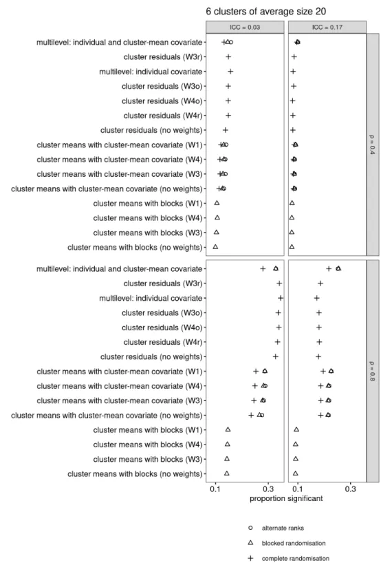
5.2.1 Six small clusters

With six clusters of average size 20, all analyses have abysmal power to detect a treatment effect of 0.25 units (relative to a within-cluster variance of 1 unit and a between-cluster variance that depends on the unconditional ICC). As shown in Figure 9 on page 33, it seems that the relative best approach across the ICC and ρ combinations is to assign the clusters in an alternate rank design (ARD) or in a blocked randomised design (BRD) and then include both the individual and cluster mean covariate scores as predictors in a

(32)

multilevel model. This method has only slightly worse power than some alternatives when the ICC is low and the covariate is highly informative (bottom left panel), but otherwise performs on par with the alternatives or outperforms them.

When an ARD or BRD design is not possible, the multilevel model also compares favourably to the alternatives when the ICC is fairly high; when the ICC is fairly low, other analyses, such as an analysis on the cluster mean residualised outcomes weighted by the inverse of the theoretical estimated variance of the cluster mean residualised outcomes (W3r, r for residuals), may be preferable.

5.2.2 Six large clusters

With six clusters of average size 200, the assignment methods that take the covariate into account (ARD, BRD) combined with one of the ancovas on the cluster means work best for all four combinations of parameters that would be unknown (ICC, ρ), as shown in Figure 10 on page 34. The multilevel model with both individual and cluster mean covariate scores performs similarly well.

When the assignment method cannot take the covariate into account and a completely randomised design is the only option, these analytic strategies still compare favourable to the other strategies. For reference, with ICC = 0.03 and ρ = 0.8, an ancova on an ARD or BRD study has about 93–95% power, whereas an ancova on a CRD study has about 87–89% power.

5.2.3 Twelve small clusters

With twelve clusters of average size 20, all analytic options have poor power when the covariate is weakly informative (ρ = 0.4): depending on the ICC, their power hovers around 0.15 and 0.30–0.35; see Figure 11 on page 35. Among these weakly performing options, the ARD and BRD designs coupled with one of the ancovas on the cluster means and the multilevel model with both individual and cluster-mean covariate scores represent the relative most powerful subset. These models still compare favourably to the other options when the study adopts a completely randomised design, though they are not uniformly more powerful across the two ICC parameter settings.

When a more informative covariate is available (ρ = 0.8), decent power levels can be achieved. Across the two ICC parameter settings, ARD and BRD designs coupled with one of the ancovas or the multilevel model are ever so slightly more powerful than CRD designs coupled with ancovas. The latter

(33)

Figure 9: Observed power of several assignment/analysis combinations when the sample consists of six clusters of average size 20. Only the assignment/analysis combinations whose Type-I error rate is acceptable are shown.

(34)

(35)

Figure 11: Observed power of several assignment/analysis combinations when the sample consists of twelve clusters of average size 20. Only the assignment/analysis combinations whose Type-I error rate is acceptable are shown.

(36)

in turn outperform CRDs coupled with an analysis on cluster mean residuals by a considerable margin for large ICCs, but are somewhat less powerful for small ICCs.

5.2.4 Twelve large clusters

With twelve clusters of average size 200, any of the three assignment methods (ARD, BRD, CRD) coupled with an ancova on the cluster means or a multi-level model with both individual and cluster mean covariate scores performs at least on par with the other approaches and blows them out of the water for some parameter combinations; see Figure 12. When the covariate is weakly informative, slightly more power can be obtained when adopting an ARD or BRD; when the covariate is more informative, any assignment method virtually guarantees perfect power.

5.2.5 Thirty-six small clusters

With 36 clusters of average size 20, any of the three assignment methods (ARD, BRD, CRD) coupled with an ancova on the cluster means or a multilevel model with both the individual and cluster mean covariate scores performs at least on par with the other approaches across all parameter combinations; see Figure 13 on page 38.

5.2.6 Thirty-six large clusters

With 36 clusters of average size 200, any of the three assignment methods (ARD, BRD, CRD) coupled with any analysis method save for the analyses on the cluster mean residualised outcomes or the multilevel model with only individual covariate scores virtually guarantees perfect power across all parameter combinations; see Figure 14 on page 39.

5.3 Adjusted power

In the previous subsection, an analytic approach’s power was estimated as the proportion of datasets generated for a given combination of simulation parameters on which this approach obtained a significant result (i.e., a p-value lower than 0.05). An alternative way to compute power, however, is to proceed as follows.

First, look up the fifth percentile of the p-values obtained by this analytic approach for the combination of simulation parameters of interested when the intervention effect was fixed at 0. Consider, for instance, the unweighted ancova on cluster means ran on a completely randomised design for six

(37)

(38)

Figure 13: Observed power of several assignment/analysis combinations when the sample consists of 36 clusters of average size 20. Only the as-signment/analysis combinations whose Type-I error rate is acceptable are shown.

(39)

Figure 14: Observed power of several assignment/analysis combinations when the sample consists of 36 clusters of average size 200. Only the assignment/analysis combinations whose Type-I error rate is acceptable are shown.

(40)

clusters of average size 20 with ρ = 0.4 and ICC = 0.03. The fifth percentile of the p-values obtained by this analysis on this combination of simulation parameters when the intervention effect was fixed at 0 was 0.047, i.e., 5% of the p-values were lower than 0.047. In principle, this 5th percentile should be 0.05, but due to chance, minor deviations are possible.

Second, for the power estimate, compute how often this analytic approach for this combination of simulation parameters yielded a p-value lower than the fifth percentile figure obtained in the first step. Call this proportion the estimated adjusted power. In our example, the analytic approach yields p < 0.05 on 11.4% of the datasets. But it only ‘beats’ its own Type-I error (i.e., p < 0.047) on 10.8% of the datasets.

The figures in the previous subsection show the first type of estimate (11.4% in the example), but these estimates may be slightly too optimistic (if the approach’s Type-I error was slightly larger than 5%) or too pessimistic (if its Type-I error was slightly smaller than 5%). The adjusted power estimates (10.8% in our example) should correct for such optimism or pessimism. I will not present the results for the adjusted power estimates in full (but see https://osf.io/wzjra/); the following observations suffice.

• For 6 clusters of average size 20, the multilevel model with both individ-ual and cluster mean covariate scores applied to an ARD or BRD still strikes the best balance across the simulation parameters. When only a CRD is possible, this analytic approach ranks among the most powerful alternatives. That said, power is dreadful overall for such small studies. • For all other sample sizes, the results for the adjusted power estimates

corroborate those for the ‘naive’ power estimates.

6 Discussion and conclusion

The central finding of this series of simulations is that ancovas ran on cluster mean outcomes with the cluster mean covariate scores as a predictor and multilevel models with both individual and cluster-mean covariate scores as predictors tend to yield most power when analysing cluster-randomised experiments while still retaining their nominal Type-I error rate. A slight increase in power can further be obtained when the clusters are assigned to the conditions in an alternate ranks or blocked randomised design rather than in a completely randomised design. When only a handful of small clusters are available for the experiment, power will probably be dreadful, even when a highly informative pre-treatment covariate is available.

(41)

The anovas with close-to-nominal Type-I error rates either did not use regression weights or they used cluster sizes (W1), estimated ‘theoretical’ cluster mean variances (W3) or the ratios of the cluster sizes over their design effect (W4) as weights. The differences among these were minute in these simulations, but it bears pointing out that the cluster sizes only varied over a restricted range. This stems from my motivation for running these simulations: to give advice to students and colleagues whose research is class- or school-based. I invite researchers who anticipate to work with clusters that vary more considerably in size to run their own simulations using the scripts available at https://osf.io/wzjra/ in order to find out which analytic method optimises power while retaining its nominal Type-I error. For instance, when a couple of the clusters are very large but most are fairly small, such simulations would show that the ancova with cluster sizes as weights is slightly anticonservative.

Similarly, I only simulated studies that assigned half of the clusters to each condition. Researchers who anticipate an unbalanced distribution of clusters over conditions are invited to adapt my scripts and run their own simulations. Lastly, the restricted scope of these simulations bears pointing out:

1. They assume that the pre-treatment covariate is linearly related to the outcome. I think this is a reasonable assumption since the covariate will typically be some pretest score, and pretest and posttest scores tend to be linearly related. But floor and ceiling effects in the covariate or the outcome may throw a spanner in the works.

2. They assume that there is no interaction between the pre-treatment covariate and the experimental condition. That is, participants with low covariate scores do not tend to profit more from the intervention than participants with high covariate scores or vice versa. Whether this assumption is approximately reasonable, will depend on the specifics of the study.

3. They assume that there is no heterogeneity between the clusters in terms of the intervention effect (i.e., all classes in the intervention condition profit equally from the intervention effect) and in terms of the informativeness of the covariate.

4. The covariate scores within each cluster were drawn from normal dis-tributions, and the differences between classes were, too. The alternate ranks and blocked randomised designs performed more or less equally well in these simulations; it is possible that the alternate ranks design will outperform the blocked randomised design when the covariate scores stem from a skewed distribution.

(42)

With these caveats in mind, I tentatively proffer the following advice to researchers planning cluster-randomised experiments:

1. Reconsider if you will only be able to recruit a small number of small clusters.

2. Try to obtain a good measure of the participants’ performance before the intervention, e.g., a pretest score of some sort.

3. If feasible, compute the mean covariate score per cluster and assign the clusters to conditions on the basis of this information (ARD or BRD). If not, don’t fret—the loss of power incurred is likely small.

4. For the analysis, either run a straightforward ancova on the cluster mean outcomes using the cluster mean covariate scores as your covariate or fit the individual data in a multilevel model using both the individual covariate scores and the cluster mean covariate scores as covariates. Personally, I would opt for the ancova without weighting or using clusters sizes as weights because of its simplicity.

Software used

R Core Team (2020); Bates et al. (2020); Bates et al. (2015); Kuznetsova, Bruun Brockhoff & Haubo Bojesen Christensen (2020); Kuznetsova, Brockhoff & Christensen (2017); Hothorn et al. (2019); Zeileis & Lumley (2019); Wickham (2019); Wickham et al. (2019); Zeileis (2006).

References

Barcikowski, Robert S. 1981. Statistical power with group mean as the unit of analysis. Journal of Educational Statistics 6(3). 267–285. doi:10.2307/1164877. Bates, Douglas, Martin Maechler, Ben Bolker & Steven Walker. 2020. Lme4: Linear mixed-effects models using ’eigen’ and s4. https://CRAN.R-project. org/package=lme4.

Bates, Douglas, Martin Mächler, Ben Bolker & Steve Walker. 2015. Fitting linear mixed-effects models using lme4. Journal of Statistical Software 67(1). 1–48. doi:10.18637/jss.v067.i01.

Bland, J. Martin & Sally M. Kerry. 1998. Weighted comparison of means. BMJ 316(7125). 129. doi:10.1136/bmj.316.7125.129.

(43)

Using covariates to improve precision for studies that randomize schools to evaluate educational interventions. Educational Evaluation and Policy Analysis 29(1). 30–59. doi:10.3102/0162373707299550.

Campbell, Michael J. & Stephen J. Walters. 2014. How to design, analyse and report cluster randomised trials in medicine and health related research. Chichester, UK: Wiley.

Dalton, Starrett & John E. Overall. 1977. Nonrandom assignment in AN-COVA: The alternate ranks design. Journal of Experimental Education 46(1). 58–62. doi:10.1080/00220973.1977.11011611.

Faraway, Julian J. 2005. Linear models with R. Boca Raton, FL: Chapman & Hall/CRC.

Faraway, Julian J. 2006. Extending the linear model with r: Generalized linear, mixed effects and nonparametric regression models. Boca Raton, FL: Chapman & Hall/CRC.

Hayes, Richard J. & Lawrence H. Moulton. 2009. Cluster randomised trials. Boca Raton, FL: Chapman & Hall/CRC.

Hedges, Larry V. 2007. Correcting a significance test for cluster-ing. Journal of Educational and Behavioral Statistics 32(2). 151–179. doi:10.3102/1076998606298040.

Hedges, Larry V. & E. C. Hedberg. 2007. Intraclass correlation values for planning group-randomized trials in education. Educational Evaluation and Policy Analysis 29(1). 60–87. doi:10.3102/0162373707299706.

Hothorn, Torsten, Achim Zeileis, Richard W. Farebrother & Clint Cummins. 2019. Lmtest: Testing linear regression models. https://CRAN.R-project.org/ package=lmtest.

Johnson, Jacqueline L., Sarah M. Kreidler, Diane J. Catellier, David M. Murray, Keith E. Muller & Deborah H. Glueck. 2015. Recommendations for choosing an analysis method that controls Type I error for unbalanced cluster sample designs with Gaussian outcomes. Statistics in Medicine 34(27). 3531–3545. doi:10.1002/sim.6565.

Kerry, Sally M. & J. Martin Bland. 1998. Analysis of a trial randomised in clusters. BMJ 316. 54. doi:10.1136/bmj.316.7124.54.

(44)

Klar, Neil & Gerarda Darlington. 2004. Methods for modelling change in cluster randomization trials. Statistics in Medicine 23. 2341–2357. doi:10.1002/sim.1858.

Kuznetsova, Alexandra, Per B. Brockhoff & Rune H. B. Christensen. 2017. lmerTest package: Tests in linear mixed effects models. Journal of Statistical Software 82(13). 1–26. doi:10.18637/jss.v082.i13.

Kuznetsova, Alexandra, Per Bruun Brockhoff & Rune Haubo Bojesen Chris-tensen. 2020. LmerTest: Tests in linear mixed effects models. https://CRAN.R-project.org/package=lmerTest.

Maxwell, Scott E., Harold Delaney & Charles A. Hill. 1984. Another look at ANCOVA versus blocking. Psychological Bulletin 95(1). 136–147. doi:10.1037/0033-2909.95.1.136.

McAweeney, Mary J. & Alan J. Klockars. 1998. Maximizing power in skewed distributions: Analysis and assignment. Psychological Methods 3(1). 117– 122. doi:10.1037/1082-989X.3.1.117.

Moerbeek, Mirjam. 2006. Power and money in cluster randomized trials: When is it worth measuring a covariate? Statistics in Medicine 25(15). 2607–2617. doi:10.1002/sim.2297.

Murray, David M. & Jonathan L. Blitstein. 2003. Methods to reduce the impact of intraclass correlation in group-randomized trials. Evaluation Review 27(1). 79–103. doi:10.1177/0193841X02239019.

Raudenbusch, Stephen W., Andres Martinez & Jessaca Spybrook. 2007. Strategies for improving precision in group-randomized ex-periments. Educational Evaluation and Policy Analysis 29(1). 5–29. doi:10.3102/0162373707299460.

R Core Team. 2020. R: A language and environment for statistical computing. Vienna, Austria: R Foundation for Statistical Computing. https://www.R-project.org/.

Schochet, Peter Z. 2008. Statistical power for random assignment evaluations of education programs. Journal of Educational and Behavioral Statistics 33(1). 62–87. doi:10.3102/1076998607302714.