Evaluation of black carbon estimations in global aerosol models

HAL Id: hal-02870410

https://hal.archives-ouvertes.fr/hal-02870410

Submitted on 16 Jun 2020

HAL is a multi-disciplinary open access

archive for the deposit and dissemination of

sci-entific research documents, whether they are

pub-lished or not. The documents may come from

teaching and research institutions in France or

abroad, or from public or private research centers.

L’archive ouverte pluridisciplinaire HAL, est

destinée au dépôt et à la diffusion de documents

scientifiques de niveau recherche, publiés ou non,

émanant des établissements d’enseignement et de

recherche français ou étrangers, des laboratoires

publics ou privés.

models

D. Koch, M Schulz, S. Kinne, C. Mcnaughton, J. R. Spackman, Yves

Balkanski, S. Bauer, T. Berntsen, T. Bond, O. Boucher, et al.

To cite this version:

D. Koch, M Schulz, S. Kinne, C. Mcnaughton, J. R. Spackman, et al.. Evaluation of black carbon

estimations in global aerosol models. Atmospheric Chemistry and Physics, European Geosciences

Union, 2009, 9 (22), pp.9001-9026. �10.5194/acp-9-9001-2009�. �hal-02870410�

© Author(s) 2009. This work is distributed under the Creative Commons Attribution 3.0 License.

Chemistry

and Physics

Evaluation of black carbon estimations in global aerosol models

T. Iversen13,27, A. Kirkev˚ag27, Z. Klimont7, Y. Kondo11, M. Krol12, X. Liu23,18, R. Miller2, V. Montanaro24, N. Moteki11, G. Myhre13,28, J. E. Penner23, J. Perlwitz1,2, G. Pitari24, S. Reddy14, L. Sahu11, H. Sakamoto11,

G. Schuster5, J. P. Schwarz9, Ø. Seland27, P. Stier25, N. Takegawa11, T. Takemura26, C. Textor3, J. A. van Aardenne8, and Y. Zhao21

1_{Columbia University, New York, NY, USA} 2_{NASA GISS, New York, NY, USA}

3_{Laboratoire des Sciences du Climat et de l’Environnement, Gif-sur-Yvette, France} 4_{Max-Planck-Institut fur Meteorologie, Hamburg, Germany}

5_{NASA Langley Research Center, Hampton, Virginia, USA} 6_{University of Illinois at Urbana-Champaign, Urbana, IL, USA}

7_{International Institute for Applied Systems Analysis, Laxenburg, Austria}

8_{European Commission, Institute for Environment and Sustainability, Joint Research Centre, Ispra, Italy}

9_{NOAA Earth System Research Laboratory, Chemical Sciences Division and Cooperative Institute for Research in}

Environmental Sciences, University of Colorado, Boulder, Colorado, USA

10_{University of Hawaii at Manoa, Honolulu, Hawaii, USA} 11_{RCAST, University of Tokyo, Japan}

12_{Meteorology and Air Quality, Wageningen University, Wageningen, The Netherlands} 13_{University of Oslo, Oslo, Norway}

14_{Universite des Sciences et Technologies de Lille, CNRS, Villeneuve d’Ascq, France} 15_{NASA Goddard Space Flight Center, Greenbelt, MD, USA}

16_{EC, Joint Research Centre, Institute for Environment and Sustainability, Ispra, Italy} 17_{University of Maryland Baltimore County, Baltimore, Maryland, USA}

18_{Pacific Northwest National Laboratory, Richland, USA}

19_{NOAA, Geophysical Fluid Dynamics Laboratory, Princeton, New Jersey, USA} 20_{ARQM Meteorological Service Canada, Toronto, Canada}

21_{University of California – Davis, CA, USA} 22_{NCAR, Boulder, CO, USA}

23_{University of Michigan, Ann Arbor, MI, USA} 24_{Universita degli Studi L’Aquila, Italy}

25_{Atmospheric, Oceanic and Planetary Physics, University of Oxford, UK} 26_{Kyushu University, Fukuoka, Japan}

27_{Norwegian Meteorological Institute, Oslo, Norway}

28_{Center for International Climate and Environmental Research – Oslo (CICERO) Oslo, Norway}

Received: 1 July 2009 – Published in Atmos. Chem. Phys. Discuss.: 24 July 2009

Abstract. We evaluate black carbon (BC) model predictions

from the AeroCom model intercomparison project by con-sidering the diversity among year 2000 model simulations and comparing model predictions with available measure-ments. These model-measurement intercomparisons include BC surface and aircraft concentrations, aerosol absorption optical depth (AAOD) retrievals from AERONET and Ozone Monitoring Instrument (OMI) and BC column estimations based on AERONET. In regions other than Asia, most mod-els are biased high compared to surface concentration mea-surements. However compared with (column) AAOD or BC burden retreivals, the models are generally biased low. The average ratio of model to retrieved AAOD is less than 0.7 in South American and 0.6 in African biomass burning re-gions; both of these regions lack surface concentration mea-surements. In Asia the average model to observed ratio is 0.7 for AAOD and 0.5 for BC surface concentrations. Com-pared with aircraft measurements over the Americas at lati-tudes between 0 and 50N, the average model is a factor of 8 larger than observed, and most models exceed the mea-sured BC standard deviation in the mid to upper troposphere. At higher latitudes the average model to aircraft BC ratio is 0.4 and models underestimate the observed BC loading in the lower and middle troposphere associated with springtime Arctic haze. Low model bias for AAOD but overestimation of surface and upper atmospheric BC concentrations at lower latitudes suggests that most models are underestimating BC absorption and should improve estimates for refractive in-dex, particle size, and optical effects of BC coating. Retrieval uncertainties and/or differences with model diagnostic treat-ment may also contribute to the model-measuretreat-ment dispar-ity. Largest AeroCom model diversity occurred in northern Eurasia and the remote Arctic, regions influenced by anthro-pogenic sources. Changing emissions, aging, removal, or optical properties within a single model generated a smaller change in model predictions than the range represented by the full set of AeroCom models. Upper tropospheric con-centrations of BC mass from the aircraft measurements are suggested to provide a unique new benchmark to test scav-enging and vertical dispersion of BC in global models.

1 Introduction

Black carbon, the strongly light-absorbing portion of car-bonaceous aerosols, is thought to contribute to global warm-ing since pre-industrial times. It is a product of incom-plete combustion of fossil fuels and biofuels, such as coal, wood and diesel. Black carbon (BC) has several effects on climate, primarily warming, but potentially also some amount of cooling. The “direct effect” is the scattering

Correspondence to: D. Koch

(dkoch@giss.nasa.gov)

and absorption of incoming solar radiation by the BC sus-pended in the atmosphere. The absorption warms the air where the BC aerosol is suspended, but the extinction of radiation results in negative forcing at the earth’s surface (e.g. Ramanathan and Carmichael, 2008). The “BC-albedo effect” occurs because black carbon deposited on snow low-ers the snow albedo and may therefore promote snow and ice melting (e.g. Warren and Wiscombe, 1980; Hansen and Nazarenko, 2004). BC may also have important effects on clouds by changing atmospheric stability and/or relative hu-midity, and thus affect cloud formation; this has been termed the “semi-direct effect” (e.g. Ackerman et al., 2000; Johnson et al., 2004). Finally, BC is a primary aerosol particle and influences the number of particles available for cloud con-densation (e.g. Oshima et al., 2009); it may thus play an im-portant role for the aerosol cloud “indirect effect”. BC may also affect the indirect effect by acting as ice nuclei (e.g. Co-zic et al., 2007; Liu et al., 2009).

Quantifying the effects of black carbon on climate change is hindered by several uncertainties. Emissions are uncertain because of difficulties quantifying sources and emission fac-tors (e.g. Bond et al., 2004). Measurements of BC concentra-tions are uncertain because of instrumental limitaconcentra-tions in the present measurement techniques (Andreae and Gelencser, 2006). Optical properties are uncertain since these vary with source, morphology, particle age and chemical processing. Atmospheric column aerosol absorption comes mostly from black carbon in many polluted and biomass burning regions. This absorption aerosol optical depth (AAOD) has been re-trieved from satellite and an array of sunphotometer mea-surements, and these retrievals also help to constrain column BC. However the constraint is limited by uncertainties and assumptions in the retrievals as well as by the fact that other absorbing species besides BC are present, such as dust and organic carbon. Model simulation of BC is complicated by uncertainties in treatment of initial particle size and shape ap-propriate for initial release in a model gridbox, particle up-take in liquid or frozen clouds and precipitation, treatment of mixing state and optical properties. Assumptions influencing the degree of internal vs. external mixing with water-soluble particles in the accumulation mode strongly influence the aerosol absorption (Seland et al., 2008) and CCN-activation. Internal mixing of BC also affects BC lifetime, decreasing it relative to hydrophobic BC (Ogren and Charlson, 1983; Stier et al., 2006, 2007). Furthermore, the BC model predictions are subject to model uncertainties that apply to any chemical model simulation, such as the accuracy of the model’s meteo-rology including transport, clouds, and precipitation (e.g. Liu et al., 2007).

The aim of this study is to evaluate model-calculated BC in recent state-of-the-art global models with aerosol chem-istry and physics, to consider their diversity and compare them with available observations. There has been concern that some models may greatly underestimate BC absorption and therefore BC contribution to climate warming (e.g. Sato

et al., 2003; Ramanathan and Carmichael, 2008; Seland et al., 2008). However it is unclear whether this is a problem common to all models, whether the problem is regional or global, and the extent to which the bias is due to BC mass underestimation possibly linked to emissions underestima-tion, or to model treatment of optical properties leading to underestimation of BC absorption. We examine these issues by comparing the models to a variety of measurements, and working with a large number of current models. We also in-vestigate whether biases in some regions are more problem-atic than in others. Finally we make use of one of the models, the GISS model (available to the first author of this paper), to consider the effects of changing BC emissions, aging, re-moval assumptions and optical properties. We also use the GISS model to consider the seasonality of model bias and the spectral dependence of AAOD bias.

We compare the models with several types of observa-tions. Model surface concentrations are compared with long-term surface concentration measurements. Model BC con-centration profiles are compared with aircraft measurements for several recent aircraft campaigns, spanning the North American region from the tropics to the Arctic. Column BC is assessed by comparing model AAOD with that re-trieved by Dubovik and Kings (2000) inversion algorithm from AERONET sunphotometer measurements (Holben et al., 1998), as was done in Sato et al. (2003), and with OMI satellite retrievals of AAOD. We also compare column bur-den of BC with the AERONET-based estimation as in Schus-ter et al. (2005). While the measurements provide constraints for the models, in the final section we will discuss measure-ment uncertainties and the discrepancies among them that are apparent as we apply them to the models.

2 Model descriptions 2.1 AeroCom models

We evaluate seventeen models from the AeroCom aerosol model intercomparison, an exercise that has been ongoing for the past 5 years. Model results, as well as observa-tion datasets for validaobserva-tion purposes, are available at the Ae-roCom website (http://nansen.ipsl.jussieu.fr/AEROCOM/). The AeroCom intercomparison exercises included an exer-cise “A” with each model using its own emissions, and an exercise “B” where all models used identical emissions, and were described in detail in Textor et al. (2006, 2007), Kinne et al. (2006) and Schulz et al. (2006). Here we work with exercise A unless only B is available for a particular model in the database. The models used year 2000 emissions and in some cases year 2000 meteorological fields. Not all di-agnostics were available for all models, so we used all those available for each quantity considered. Many aspects of the models have been evaluated in previous publications, and we refer to those for general background information. Textor et

al. (2006) provided a first comparison of the models in ex-periment A and included basic information on the models such as model resolution, chemistry, and removal assump-tions. Textor et al. (2007) described the exercise B model intercomparison, and showed that model diversity was not greatly reduced by unifying emissions, indicating that the greatest model differences result from features such as me-teorology and aerosol treatments rather than from emissions. Kinne et al. (2006) discussed the aerosol optical properties of the models and Schulz et al. (2006) presented the radiative forcing estimates for the models.

Some of the model features most relevant for the BC sim-ulations are provided in Table 1. As shown there, nine dif-ferent BC energy emissions inventories and eleven difdif-ferent biomass burning emissions inventories were used. The mod-els had a variety of schemes to determine black carbon aging from a fresh to aged particle, where aged particles may be activated into cloud water. Ten models assumed that black carbon aged from hydrophobic to hydrophilic after a fixed lifetime; five models had microphysical mixing schemes to make the particles hydrophilic, in one model the black and organic carbon are assumed to be mixed when emitted, and one model had fixed solubility. In three cases the particle mixing affected optical/radiative properties. A variety of assumptions were made about how frozen clouds removed aerosols compared to liquid clouds, ranging from identical treatments for frozen and liquid clouds to zero removal by ice clouds. Black carbon lifetime ranges from 4.9 to 11.4 days.

We note that the model versions evaluated here were sub-mitted to the database in year 2005, and many models have evolved significantly since (e.g. Bauer et al., 2008; Chin et al., 2009; Ghan and Zaveri, 2007; Liu et al., 2005, 2007; Myhre et al., 2009; Stier et al., 2006, 2007; Takemura et al., 2009). Thus this study provides a benchmark at the time of the 2005 submission.

2.2 GISS model sensitivity studies

We use the GISS aerosol model to study sensitivity to fac-tors that could impact the BC simulation. The GISS aerosol scheme used here includes mass of sulfate, sea-salt (Koch et al., 2006), carbonaceous aerosols (Koch et al., 2007) and dust (Miller et al., 2006; Cakmur et al., 2006). The sensitiv-ity studies are described below and listed in Table 2. All simulations are performed and averaged for 3 years, after a 2-year model spin-up. The standard GISS model version for these sensitivity studies is slightly different than the ver-sion in the AeroCom database. This verver-sion does not include dust-nitrate interaction, and does not include enhanced re-moval of BC by precipitating convective clouds as was in-cluded in the AeroCom-database GISS model version, and therefore has a somewhat larger BC load.

Table 1. AeroCom model black carbon characteristics.

AeroCom models Energy BB Emis(1) _Aging(2) _{BC Ice/snow Mass median BC Refractive MABS References for aerosol module}

Emis(1) _{lifetime removal}(3) _{diameter of density index at m}2_g−1(5,6)

days emitted g cm−3(6) 550 nm(6) particle(4)

GISS 99 B04 GFED A 7.2 12% 0.08 1.6 1.56–0.5i 8.4 Koch et al. (2006, 2007), Miller et al. (2006) ARQM 99 C99 L00, I 6.7 T 0.1 1.5 4.1 Zhang et al. (2001);

L96 Gong et al. (2003)

CAM C99 L96 A L X X X Collins et al. (2006)

DLR CW96 CW96 I 5% 0.08, 0.75 FF X X X Ackermann et al. (1998) accum, 0.02,

strat 0.37 BB

GOCART C99 GFED, A 6.6 T 0.078 1.0 1.75–0.45i 10.0 Chin et al. (2000, 2002),

D03 Ginoux et al. (2001)

SPRINTARS NK06 NK06 BCOC L 0.0695 FF, 1.25 1.75–0.44i 2.3 Takemura et al. (2000, 2002,

0.1 others 2005)

LOA B B04 GFED A 7.3 LI 0.0118 1.0 1.75–0.45i 8.0 # Boucher and Anderson (1995); Boucher et al. (2002); Reddy and Boucher (2004); Guibert et al. (2005) LSCE G03 G03 A 7.5 L 0.14 1.6 1.75-0.44i 3.5 Claquin et al. (1998, 1999);

(4.4 #) Guelle et al. (1998a, b, 2000); Smith and Harrison (1998); Balkanski et al. (2003); Bauer et al. (2004); Schulz et al. (2006) MATCH L96 L96 A L 0.1 X X X Barth et al. (2000);

Rasch et al. (2000, 2001) MOZGN C99, M92 A L 0.1 1.0 1.75–0.44i 8.7 Tie et al. (2001, 2005)

O96

MPIHAM D06 D06 I # 4.9 S 0.069 (FF, BF) 2.0 1.75–0.44i 7.7 # Stier et al. (2005) 0.172 (BB)

MIRAGE C99 CW96, I # 6.1 L 0.19, 0.025 1.7 1.9-0.6i 3 aitk, Ghan et al. (2001); Easter et al. L00 6 acc (2004); Ghan and Easter (2006) TM5 D06 D06 A 5.7 20% 0.034 1.6 1.75-0.44i 4.3 Metzger et al. (2002a, b) UIOCTM C99 CW96 A 5.5 L 0.1 (FF), 1.0 1.55-0.44i 7.2 # Grini et al. (2005); Myhre et al.

0.295, (2003); Berglen et al. (2004); 0.852 (BB) Berntsen et al. (2006) UIOGCM 99 IPCC IPCC I # 5.5 none 0.0236–0.4 2.0 2.0–1.0i 10.5 # Iversen and Seland (2002);

Kirkevag and Iversen (2002); Kirkevag et al. (2005) UMI L96 P93 N 5.8 L 0.1452 (FF), 1.5 1.80–0.5i 6.8 # Liu and Penner (2002)

0.137 (BB)

ULAQ 99 IPCC IPCC A 11.4 L 0.02–0.32 1.0 2.07–0.6i 7.5 # Pitari et al. (1993, 2002) (1)_{BB = biomass burning; B04 = Bond et al. (2004); C99 = Cooke et al. (1999); L00 = Lavoue et al. (2000); L96 = Liouse et al. (1996); CW} = Cooke and Wilson (1996); GFED = Van der Werf et al. (2003); NK06 = Nozawa and Kurokawa (2006); G03 = Generoso et al. (2003); R05 = Reddy et al. (2005); D03 = Duncan et al. (2003); D06 = Dentener et al. (2006); M92 = Mueller (1992); O96 = Olivier et al. (1996); IPCC = IPCC-TAR (2000); P93 = Penner et al. (1993)

(2)_{Aging as it affects particle solubility. A= aging with time; I= aging by coagulation and condensation, particles are internally mixed;} BCOC = BC assumed mixed with OC; N= none; # indicates that mixing/aging also affects particle optical properties.

(3)_{T= Temp dependence, L= as liquid, LI = As liquid for in-cloud removal only; S= Stier et al. (2005); % is relative to water.}

(4)_{FF = fossil fuel}

(5)_{MABS = BC mass absorption coefficient at 550 nm; # taken from Schulz et al. (2006).}

(6)_{X: models did not simulate optical properties.}

Table 2. GISS model sensitivity studies.

Description Emission Burden Lifetime, d AAOD x100

Tg yr−1 mg m−2 550 nm

Standard run, 7.2 (4.4 energy, 0.36 9.2 0.55

see text 2.8 biomass

burning) EDGAR32 7.5 0.37 9.3 0.58 emission IIASA emission 8.1 0.41 9.5 0.60 BB 1998 8.2 0.38 8.7 0.58 2x 7.2 0.29 7.6 0.50 (Faster aging) 2x 7.2 0.51 13 0.67 (Slower aging) 2x More ice-out 7.2 0.33 8.5 0.52 2x Less ice-out 7.2 0.38 9.8 0.57 Reff =0.1 µm 7.2 0.35 9.1 0.47 Reff =0.06 µm 7.2 0.36 9.3 0.70 2.2.1 Emissions

The standard GISS model uses carbonaceous aerosol energy production emissions from Bond et al. (2004). Biomass burning emissions are based on the Global Fire Emissions Database (GFED) v2 model carbon estimates for the years 1997–2006 (van der Werf et al., 2003, 2004), with the car-bonaceous aerosol emission factors from Andreae and Mer-let (2001). One sensitivity case had fossil and biofuel emis-sions from the Emission Database for Atmospheric Research (EDGAR V32FT2000, called “EDGAR32” below; Olivier et al., 2005) combined with emission factors from Bond et al. (2004) and in a second those of the International Institute for Applied Systems Analysis (IIASA) (Cofala et al., 2007). In a third we used the largest biomass burning year from the GFED dataset, 1998.

2.2.2 Aging and removal

In the standard GISS model, energy-related BC is assumed to be hydrophobic initially and then ages to become hydrophilic with an e-fold lifetime of 1 day. Biomass burning BC is as-sumed to have 60% solubility, so that if a cloud is present, 60% these aerosols are taken into the cloud water for each half-hour cloud timestep. One sensitivity test assigned a shorter lifetime with a halved e-folding time for energy BC and 80% solubility for biomass burning. A second test as-sumes a longer lifetime, with doubled e-folding time for en-ergy BC and 40% solubility for biomass burning.

Treatment of BC solubility is particularly uncertain for frozen clouds. In our standard model, BC-cloud uptake for frozen clouds is 12% of that for liquid clouds. A sensitivity run allowed 24% ice-cloud BC uptake, and another case 5%.

2.2.3 Aerosol size

The standard GISS model assumes the BC effective radius (cross section weighted radius over the size distribution; Hansen and Travis, 1974) is 0.08 µm. One sensitivity case increased this to 0.1µm, and another decreased it to 0.06 µm. The size primarily affects the BC optical properties. For BC sizes 0.1, 0.08 and 0.06 µm, the model global mean BC mass absorption efficiencies are 6.2, 8.4 and 12.4 and BC single scattering albedos are 0.31, 0.27 and 0.21.

3 Model evaluation 3.1 Surface concentrations

Annual average BC surface concentration measurements are shown in the first panel of Fig. 1. The data for the United States are from the IMPROVE network (1995–2001), those from Europe are from the EMEP network (2002–2003); some Asian data from 2006 are from Zhang et al. (2009); additional data, mostly from the late 1990s, are referenced in Koch et al. (2007). These data are primarily elemental car-bon, or refractory carcar-bon, which can be somewhat different than BC (Andreae and Gelencser, 2006). The data were not screened according to urban, rural or remote environment, all available data were used; however the IMPROVE sites are generally in rural or remote locations. There are broad re-gional tendencies, with largest concentrations in Asia (1000– 14 000 ng m−3), then Europe (500–5000 ng m−3), then the United States (100–500 ng m−3), then high northern latitudes (10–100 ng m−3) and least at remote locations (<10 ng m−3). Figure 1 also shows BC surface concentrations from the GISS model sensitivity studies. The biggest impact for

Observed BC surface concentration standard EDGAR

IIASA BB 1998 lifex2

life/2 ice/2 icex2

0 10 25 100 200 500 1000 5000 14500

Fig. 1. Observed BC surface concentrations (upper left panel) and GISS sensitivity model results (annual mean; ng m−3).

remote regions comes from increasing BC lifetime, either by doubling the aging rate or by reducing the removal by ice. Decreasing the BC lifetime has a smaller effect. The larger 1998 biomass burning emissions mostly increase BC in bo-real Northern Hemisphere and Mexico. EDGAR32 emis-sions increase BC in Europe, Arabia and northeastern Africa; IIASA emissions increase south Asian BC.

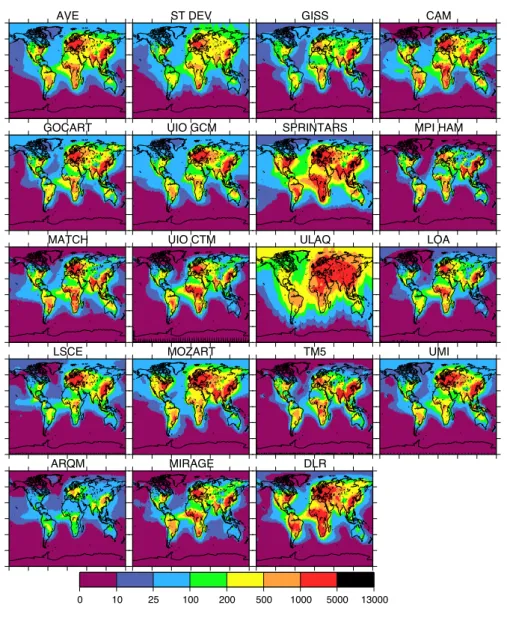
Figure 2 show the AeroCom model simulations of BC sur-face concentration, using model layer one from each model. Figure 2 also shows the average and standard deviations of the models. The standard deviation distribution is similar to the average. Regions of especially large model uncertainty occur where the standard deviation equals or exceeds the av-erage, such as the Arctic. Overall the models capture the observed distribution of BC “hot spots”. SPRINTARS is the only model that successfully captures the large BC concen-trations in Southeast Asia (Table 3), however it overestimates BC in other regions. Unfortunately there are no long-term measurements of BC in the Southern Hemisphere biomass burning regions.

Table 3 shows the ratio of modeled to observed BC in re-gions where surface concentration observations are available. The regional ratios are based on the ratio of annual mean model to annual mean observed for each site, averaged over

each region. Thirteen out of seventeen AeroCom models over-predict BC in Europe. Sixteen of the models underes-timate Southeast Asian BC surface concentrations; however most of these measurements are from 2004–2006 and emis-sions have probably increased significantly since the 1990s (Zhang et al., 2009). Nine of the models overestimate re-mote BC; in the United States about half the models over-estimate and half underover-estimate the observations. Overall, the models do not underestimate BC relative to surface mea-surements. None of the GISS model sensitivity studies show significant improvement over the standard case. The longer lifetime cases improve the model-measurement agreement in polluted regions but worsen the agreement in remote regions.

3.2 Aerosol absorption optical depth

The aerosol absorption optical depth (AAOD), or the non-scattering part of the aerosol optical depth, provides another test of model BC. AAOD is an atmospheric column measure of particle absorption, and so provides a different perspec-tive from the surface concentration measurements. Both BC and dust absorb radiation, so AAOD is most useful for test-ing BC in regions where its absorption dominates over dust absorption. Therefore we focus on regions where the dust

AVE ST DEV GISS CAM

GOCART UIO GCM SPRINTARS MPI HAM

MATCH UIO CTM ULAQ LOA

LSCE MOZART TM5 UMI

ARQM MIRAGE DLR

0 10 25 100 200 500 1000 5000 13000

Fig. 2. AeroCom models annual mean BC surface concentrations (ngm−3). First panel shows average, second panel shows standard deviation of models.

load is relatively small, for example Africa south of the Sa-hara Desert. However since some sites within these regions still have dust, we work with model total AAOD, including all species.

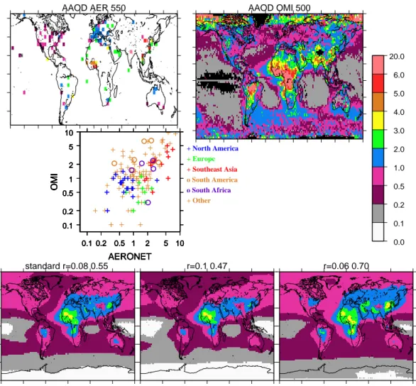
Figure 3 shows AERONET (1996–2006) sunphotometer (e.g. Dubovik et al., 2000; Dubovik and King, 2000) and OMI satellite (2005–2007, from OMAERUV product; Tor-res et al., 2007) retrievals of clear sky AAOD. A scatter plot compares the AERONET and OMI retrievals at the AERONET sites. Table 4 (last 5 rows) provides regional av-erage AAOD for these retrievals. The two retrievals broadly agree with one another. However, the OMI estimate is larger

than the AERONET value for South America and smaller for Europe and Southeast Asia.

The AeroCom model AAOD simulations are in Fig. 4. The standard deviation relative to the average is similar to the sur-face concentration result; it is less than or equal to the aver-age, except in parts of the Arctic. Table 4 gives the average ratio of model to retrieved AAOD within regions. For the ratio of model to AERONET we average the model AAOD over all AERONET sites within the region and divide by the average of the corresponding AERONET values. For OMI we average over each region in the model and divide by the OMI regional average. The average model agrees with the

Table 3. Average ratio between model and observed BC surface concentrations within regions for AeroCom models and GISS sen-sitivity studies. Number of measurements is given for each region. Bottom row is observed average concentration in ng m−3. Regions defined as N Am (130 W to 70 W; 20 N to 55 N), Europe (15 W to 45 E; 30 N to 70 N), Asia (100 E to 160 E; 20 N to 70 N).

AeroCom models N Am Europe Asia Rest of

#26 #16 #23 World #12 GISS 0.81 0.65 0.43 2.4 ARQM 0.29 0.49 0.12 0.55 CAM 1.6 2.2 0.40 1.8 DLR 3.0 3.1 0.37 1.4 GOCART 1.2 2.1 0.48 1.2 SPRINTARS 7.7 9.7 1.0 4.4 LOA 0.89 1.2 0.23 0.50 LSCE 0.61 3.0 0.43 0.81 MATCH 1.3 3.0 0.25 1.0 MIRAGE 1.2 1.7 0.32 0.76 MOZGN 2.4 3.8 0.76 2.2 MPIHAM 1.5 0.73 0.56 0.44 TM5 1.8 1.0 0.76 1.2 UIOCTM 0.72 1.6 0.37 0.41 UIOGCM 0.88 2.9 0.53 1.7 UMI 0.81 4.8 0.65 1.0 ULAQ 0.75 3.0 0.82 2.2 AeroCom Ave 1.6 2.6 0.50 1.4 AeroCom Median 1.2 2.2 0.43 1.2 GISS sensitivity std 0.81 0.88 0.42 1.9 r=.1 0.82 0.90 0.41 1.9 r=.06 0.82 0.91 0.42 2.0 EDGAR32 0.70 1.1 0.34 1.7 IIASA 0.70 0.86 0.50 1.9 BB1998 0.81 0.93 0.42 1.8 Lifex2 0.88 0.98 0.43 2.9 Life/2 0.78 0.80 0.38 1.5 Ice/2 0.83 0.93 0.41 2.1 Icex2 0.79 0.88 0.41 1.7 Observed (ng m−3) 290 1170 5880 750

retrievals in eastern North America and with AERONET in Europe (ratios of modeled to AERONET in these regions are 0.86 and 0.81); it underestimates Asian (ratio is 0.67) and biomass burning AAOD (about 0.5–0.7 for AERONET and 0.4–0.5 for OMI).

AAOD depends not just on aerosol load but also on op-tical properties, such as refractive index, particle size, den-sity and mixing state. In Fig. 3 we show how the GISS model AAOD changes with assumed effective radius. The global mean AAOD decreases/increases 15%/27% for an in-crease/decrease of 0.02 µm effective radius. Note that the

AeroCom model initial particle diameters (Table 1) span be-yond this range (0.01 to 0.9 µm) and in some cases grow as the particles age. Increasing particle density from 1.6 to 1.8 g cm−3in the GISS model decreases AAOD about as much as increasing particle size from 0.08 to 0.1 µm (calcu-lated but not shown). Thus the AAOD is highly sensitive to small changes in these optical properties.

Note that models generally underestimate AAOD but not surface concentration. As we will discuss below, this could result from inconsistencies in the measurements, from model under-prediction of BC aloft, or from under-prediction of ab-sorption. In this connection most models in the 2005-version of AeroCom did not properly describe internal mixing with scattering particles in the accumulation mode. Such mixing increases the absorption cross section of the aerosols com-pared to external mixtures of nucleation- and Aitken-mode BC particles.

3.3 Wavelength-dependence

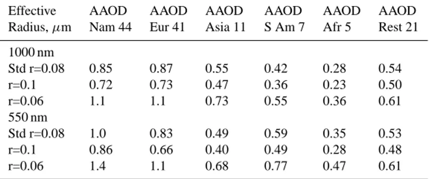
Black carbon absorption efficiency decreases less with in-creasing wavelength compared with dust or organic carbon (Bergstrom et al., 2007). Therefore comparison of AAOD with retrievals at longer wavelength indicates the extent to which BC is responsible for biases. In Fig. 5 we compare AERONET AAOD at 550 and 1000 nm with the GISS model AAOD for the wavelength intervals 300–770 nm and 860– 1250 nm respectively. Table 5 shows the ratio of the GISS model to AERONET within source regions for 1000 nm and 550 nm, for three different BC effective radii. In all regions except Europe and Asia, the ratio is even lower at the longer wavelength, confirming the need for increased simulated BC absorption, rather than other absorbing aerosols that absorb relatively less at longer wavelengths.

3.4 Seasonality

Our analysis has considered only annual mean observed and modeled BC. Here we present the seasonality of observed AAOD compared with the GISS model to explore how the bias may vary with season. Seasonal AAOD are shown for AERONET, OMI and the GISS model in Fig. 6. As in most of the models, the GISS model BC energy emis-sions do not include seasonal variation. Biomass burning emissions do, and dust seasonality is also very pronounced. However, transport and removal seasonal changes also cause fluctuations in model industrial source regions. Note that more AERONET data satisfy our inclusion criteria for the 3 month means compared with annual means (see figure cap-tions), so coverage is better in some regions and seasons than in the annual dataset in Fig. 3. Table 4 (bottom 4 rows) gives regional seasonal retrieved mean AAOD. The seasonal model-to-measurement ratios are also provided in the middle portion of Table 4.

AAOD AER 550 AAOD OMI 500 0.1 0.2 0.5 1 2 5 10 OMI 0.1 0.2 0.5 1 2 5 10 AERONET 0.1 0.2 0.5 1 2 5 10 OMI 0.1 0.2 0.5 1 2 5 10 AERONET 0.1 0.2 0.5 1 2 5 10 OMI 0.1 0.2 0.5 1 2 5 10 AERONET 0.1 0.2 0.5 1 2 5 10 OMI 0.1 0.2 0.5 1 2 5 10 AERONET 0.1 0.2 0.5 1 2 5 10 OMI 0.1 0.2 0.5 1 2 5 10 AERONET 0.1 0.2 0.5 1 2 5 10 OMI 0.1 0.2 0.5 1 2 5 10 AERONET + North America + Europe + Southeast Asia o South America o South Africa + Other standard r=0.08 0.55 r=0.1 0.47 r=0.06 0.70 0.0 0.1 0.2 0.5 1.0 2.0 3.0 4.0 5.0 6.0 20.0

Fig. 3. Top: Aerosol absorption optical depth, AAOD, (x100) from AERONET (at 550 nm; upper left), OMI (at 500 nm; upper right); middle: scatter plot comparing OMI and AERONET at AERONET sites; and bottom: GISS sensitivity studies for effective radius 0.08, 0.1, and 0.06 µm for 300–770 nm. The AERONET data are for 1996–2006, v2 level 2, annual averages for each year were used if >8 months were present, and monthly averages for >10 days of measurements. The values at 550 nm were determined using the 0.44 and 0.87 µm Angstrom parameters. The OMI retrieval is based on OMAERUVd.003 daily products from 2005–2007 that were obtained through and averaged using GIOVANNI (Acker and Leptoukh, 2007).

Biomass burning seasonality, with peaks in JJA for central Africa (OMI) and in SON for South America, is simulated in the model without clear change in bias with season. In Asia both retrievals have maximum AAOD in MAM, which the model underestimates (i.e. ratio of model to observed is low-est in MAM). The MAM peak may be from agricultural or biomass burning not underestimed by the model emissions. The other industrial regions do not have apparent seasonal-ity. However the model BC is underestimated most in Eu-rope during fall and winter suggesting excessive loss of BC or missing emissions during those seasons.

Summertime pollution outflow from North America seems to occur in both OMI and the model. The large OMI AAOD in the southern South Atlantic during MAM-JJA may be a retrieval artifact due to low sun-elevation angle and/or sparse sampling; however if it is real, then the model seasonality in this region is out of phase.

3.5 Column BC load

Model simulation of column BC mass (Fig. 7) in the atmo-sphere should be less diverse than the AAOD since it con-tains no assumptions about optical properties. However there is no direct measurement of BC load. Schuster et al. (2005) developed an algorithm to derive column BC mass from AERONET data, working with the non-dust AERONET cli-matologies defined by Dubovick et al. (2002). The Schuster algorithm uses the Maxwell Garnett effective medium ap-proximation to infer BC concentration and specific absorp-tion from the AERONET refractive index. The Maxwell Garnett approximation assumes homogeneous mixtures of small insoluble particles (BC) suspended in a solution of scattering material. Such mixing enhances the absorptivity of the BC. Schuster et al. (2005) estimated an average spe-cific absorption of about 10 m2g−1, a value larger than most

AVE ST DEV GISS GOCART

UIO GCM ARQM SPRINTARS MPI HAM

MIRAGE UIO CTM ULAQ LOA

LSCE MOZART TM5 UMI

0.0 0.1 0.2 0.5 1.0 2.0 3.0 4.0 5.0 6.0 20.0

Fig. 4. Annual average AAOD (x100) for AeroCom models at 550 nm. First panel is average, second panel standard deviation.

53 1216

Figure 5. Annual average AAOD (x100) at AERONET stations for 550 nm and 1000 nm (top 1217

left and right), and for the GISS model for 300-770nm (bottom left) and 860-1250nm (bottom 1218

right). 1219

Fig. 5. Annual average AAOD (x100) at AERONET stations for 550 nm and 1000 nm (top left and right), and for the GISS model for 300–770 nm (bottom left) and 860–1250 nm (bottom right).

Table 4. Average ratio of model to retrieved AERONET and OMI Aerosol Absorption Optical Depth at 550 nm within regions for AeroCom models and GISS sensitivity studies. Number of measurements is given for AERONET. Annual and seasonal measurement values are given in last 5 rows. Regions defined as N Am (130 W to 70 W; 20 N to 55 N), Europe (15 W to 45 E; 30 N to 70 N), Asia (100 E to 160 E; 30 N to 70 N), S Am (85 W to 40 W; 34 S to 2 S), Afr (20 W to 45 E; 34 S to 2 S).

AER AER AER AER AER AER OMI OMI OMI OMI OMI OMI

N Am Eur Asia S Am Afr Rest of N Am Eur Asia S Am Afr Rest of

#44 #41 #11 #7 #5 World #40 World GISS 1.0 0.83 0.49 0.59 0.35 0.88 0.73 1.4 0.74 0.29 0.40 0.28 ARQM 0.79 0.36 0.30 0.42 0.25 0.44 0.50 0.61 0.40 0.22 0.23 0.19 GOCART 1.4 1.5 1.4 0.72 0.79 0.96 0.79 2.5 1.4 0.34 0.72 0.46 SPRINTARS 1.4 0.48 0.44 1.8 1.2 0.64 0.76 0.69 0.59 0.83 1.3 0.28 LOA 0.57 0.56 0.42 0.44 0.70 0.44 0.32 0.95 0.44 0.25 0.48 0.18 LSCE 0.42 0.55 0.48 0.20 0.18 0.34 0.29 1.1 0.51 0.11 0.21 0.16 MOZGN 1.5 1.3 0.99 0.60 0.60 0.77 0.82 2.6 1.4 0.32 0.40 0.35 MPIHAM 0.39 0.21 0.29 0.43 0.35 0.21 0.21 0.29 0.32 0.22 0.35 0.082 MIRAGE 0.73 0.55 0.49 0.76 0.78 0.42 0.35 0.91 0.48 0.41 0.58 0.20 TM5 0.41 0.32 0.29 0.24 0.20 0.31 0.21 0.48 0.31 0.12 0.22 0.11 UIOCTM 0.62 0.67 0.46 1.1 0.61 0.57 0.37 1.1 0.53 0.57 0.54 0.19 UIOGCM 1.3 1.1 0.75 0.82 0.54 0.80 0.82 1.8 1.0 0.46 0.42 0.36 UMI 0.32 0.29 0.29 0.21 0.21 0.22 0.17 0.44 0.28 0.095 0.19 0.086 ULAQ 1.4 2.6 2.1 1.1 0.52 1.1 1.1 6.7 1.5 0.62 0.48 0.71 Ave 0.86 0.81 0.67 0.68 0.53 0.55 0.52 1.6 0.71 0.35 0.47 0.26 GISS sensitivity studies std 1.0 0.83 0.49 0.59 0.35 0.53 0.73 1.4 0.74 0.29 0.40 0.28 r=.1 0.86 0.66 0.40 0.49 0.28 0.48 0.60 1.2 0.61 0.24 0.32 0.22 r=.06 1.4 1.1 0.68 0.77 0.47 0.61 1.0 1.8 1.0 0.38 0.53 0.38 EDGAR32 1.1 0.81 0.46 0.57 0.35 0.58 0.75 1.4 0.73 0.28 0.41 0.29 IIASA 1.2 0.85 0.57 0.59 0.36 0.55 0.82 1.5 0.90 0.29 0.41 0.32 BB1998 1.1 0.81 0.51 0.67 0.40 0.55 0.80 1.4 0.84 0.31 0.45 0.30 Lifex2 1.3 0.91 0.54 0.66 0.41 0.58 0.93 1.6 0.88 0.35 0.50 0.39 Life/2 0.93 0.73 0.46 0.58 0.33 0.52 0.65 1.3 0.67 0.28 0.37 0.23 Ice/2 1.1 0.83 0.51 0.62 0.36 0.52 0.81 1.5 0.79 0.29 0.41 0.31 Icex2 0.96 0.74 0.48 0.58 0.34 0.52 0.68 1.3 0.71 0.31 0.39 0.24 Std DJF 0.85 0.45 0.45 0.29 0.33 0.31 0.40 0.40 0.64 0.22 0.30 0.36 Std MAM 0.96 0.86 0.51 0.41 0.38 0.46 0.95 1.2 0.60 0.21 0.33 0.38 Std JJA 0.83 0.97 0.64 0.43 0.30 0.66 0.63 1.7 0.93 0.28 0.36 0.36 Std SON 1.2 0.64 0.56 0.51 0.34 0.40 0.63 0.80 0.71 0.20 0.57 0.38 Retrieved x100 Annual 0.69 1.5 3.6 1.8 2.0 2.4 0.85 0.68 1.5 2.2 1.7 1.2 Average DJF 0.57 1.4 3.3 1.4 0.9 2.6 1.0 1.4 1.4 1.5 1.2 0.9 MAM 0.79 1.6 4.0 1.0 0.8 2.4 0.72 0.97 2.2 1.4 0.82 1.4 JJA 0.88 1.6 3.0 2.4 3.1 2.0 1.0 0.71 1.2 2.7 2.7 1.8 SON 0.57 1.6 3.0 3.1 3.9 2.2 0.95 1.0 1.4 4.7 1.4 1.1

of the models (see Table 1); however a lower value would in-crease the retrieved burden and worsen the comparison with the models.

An updated version of the AERONET-derived BC col-umn mass is shown in Figs. 7 and 8. For this retrieval, a BC refractive index of 1.95–0.79i was assumed, within the

range recommended by Bond and Bergstrom (2006), and BC density of 1.8 g cm−3. In the retrievals, most conti-nental regions have BC loadings between 1 and 5 mg m−2, with mean values for North America (1.8 mg m−2) and Europe (2.1 mg m−2) being somewhat smaller than Asia (3.0 mg m−2) and South America (2.7 mg m−2). The current

AAOD 550 DJF MAM JJA SON

OMI

model

0.0 0.1 0.2 0.5 1.0 2.0 3.0 4.0 5.0 6.0 20.0

Fig. 6. Seasonal average AAOD (x100) for AERONET 550 nm (top), OMI 500 nm (middle), standard GISS model 550 nm (bottom).

Table 5. The average ratio of GISS model to AERONET within regions for 1000 nm and 550 nm.

Effective AAOD AAOD AAOD AAOD AAOD AAOD

Radius, µm Nam 44 Eur 41 Asia 11 S Am 7 Afr 5 Rest 21 1000 nm Std r=0.08 0.85 0.87 0.55 0.42 0.28 0.54 r=0.1 0.72 0.73 0.47 0.36 0.23 0.50 r=0.06 1.1 1.1 0.73 0.55 0.36 0.61 550 nm Std r=0.08 1.0 0.83 0.49 0.59 0.35 0.53 r=0.1 0.86 0.66 0.40 0.49 0.28 0.48 r=0.06 1.4 1.1 0.68 0.77 0.47 0.61

industrial region retrievals are larger than the previous esti-mates of Schuster et al. (2005), which were 0.96 mg m−2for North America, 1.4 mg m−2for Europe and 1.6 mg m−2for Asia. The biomass burning estimates are similar to the previ-ous retrievals. The differences may be due to the larger span of years and sites in the current dataset.

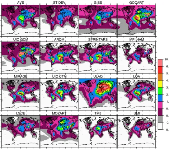
Figure 7 shows the AeroCom model BC column loads. The model standard deviation relative to the average is sim-ilar to the surface concentration (Fig. 2) and the AAOD (Fig. 4). The model column loads are smaller than the Schuster estimate. Some models agree quite well in Europe,

Southeast Asia or Africa (e.g. GOCART, SPRINTARS, MOZGN, LSCE, UMI). Model to retrieved ratios within re-gions are presented in Table 6. This ratio is generally smaller than model to retrieved AAOD in North America and Eu-rope. The inconsistencies among the retrievals would benefit from detailed comparison with a model that includes particle mixing and with model diagnostic treatment harmonized to the retrievals.

Figure 8 has GISS BC column sensitivity study re-sults. The load is affected differently than the surface concentrations (Fig. 1). The Asian IIASA emissions are

Schuster BC load _{AVE ST DEV GISS}

CAM GOCART UIO GCM ARQM

SPRINTARS MPI HAM MATCH MIRAGE

UIO CTM ULAQ LOA DLR

LSCE MOZART TM5 UMI

0.0 0.1 0.2 0.5 1.0 2.0 5.0 10.0 13.0

mg/m2

Fig. 7. Annual mean column BC load for 9 AeroCom models, mg m−2. The Schuster BC load is based on AERONET v2 level 1.5; annual averages require 12 months of data, data include all AERONET up to 2008.

larger than Bond (Bond et al., 2004) or EDGAR32, so that the outflow across the Pacific is greater. The large-biomass burning case (1998) also results in greater BC transport to Northwestern US in the column. Increasing BC lifetime in-creases both BC surface and column mass more than the other cases; however it has a larger impact on Southern Hemisphere load than surface concentrations. The reduced ice-out case has somewhat smaller impact on the column than at the surface, especially for some parts of the Arctic. The reduced ice-out thus has an enhanced effect at low levels, be-low ice-clouds, in the Arctic, while having a relatively small impact on the column. Modest model improvements relative

to the retrieval occur for the case with increased lifetime and for the IIASA emissions (Table 6).

3.6 Aircraft campaigns

We consider the BC model profiles in the vicinity of recent aircraft measurements in order to get a qualitative sense of how models perform in the mid-upper troposphere and to see how model diversity changes aloft. The measurements were made with three independent Single Particle Soot ab-sorption Photometers (SP2s) (Schwarz et al., 2006; Slowik et al., 2007) onboard NASA and NOAA research aircraft at tropical and middle latitudes (Fig. 9) and at high latitudes

standard 0.36 EDGAR 0.37 IIASA 0.41 BB 1998 0.38 lifex2 0.51 life/2 0.29 0.0 0.1 0.2 0.5 1.0 2.0 5.0 10.0 13.0 mg/m2

ice-out/2 0.38 ice-outx2 0.33 Schuster BC load

Fig. 8. Annual mean column BC load for GISS sensitivity simulations and the Schuster BC retrieval (see Fig. 7).

(Fig. 10) over North America. Details for the campaigns are provided in Table 7. The SP2 instrument uses an intense laser to heat the refractory component of individual aerosols in the fine (or accumulation) mode to vaporization. The de-tected thermal radiation is used to determine the black carbon mass of each particle (Schwarz et al., 2006). The U. Tokyo and the NOAA data have been adjusted 5–10% (70% dur-ing AVE-Houston) to account for the “tail” of the BC mass distribution that extends to sizes smaller than the SP2 lower limit of detection. This procedure has not been performed on the U. Hawaii data, however this instrument was config-ured to detect smaller particle sizes so that the unmeasconfig-ured mass is estimated to be less than about 13% (3% at smaller and 10% at larger sizes). The aircraft data in each panel of Figs. 9 and 10 are averaged into altitude bins along with standard deviations of the data. When available, data mean as well as median are shown. For cases in which signifi-cant biomass smoke was encountered (e.g. Figs. 9d, 10d and e), the median is more indicative of background conditions than the mean. However, for the spring ARCPAC campaign (Fig. 10c), four of the five flights encountered heavy smoke conditions, so in this case profiles are provided for the mean of the smoky flights and the mean for the remaining flight

which is more representative of background conditions. The ARCPAC NOAA WP-3D aircraft thus encountered heavier burning conditions (Fig. 10c; Warneke et al., 2009) than the other two aircraft for the Arctic spring (Fig. 10a and b).

Model profiles shown in each panel are constructed by averaging monthly mean model results at several locations along the flight tracks (map symbols in Figs. 9 and 10). We tested the accuracy of the model profile-construction ap-proach using the U. Tokyo data and the GISS model, by com-paring a profile constructed from following the flight tracks within the model fields with the simpler profile construction shown in Fig. 10a. The two approaches agreed very well except in the boundary layer (the lowest 1–2 model levels). Potentially more problematic is the comparison of instan-taneous observational snapshots to model monthly means. Nevertheless the comparison does suggest some broad ten-dencies.

The lower-latitude campaign observations (Fig. 9) indicate polluted boundary layers with BC concentrations decreas-ing 1–2 orders of magnitude between the surface and the mid-upper troposphere. Some of the large data values can be explained by sampling of especially polluted conditions. For example, the CARB campaign (Fig. 9d) encountered

50 100 200 500 1000 a AVE Houston NASA WB-57F November b CR-AVE NASA WB-57F February 50 100 200 500 1000 Pressure (hPa) 0.5 1 2 5 10 20 50 100 200 500 BC(ng/kg) c TC4 NASA WB-57F August 0.5 1 2 5 10 20 50 100 200 500 BC(ng/kg) d CARB NASA DC-8, P3-B June 0 20 40 60 80 -180 -120 -60 0 Campaigns (a) AVE Houston (b,c) CR-AVE, TC4 (d) CARB Models ARQM CAM GISS GOCART SPRINTARS LOA LSCE MATCH MOZART MPI MIRAGE UIO CTM UIO GCM (dash) ULAQ (dash) UMI (dash) TM5 (dash) DLR (dash)

Fig. 9. Model profiles in approximate SP2 BC campaign locations in the tropics and midlatitudes, averaged over the points in the map (bottom). Observations (black curves) are average for the respective campaigns, with standard deviations where available. The Houston campaign has two profiles measured two different days. Mean (solid) and median (dashed) observed profiles are provided for (d). The markers in the map inset denote the location of model profiles in these comparisons with the aircraft measurements that are detailed in Table 7.

unusually heavy biomass burning. The models used climato-logical biomass burning and would not have included these particular fire conditions. Nevertheless, overall the datasets show remarkably consistent mid-tropospheric mean BC lev-els of about 0.5–5 ng kg in the tropics and midlatitudes. With the exception of the CARB campaign, the models generally exceed the upper limit of the standard deviation of the data. For CARB, most models are within the data standard devi-ations up to about 500 mb (Fig. 9d), while about half ex-ceed the upper limit of the observed standard deviation above 500 mb.

The spring-time Arctic campaigns observed maximum BC above the surface (Fig. 10a–c), which may occur from two mechanisms. First, background “Arctic haze” pollution is thought to originate at lower latitudes, and is transported to the Arctic by meridionally lofting along isentropic surfaces (Iversen, 1984; Stohl et al., 2006). Most of the observed

profiles and the model results would reflect those conditions. Alternatively, BC could be injected into the mid-troposphere near its source by agricultural or forest fires and then ad-vected into the Arctic. This is apparently the case for the ARCPAC measurements (Fig. 10c) that probed Russian fire smoke (Warneke et al., 2009). In both cases, the pollution levels aloft during springtime are substantial and compara-ble to those levels observed in the polluted boundary layer at midlatitudes. Thus at the lower latitudes BC decreases with altitude, whereas at these higher latitudes it increases toward the middle troposphere during springtime. Model profile di-versity is especially great in the Arctic, as discussed in previ-ous sections. Many of the models do have profile maximum BC above the surface, but most of the springtime peak val-ues are smaller in magnitude than the aircraft measurements. The three spring campaign measurements have mean BC of about 50–200 ng kg−1 at 500 mb; 10 of the 17 models are

50 100 200 500 1000 a Spring ARCTAS NASA DC-8 April b Spring ARCTAS NASA P3-B April 50 100 200 500 1000 P(hPa) c ARCPAC NOAA WP-3D April 0.5 1 2 5 10 20 50 100 200 500 BC(ng/kg) d Summer ARCTAS NASA DC-8 Jun-Jul 50 100 200 500 1000 0.5 1 2 5 10 20 50 100 200 500 e Summer ARCTAS NASA P3B Jun-Jul 0 20 40 60 80 -180 -120 -60 0 Campaigns

(a) Spring ARCTAS

(b) Spring ARCTAS

(c) ARCPAC

(d) Summer ARCTAS

(e) Summer ARCTAS

Models ARQM CAM GISS GOCART SPRINTARS LOA LSCE MATCH MOZART MPI MIRAGE UIO CTM UIO GCM (dash) ULAQ (dash) UMI (dash) TM5 (dash) DLR (dash)

Fig. 10. Like Fig. 9 but for high latitude profiles. Mean (solid) and median (dashed) observed profiles are provided except for (c) the ARCPAC campaign has distinct profiles for the mean of the 4 flights that probed long-range biomass burning plumes (dashed) and mean for the 1 flight that sampled aged Arctic air (solid).

less than 20 ng kg−1yet most of them are within the lower limit of the observed standard deviation. Overall, most mod-els are underestimating poleward transport, are removing the BC too efficiently, or are not confining pollution sufficiently to the lowest model levels due to excessive vertical diffusion. The high-latitude summer ARCTAS campaigns encoun-tered heavy smoke plumes for part of their campaign, so the mean (Fig. 10 d-e, solid black) values are less characteristic of typical conditions than the median (dashed). Most models are within the observed standard deviation for the summer-time data however overestimate relative to median BC above 500 mb. Many of the models have little change in estimates between spring and summer (e.g. compare Fig. 10b and d),

while the observed background conditions are less polluted in summer. Similar to the lower latitudes, the models gener-ally overestimate BC in the upper troposphere (Fig. 10a and d) in the Arctic. On the other hand, the UTLS measurements in the Arctic region are sparse and may not be statistically significant.

The ratio of model to observed BC over the profiles for Fig. 9 (south) and Fig. 10 (north), excluding the bottom 2 lay-ers of each model, are given in Table 8; we use median observed values for campaigns that encountered significant biomass burning (Figs. 9d, 10d and e) and for the ARCPAC spring (Fig. 10c) we use the background profile. The av-erage model ratio is 7.9 in the south and 0.41 in the north.

Table 6. Average ratio of model to retrieved AERONET BC column load using the Schuster et al. (2005) algorithm, within regions for AeroCom models and GISS sensitivity studies. Last row has average retrieved value in mg m−2. Number of measurements is given for each region.

BC load AER N Am 39 Eur 43 Asia 10 S Am 7 Afr 4 Rest 47

GISS 0.36 0.29 0.59 0.36 0.80 0.51 CAM 0.32 0.37 0.47 0.50 0.40 0.30 ARQM 0.47 0.45 0.54 0.45 0.40 0.41 DLR 0.58 0.87 0.44 0.55 1.1 0.44 SPRINTARS 1.2 1.3 0.91 0.63 2.2 0.65 GOCART 0.53 0.73 0.80 0.48 0.75 0.38 LOA 0.28 0.39 0.42 0.31 0.67 0.42 LSCE 0.34 0.58 0.81 0.27 0.32 0.36 MATCH 0.34 0.44 0.39 0.61 0.50 0.33 MOZGN 0.66 0.80 0.97 0.39 0.53 0.44 MPIHAM 0.22 0.19 0.45 0.34 0.38 0.20 MIRAGE 0.29 0.36 0.42 0.51 0.67 0.36 TM5 0.31 0.27 0.47 0.27 0.33 0.22 UIOCTM 0.28 0.44 0.48 0.46 0.82 0.52 UIOGCM 0.27 0.22 0.33 0.21 0.27 0.19 UMI 0.28 0.64 0.79 0.53 0.38 0.26 ULAQ 0.38 1.5 1.6 0.31 0.32 0.76 Ave 0.42 0.58 0.64 0.42 0.64 0.40 GISS sensitivity std 0.32 0.39 0.53 0.26 0.24 0.19 EDGAR32 0.34 0.41 0.49 0.24 0.23 0.22 IIASA 0.37 0.42 0.64 0.25 0.24 0.23 BB1998 0.34 0.40 0.53 0.27 0.25 0.20 Lifex2 0.42 0.47 0.60 0.31 0.31 0.26 Life/2 0.28 0.34 0.47 0.25 0.21 0.16 Ice/2 0.35 0.39 0.54 0.27 0.24 0.20 Icex2 0.30 0.36 0.50 0.25 0.23 0.18 Retrieved 1.8 2.1 3.0 2.7 2.1 2.5

In general, the ordering of model concentrations in the mid-troposphere is the same across latitudes, so the models with small upper tropospheric concentrations in the tropics also are smaller in the Arctic. Typically those that are most suc-cessful compared to the observations at low latitudes do not have large enough concentrations in the lower and middle troposphere in the Arctic. This could result from failure to distinguish between removal of BC by convective and strati-form clouds, with convective clouds providing deep-column cleaning of particles primarily at lower latitudes. The mod-els may also fail to resolve pollution transport events needed to bring pollution to the Arctic. However, some models are fairly versatile; for example the MIRAGE, UMI and GISS models attain large lower tropospheric concentrations in the Arctic yet relatively low concentrations aloft at low latitudes; these are within a factor of 4 of observed in the south and a factor of 3 in the north (Table 8). Some of the models have a strong minimum at around 300–400 hPa, probably due to

effective scavenging in a region where condensable water tends to be removed by rain. This seems to work well in the lower latitude regions, however it apparently should not apply at the higher latitude springtime where colder clouds dominate.

We also made profiles for the GISS sensitivity simulations. However the variability among these cases is much smaller than for the AeroCom models in Figs. 9 and 10. Doubling or halving the GISS BC aging rate generally made the low-est and highlow-est concentrations, respectively, throughout the column, however the difference was less than a factor of two from the standard case. In the Arctic near the surface, the case with increased ice-out had the lowest concentration, but again the change was not large.

Table 7. Single Particle Soot Photometer (SP2) Measurements of Black Carbon Mass from Aircraft.

Fig Field Aircraft Investigator Dates Number of Latitude Longitude Altitude

Campaign1 Platform Group2 Flights Range Range Range (km)

9a AVE NASA NOAA 10–12 2 29–38◦N 88–98◦W 0–18.7

Houston WB-57F Nov 2004

9b CR-AVE NASA NOAA 6–9 3 1◦S–10◦N 79–85◦W 0–19.2

WB-57F Feb 2006

9c TC4 NASA NOAA 3–9 5 2–12◦N 80–92◦W 0–18.6

WB-57F Aug 2007

9d CARB NASA University of 18–26 5 33–54◦N 105–127◦W 0–13

DC-8 Tokyo, Jun 2008

P3-B Hawaii

10a Spring NASA University of 1–19 9 55–89◦N 60–168◦W 0–12

ARCTAS DC-8 Tokyo Apr 2008

10b Spring NASA University of 31 Mar–19 8 55–81◦N 70–162◦W 0–7.8

ARCTAS P3-B Hawaii Apr 2008

10c ARCPAC NOAA NOAA 12–21 5 65–75◦N 126–165◦W 0–7.4

WP-3D Apr 2008

10d Summer NASA University of 29 Jun– 8 45–87◦N 40–135◦W 0–13

ARCTAS DC-8 Tokyo 13 Jul 2008

10e Summer NASA University of 28 Jun– 10 45–62◦N 90–130◦W 0–8.3

ARCTAS P3-B Hawaii 12 Jul 2008

1_{AVE Houston: NASA Houston Aura Validation Experiment; CR-AVE: NASA Costa Rica Aura Validation Experiment; TC4: NASA} Tropical Composition, Cloud, and Climate Coupling; ARCTAS: NASA Arctic Research of the Composition of the Troposphere from Aircraft and Satellites; CARB: NASA initiative in collaboration with California Air Resources Board; ARCPAC: NOAA Aerosol, Radiation, and Cloud Processes affecting Arctic Climate

2_{NOAA: David Fahey, Ru-shan Gao, Joshua Schwarz, Ryan Spackman, Laurel Watts (Schwarz et al., 2006); University of Tokyo: Yutaka} Kondo, Nobuhiro Moteki (Moteki and Kondo, 2007; Moteki et al., 2007); University of Hawaii: Antony Clarke, Cameron McNaughton, Steffen Freitag (Clarke et al., 2007; Howell et al., 2006; McNaughton et al., 2009; Shinozuka et al., 2007).

3.7 Summary of model-observation comparison

The average AeroCom model performance compared to each measurement type for each region is given in Table 9. The av-erage model bias tends to be high compared with surface con-centration measurements, in all regions except Asia where most measurements are relatively recent. The average model bias tends to be low compared with all column retrievals ex-cept for the OMI estimate for Europe. The model bias is es-pecially low in biomass burning regions of Africa and South America. It is also likely that anthropogenic emissions are underestimated, especially in South America (e.g. Evange-lista et al., 2007). The rest-of-world bias is quite low for the column quantities; however the retrievals tend to have greater difficulty for small aerosol optical depth conditions (e.g. Dubovik et al., 2002) and are therefore biased high. A detailed analysis in which the model diagnostics are screened with the same criteria as AERONET would help to resolve this. The remote BC load is sensitive to the BC aging or

mixing rate, so resolving the discrepancy is important. It is possible that model aging rate is overestimated in the mod-els, resulting in excessive removal and low model bias away from source regions.

We have only considered SP2 aircraft measurements over North America, and generally the models are larger than ob-served both at the surface and in the free troposphere. The models underpredict AAOD and the Schuster-BC in North America, but the comparison with aircraft data suggests that the models are actually overestimating middle-upper atmo-spheric BC. It therefore seems that the optical properties in the models provide less absorption than they should, or that the retrievals overestimate AAOD, or that the treatment of the model diagnostics are not sufficiently harmonized to the retrieval.

Table 8. Ratio of model to observed aircraft campaigns for south (Fig. 9) and north (Fig. 10 using the median values for Figs. 9d and 10d–e). The lowest 2 model layers are not used.

model/observed south north

GISS 3.2 0.48 ARQM 11.9 1.1 CAM 11.7 0.15 DLR 3.6 0.20 GOCART 10.1 0.65 SPRINTARS 7.5 0.72 LOA 9.4 0.12 LSCE 14.6 0.33 MATCH 9.5 0.09 MOZART 11.0 0.74 MPI 4.1 0.06 MIRAGE 3.6 0.41 TM5 5.4 0.11 UIOCTM 5.1 0.10 UIOGCM 8.7 0.69 ULAQ 11.1 0.55 UMI 3.0 0.50 Ave 7.9 0.41

4 Discussion and conclusions

Our comparison of AeroCom models and observations re-veals some large BC discrepancies and diversities. To some extent the comparison of AeroCom and GISS sensitivity models can be used to infer which parameters might improve performance.

The AeroCom models use a variety of BC emission in-ventories (Table 1). In the GISS sensitivity studies we used three recent inventories and did not see dramatic differences in the model results, however the developers of these inven-tories shared similar energy and emission factor information so it is not surprising that the inventories are not dramatically different, although for specific regions there are some large differences. Furthermore, this is consistent with the Tex-tor et al. (2007) comparison of model experiments with and without different emissions in which model diversity was not greatly reduced if the emissions were harmonized. It there-fore seems that the lowest order model biases require either changes to BC in most inventories, or changes to other model characteristics.

The BC inventories continue to improve as information on technologies and activities become available, especially in developing countries. In addition, it seems that model results could derive as much benefit from information about optical properties specific for individual emission sources, such as particle size, density and mixing state appropriate for model grid-box-scale sources. Biomass burning emission estima-tions are also improving. For example, the latest GFED es-timates rely on satellite observations of burned area and fire

Table 9. Summary table: ratio of average model to ob-served/retrieved within regions, from Tables 3, 4 and 6.

Average N Am Eur Asia S Am Afr Rest

model biases Surface 1.6 2.6 0.50 NA NA 1.4 concentration BC burden 0.42 0.58 0.64 0.42 0.64 0.40 AERONET 0.86 0.81 0.67 0.68 0.53 0.55 AAOD OMI AAOD 0.52 1.6 0.71 0.35 0.47 0.26

counts in deriving the burning history (Giglio et al., 2006; van der Werf et al., 2006). Here we only considered sea-sonal variability in the GISS model, and it seemed to agree reasonably well compared with retrieved AAOD seasonality in the biomass burning regions. On the other hand, nearly all models underestimate column BC in these regions, espe-cially in South America, suggesting that the emission fac-tors (currently based on Andreae and Merlet, 2001) or opti-cal properties for the smoke are not generating enough BC and/or particle absorption. Spackman et al. (2008) reported BC emission factors from fresh biomass burning plumes that were 25 to 75% higher than those reported in Andreae and Merlet (2001), consistent with the model underestimations noted here. Long-term in situ measurements co-located with AERONET sites could help resolve which of these is in error. Many models are developing sophisticated aerosol mi-crophysical schemes, including information on nucleation, evolving particle size distributions, particle coagulation and mixing by condensation of gases onto particles. The added physical treatment also allows more physical representation of particle hygroscopicity, optical properties, uptake into clouds, etc. However it is challenging to increase physical sophistication in the schemes while validating the schemes using field information on how such particles behave in the real world. The assessment here includes some constraint on final BC properties. While microphysical schemes are es-sential for simulating particle number and size distribution, it is not apparent that they improve on BC simulations as ex-amined here. Yet the schemes might benefit from increased sophistication, such as including evolution of particle mor-phology, effect of internal mixing on particle absorption, and density (Stier et al., 2007).

Bond and Bergstrom (2006) have provided some straight-forward recommended improvements for BC models, but many models presented here had not yet included these. Bond and Bergstrom (2006) suggested a typical fresh particle mass absorption cross section (MABS, essentially the col-umn BC absorption divided by the load) of about 7.5 m2g−1 and that this should probably increase as particles age. Nine of the models have MABS larger than 6.7 m2g−1. Enhance-ment of absorption from BC coating was recommended to

be about a factor of 1.5 and this had not been included in the models. A recent study with the UIOCTM did include a 1.5 enhancement of MABS for aged BC and found in-creased radiative forcing of 28% (Myhre et al., 2009). Bond and Bergstrom (2006) recommended refractive index values larger than the value used in older models, i.e. about 1.9– 0.7i at 550 nm; only three of the models have values larger than 1.9–0.6i. Bond and Bergstrom also pointed out that many models have underestimated particle density and rec-ommend a value of about 1.7–1.9 g cm−3. Eleven of the models have densities lower than this range and would have weaker absorption if the density was increased to the rec-ommended level. In summary, including particle mixing or core-shell configuration, and increasing refractive index should increase model particle absorption, while increasing density will decrease AAOD.

Model treatment of BC uptake by clouds is determined by assuming a fixed uptake rate, or by assuming the BC becomes hydrophilic following some aging time, or from a microphysical scheme that includes mixing with soluble species. Relatively little effort has been given to treatment of BC uptake or removal by frozen clouds and precipitation. Some field information is available, e.g. Cozic et al. (2007), and although more observations are needed, this is a process models need to consider more carefully. The comparison of models with aircraft data (Figs. 9 and 10) suggests that some upper-level removal processes may be missing. Alternatively the model vertical mixing may be excessive. It would be use-ful for the models to compare other species with available aircraft observations to learn whether the bias is primarily for BC or occurs also for other species. The GISS model is fairly successful at capturing the decrease with altitude for SO2, sulfate, DMS and H2O2(Koch et al., 2006). We have

had some success decreasing the BC aloft in the GISS model by enhancing removal by convective clouds. The ECHAM5 model has found improved vertical transport results with in-creased vertical resolution. Note however, that decreasing the load of BC diminishes the AAOD and worsens that bias. An obvious difficulty in applying the various datasets for model constraint is the uncertainty in the data. Thorough dis-cussion of this topic is beyond the scope of this study but we briefly summarize some issues here. There are uncertainties in surface measurements and AAOD retrievals, failure to ac-curately account for additional absorbing species, failure to diagnose the model like the retrievals, and mismatch of peri-ods for observations and model.

Surface concentration measurements are made by a vari-ety of techniques, including various thermal and optical ap-proaches, summarized in e.g. Bond and Bergstrom (2006). This variety contributes to bias scatter in the model evalu-ations. In particular, the reflectance method used for IM-PROVE is known to measure higher elemental carbon than the transmittance method used by EMEP (Chow et al., 2001), which may explain some of the difference in model-measurement comparisons between these regions.

AERONET and OMI retrievals of AAOD use uniform techniques for their respective retrievals, however they have their own uncertainties. The AERONET retrieval algorithm (Dubovik and King, 2000) derives detailed size distribution and spectrally dependent complex refractive index by fitting direct and transmitted diffuse radiation measured by ground-based sun-photometers (Holben et al., 1998). No microphys-ical model is assumed for size distribution or for complex refractive index. Then the values of AAOD are calculated using the combination of size distribution and index of re-fraction that provide best fit to the measurements. The ma-jor limitation for the retrieval of aerosol absorption is caused by the limited accuracy of the direct Sun radiation measure-ments (Dubovik et al., 2000). As shown by Dubovik et al. (2000), the retrievals of aerosol absorption and Single Scattering Albedo (SSA = scattering/(scattering + absorp-tion)) are unreliable at low aerosol loading conditions, with AAOD tending to be biased high but with accuracy of 0.01.

Although no similar limitation has been documented for the OMI retrieval, generally the accuracy of OMI retrievals (as for retrievals by any passive satellite sensors) is also lower for smaller aerosol loading conditions since the aerosol sig-nal to radiometric noise ratio decreases. The OMI retrieval also relies on a predetermined limited set of aerosol models and the OMI algorithm chooses the model as part of the re-trieval. Then the AAOD as well as other aerosol parameters (including Angstrom parameter) are estimated using the re-trieved aerosol optical depth (AOD) and chosen model. Ob-viously, the incorrect choice of the aerosol model would af-fect the retrievals of both AAOD and angstrom parameter. In contrast, the AERONET retrieval uses transmitted radia-tion (not reflected as registered by OMI) and the angstrom parameter is derived from direct AOD measurements (not an aerosol model).

Both AERONET and OMI data are for daytime and clear-sky conditions only, and the model results used here are all-day and all-sky. Ideally, model diagnostics should be screened using similar criteria. Within the GISS model we have found that all-sky and clear-sky AAOD do not differ greatly since the absorbing aerosols are assumed to be un-affected by relative humidity. Models that include aerosol mixing would probably have larger differences in AAOD for all-sky and clear-sky conditions.

The AAOD measurements include absorption by dust and “brown” or absorbing organic carbon. We have included all species in the model AAOD estimates, however we have not attempted to address shortcomings in dust simulations, and the models generally do not yet include significant absorption for organic carbon. However we have focused on regions where carbonaceous aerosols dominate over dust absorption. Furthermore, dust and absorbing organics absorb relatively less at longer wavelengths compared with BC. When we used the GISS model to consider the spectral dependence of the AAOD bias we found that the bias is generally independent of wavelength, suggesting BC is the primary source of bias.