HAL Id: hal-00992369
https://hal.archives-ouvertes.fr/hal-00992369
Submitted on 19 May 2014
HAL is a multi-disciplinary open access
archive for the deposit and dissemination of
sci-entific research documents, whether they are
pub-lished or not. The documents may come from
teaching and research institutions in France or
abroad, or from public or private research centers.
L’archive ouverte pluridisciplinaire HAL, est
destinée au dépôt et à la diffusion de documents
scientifiques de niveau recherche, publiés ou non,
émanant des établissements d’enseignement et de
recherche français ou étrangers, des laboratoires
publics ou privés.
Comparison of the Spatial Organization in Colorectal
Tumors using Second-Order Statistics and Functional
ANOVA
Maya Alsheh Ali, Johanne Seguin, Aurélie Fisher, Nathalie Mignet, Laurent
Wendling, Thomas Hurtut
To cite this version:
Maya Alsheh Ali, Johanne Seguin, Aurélie Fisher, Nathalie Mignet, Laurent Wendling, et al..
Com-parison of the Spatial Organization in Colorectal Tumors using Second-Order Statistics and Functional
ANOVA. Image and Signal Processing and Analysis (ISPA), 2013 8th International Symposium on,
2013, Italy. pp.257 - 261, �10.1109/ISPA.2013.6703749�. �hal-00992369�
Comparison of the Spatial Organization in
Colorectal Tumors using Second-Order Statistics
and Functional ANOVA
Maya Alsheh Ali
⋆, Johanne Seguin
†, Aurélie Fischer
‡, Nathalie Mignet
†, Laurent Wendling
⋆, Thomas Hurtut
⋆⋆Université Paris Descartes - LIPADE
45 rue des Saints Pères, 75270 Paris Cedex 06, France maya.alsheh.ali@gmail.com
†Université Paris Descartes - UPCGI
4 avenue de l’Observatoire, 75270 Paris Cedex 06, France
‡Université Paris Diderot, LPMA
Bat. Sophie Germain, 5 rue Thomas Mann, 75205 Paris Cedex 13, France
Abstract—We propose an automatic method to quantitatively describe the spatial organization governing populations of biolog-ical objects, such as cells, which exist in stationary histology im-ages. This quantification is of prime importance when striving to compare different tumoral models in order to evaluate potential therapies. We compare two animal models of colorectal cancer. Our approach is based on the topographic map to automatically extract the location of the relevant biological objects. We describe their spatial organization along a continuous range of scales using second-order statistics. Using a functional analysis of variance test, we show that there are significant differences in these statistics depending on cancer model, and on the day after tumor implant.
Index Terms—topographic map, Besag L-function, functional ANOVA, animal cancer models
I. INTRODUCTION
Colorectal cancer is one of the most widespread types of cancer in the world. In terms of mortality, this type of cancer has the second highest rate following lung cancer and has a lifetime prevalence of 5.1%. In order to evaluate diagnostic methods and potential therapies, biologists use adapted animal cancer models that reflect the human pathology. Two types of models are usually studied in preclinical testing: orthotopic models and ectopic models, depending on the way the tumor is implanted in the animal. Orthotopic models are obtained by implanting the tumor into its original organ. Such models aim at better reflecting the physiological environment of the tumor. On the other hand, ectopic models are obtained by placing the tumor away from its original position, for instance subcutaneously. These latter models are cheaper and frequently employed due to their ease of implementation, and to the tu-mor accessibility. Our long-term biomedical goal is to compare the growth mechanisms for these two types of models, and to find out to what extent the ectopic model is similar to the orthotopic one.
Studies show that the growth of orthotopically implanted tumors is significantly faster than the ectopically implemented
ones, being more than two times bigger twelve days after implant [1]. Such a difference should appear in tumor his-tology images yet they are visually identical (Fig. 1). Thus, comparing and differentiating such images are challenging tasks. Descriptive features based on first-order statistics, such as the objects density, show differences between these two models in very early days after implant. Quantitative measures of spatial features are not captured, although spatial rela-tionships between biological objects may provide additional informations to have better mechanistic and prognostic insights of these tumor models [2].
Fig. 1. Two examples of histology images at the 15th
day after tumor implant.
Related Work The use of spatial statistics has been investigated in biomedical imaging. The most commonly used are second order characteristics such as the Ripley’s K func-tion [3], the pair correlafunc-tion funcfunc-tion (PCF) [3] and Besag’s L function [4]. All these functions consider the distribution of distances between pair of detected points representing the biological objects. They have been used in various biomedical contexts such as the description of the organisation of cancer-ous cells in breast [5], [6] or brain [7] tumors, or diabetic and non-diabetic epidermal nerve fibers[8]. However, in all these papers, these statistics are generally used in the simple context of comparing the organization of diseased and healthy data, which lead to studying images containing very different spatial
organisations.
In addition, the object extraction in these works is either done manually [5], [8] or semi-automatically [7], [6]. A manual intervention leads to inter- and intra-operator vari-ability and, being costly, limits the possible size of the study. Semi-supervised methods include fine-tuning threshold-ing method [7] and pixel-classification usthreshold-ing intensive user feedback over many classification-correction iterations [6].
Contribution In this paper, we propose an automatic method based on unsupervised object location detection, and second-order functional description. This statistical description captures the spatial relations between biological objects at all observation scales. Using a functional analysis of variance test, we show that there are significant differences between this descriptor according to both the time scale of tumor growth and the site of tumor implantation. Unlike previous works, we also demonstrate that using second-order features provides a different insights compared to a single first-order approach.
II. MATERIAL
Colon carcinoma CT26 tumors were implanted into the caecum for the orthotopic model and subcutaneously for the ectopic model. In this study, 48 Balb/C mice were used and sacrificed on different days after tumor implant (see Table I). At the indicated time, tumors were removed, frozen, cut and stained with the same protocol. Each slice of the tumor was immunostained for vessel localization and counterstained for the visualization of cell nuclei. From this biological material, 355 histology images were digitized (Leica DM6000B) into 154 and 201 images from ectopic and orthotopic tumor model respectively.
TABLE I
NUMBER OF IMAGES(AND MICE).
Day after implant 11th 15th 18th 21th
Ectopic 56 (8) 30 (3) 19 (3) 49 (5) Orthotopic 48 (7) 66 (11) 59 (8) 28 (3)
III. METHODS
A. Biological Objects Extraction
We aim at describing the spatial organization of biological objects in histology images of colorectal tumors. Segmenting the accurate edges of these objects is a very challenging is-sue [9]. However, in our context, we are interested in the object locations organization. Estimating the centroid location of each object is thus sufficient. We therefore use a more pragmatic extraction method, based on the topographic map [10].
Given an image u, the topographic map is the set of all its level-lines, defined as the connected components of the topological boundary of the so-called level sets χλ(u) =
{x ∈ R2
, u(x) ≤ λ}, for all λ ∈ {0..255}. This complete representation provides several characteristics that we use in the following proposed successive filtering criteria.
Contrast and Luminance Level-lines are closed curves passing through a constant grey level, thanks to their level-set definition. Depending on the gradient sign on its border, the line is said to hold a negative or positive contrast [11]. Due to the contrast agent’s color, the sought structures are much darker than the background (Fig. 1). Our first extraction criterion is thus to only retain negative contrast level-lines whose mean of interior gray levels is inferior than the mean of the whole image’s gray levels.
Dimensions The typical dimensions of the biological ob-jects can be practically mapped on our images since we know the exact physical scale being used during acquisition. We thus set a minimal perimeter threshold in order to avoid any structures related to noise. In our images, this threshold is set to 10µm.
Topology Two level-lines are either disjoint or included one in the other, due to their topological definition. The topographic map can thus be embedded in a hierarchical tree structure. In order to be confident in the fact that we extract no more than one point of interest per structure, we only keep the tree leaves left by the previous criteria.
Once all these successive filtering steps are applied, the topographic map is reduced to a set of non-overlapping level-lines, each of which located within a unique relevant object. We then compute the centroid of each of these polylines in order to get a representative point distribution of the image objects.
B. Spatial Organization Description and Analysis
Our goal is to measure how the biological objects in histology images are spatially correlated with each other since such information could help understanding their differentiation and dissemination during tumor growth. In this section, we estimate a second order descriptor to characterize the spatial structure of the biological objects. In order to compare the results obtained by this descriptor, we use functional analysis of variance.
1) Second-Order Features: In order to characterize the spatial organization of biological objects’ locations, we use Besag’s L-function [3]. This function measures the spatial interactions within a distribution of points at different scales and is defined as:
L(r) =pK(r)/π − r (1) whereK(r) = λ−1E[number of extra events within a distance
r of a randomly chosen event], E is the expected value and λ is the density (number of object locations per unit area).K(r) is estimated by: ˆ K(r) = λ−1X i X i6=j I(dij< r) N (2)
whereN is the number of observed points, dijis the Euclidean
distance between the ith and the jth points and I(x) is the indicator function.
L-functions have several advantages. The second order behavior of the object distribution can be visualized and
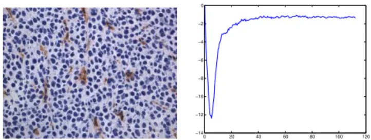
interpreted easily: L(r) = 0 means that the distribution of the process is completely random at scaler; positive maximal values account for a clustering behavior whereas negative minimal values point out regularity at the corresponding scale (Fig. 2). In addition, it is a cumulative measure whose estimation does not need any arbitrary kernel smoothing unlike the pair correlation function.
0 20 40 60 80 100 120 −14 −12 −10 −8 −6 −4 −2 0
Fig. 2. An ectopic model image at the 15th
day (left) and its corresponding L-function (right): The negative peak shows strong evidence of regularity at this scale.
To make sure that the spatial dependence is not related to a first order effect such as density, we assume that the obtained point patterns are stationary and isotropic. These assumptions are plausible for our image database (Fig. 1). Based on these assumptions and since we have a rectangular region of interest, the most appropriate edge correction method when computing L is the toroidal one [12].
2) Analysis of Variance for Functional Data: In order to find whether the obtained L-functions have significantly different values according to both the day after tumor implant and the animal cancer model (ectopic and orthotopic), we use an analysis of variance for functional data (fANOVA).
ANOVA is a statistical method that models a quantitative variable as a function of qualitative factors. Each factor can take several values, called levels, and ANOVA allows to compare the means of two or more groups defined by these levels by testing the null hypothesis H0: ”the different levels
have equal means”. In our study, the quantitative L-functions can be described along two factors: the day after tumor implant which has four levels (11, 15, 18 and 21) and the cancer model which has two levels (ectopic, orthotopic).
Two types of ANOVA will be considered in our results according to the number of factors taken into account:
• A two-way ANOVA tests the influence of both factors
simultaneously: that is the entangled impact of both the cancer model and the day after implant on L-functions variability.
• A one-way ANOVA considers each factor separately. It can be used to determine which precise levels are responsible for the null hypothesis failing if the two-way ANOVA test is rejected.
Since we are dealing with functional data (the L-functions), we choose to use the method proposed in [13]. Basically, this method uses random projections to transform functional data into univariate data and then solves the obtained simple scalar ANOVA problem. We obtain conclusions for the functional
data by collecting the information from sets of several pro-jections with p-value correction based on the False Discovery Rate (FDR). This method is flexible, easy to compute and requires no normality assumption.
IV. RESULTS ANDDISCUSSION
A. Objects’ Centroid Extraction
We compute the topographic map for each image in our database. Following the filtering criteria explained in Sec-tion III-A, we get the objects’ locaSec-tions. Figure 3 shows one result on a cropped area. Results over the whole database have been qualitatively evaluated and are visible online1. The
proposed extraction method has several important advantages: It is invariant to local contrast and it does not require fine threshold tuning or an object pre-detection step. We can thus apply the same procedure and parameter value (object physical size) to all images. The combination of dimension and topological criteria acts as a bidirectional filtering in the tree structure: the dimension threshold cuts the lower lines (noise) whereas the subsequent leaf threshold cuts the lines that could enclose more than one object. This trade-off is a typical problem in binarization methods which seek to obtain disjoint clusters of pixels [7]. Finally, the computation of the topographic map is fast, and the implementation of the whole method, including the manipulation of the level-lines as polylines is straightforward.
(a) Input image (b) Filtered map (c) Centroids
Fig. 3. Object extraction on a cropped example. Computing the topographic map of the input image (a), we apply successive filtering criteria providing a set of disjoint level-lines (b). The centroids of these filtered tree’s leaves represent the object locations (c).
B. L-Functions Estimation
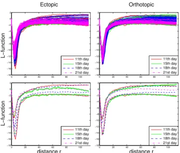
For each image, we estimate the L-function on the obtained point distribution along a vector of distances0 < r < 114µm. This upper bound corresponds to the common practice of choosing the one-half of the shortest image dimension [14]. The L-functions estimated over the whole database strongly overlap due to their high visual similarity (top row of Fig-ure 4). We thus also show the envelopes of the L-functions for each model and each day (bottom row of Figure 4). The negative peak around 5µm points out a strong regularity behavior at this scale. This is due to the typical interspace distance between cells. By only observing these functions and envelopes, we cannot conclude whether there are significant differences in the spatial organizations between the different days, or between the two models.
Fig. 4. (top) The 355 L-functions estimated over the whole database strongly overlap due to their high similar content. (bottom) The L-functions’ envelopes show their amplitude range for each day and model.
C. fANOVA Application
Intra Group fANOVA As a sanity check, we first test the null hypothesis within each single group (day/model). We randomly separate each of the groups into two parts, and we use one-way fANOVA between these two parts. We repeated this test 1000 times per group. The obtained p-values (p > 0.05) state that H0 is accepted for all groups
considered separately. This ensures that the potential inner group variabilities, such as the mice variability, do not affect subsequent results.
Two-Way fANOVA We use the functional ANOVA frame-work presented in Section III-B to test the existence of factors’ interaction. The obtained p-values indicate thatH0is rejected
and the interaction exist (p < 0.05). This means that there is a significant difference in the spatial organization of the biological objects in the images according to both factors simultaneously.
One-Way fANOVA We use the fANOVA with each factor separately to find where exactly the significant differences occur. We first test H0 for each day between the two models
(see diagonal of Table II). The results show that there are significant differences between the two models at days 15, 18, and 21 whereas there are no differences at day 11. This suggests that after that day, the two models are no more similar in terms of the spatial behavior of the objects.
We also test the null hypothesis for each model between every pair of days (upper and lower triangles of Table II). For the ectopic model there are differences in the spatial organization at all days, whereas for orthotopic model there are no differences between the days 11 and 15 (see Table II). In other words, this suggests that the orthotopic model does not significantly evolve between these two days in terms of the spatial behavior, whereas the ectopic one does.
TABLE II
TEST OFH0FOR THEL-FUNCTION BETWEEN ALL PAIRS OF DAY AFTER IMPLANT FOR ECTOPIC MODEL IN LIGHT GRAY,FOR ORTHOTOPIC MODEL
IN GRAY,AND BETWEEN BOTH MODELS IN WHITE. “A”AND“R”STAND FORacceptedANDrejectedRESPECTIVELY. THE STAR EXPONENT MEANS THAT THE SAMEANOVATEST ON FIRST-ORDERdensity of objectsGIVES
AN OPPOSITE ANSWER. Day 11th 15th 18th 21th 11th A A⋆ R⋆ R 15th R⋆ R⋆ R R 18th R⋆ R R⋆ R 21th R R R R⋆
D. Comparison With a First-Order Descriptor
We compare the proposed second-order descriptor with a first-order descriptor: the density of objects. The star exponents in Table II show where the scalar ANOVA test for the density value gives a different result. Along the diagonal for instance, the results indicate that this first-order descriptor detects no differences between the ectopic and the orthotopic model at all days. The null hypothesis is indeed always accepted. This observation stresses the added insights given by the second order analysis.
V. CONCLUSION ANDFUTUREWORK
We proposed a framework that automatically extracts the locations of the objects of interest in histology images. Based on a second-order function, that measures the spatial interac-tions on a continuous scale range, and a functional analysis of variance, we are able to assess the differences along both the cancer model and the day after implant. Note that the two considered cancer models visually produce highly similar images. However, the proposed second-order framework ac-counts for significant differences where the classic first-order density feature does not detect any. This advocates for the complementary use of first and second order features to better compare the models used by biologists.
We plan to address the following limitations in the near future. First, measuring the intra- and inter-correlation between the different types of the biological objects, such as cells’ nuclei and vessels populations, would give more specific insights to the entangling of the underlying behavior. In fact, vascularization plays a key role in tumor evolution. Secondly, our next goal is to propose statistical features that not only assess the differences between two groups of images with respect to the presented factors, but also measure these dif-ferences with a metric. This would eventually enable ordering the groups based on their relative distances.
ACKNOWLEDGMENTS
This work has been partially supported by the ANR SPIRIT #11-JCJC-008-01.
REFERENCES
[1] Heldmuth Latorre Ossa, In vivo monitoring of elastic changes during
cancer development and therapeutic treatment, Ph.D. thesis, Université Paris Diderot, 2012.
[2] G.M. Cooper, The Cell: A Molecular Approach, Sunderland (MA): Sinauer Associates, 2nd edition, 2000.
[3] J. Illian, P.A. Penttinen, H. Stoyan, and P.D. Stoyan, Statistical Analysis
and Modelling of Spatial Point Patterns, Statistics in Practice. John Wiley & Sons, 2008.
[4] J. E. Besag, “Comments on ripley’s paper,” Journal of the Royal Statistical Society, vol. B39, pp. 193–195, 1977.
[5] T. Mattfeldt, S. Eckel, F. Fleischer, and V. Schmidt, “Statistical analysis of labelling patterns of mammary carcinoma cell nuclei on histological sections.,” Journal of Microscopy, vol. 235, no. 1, pp. 106–118, 2009. [6] A Francesca Setiadi, Nelson C Ray, Holbrook E Kohrt, Adam Kapelner,
Valeria Carcamo-Cavazos, Edina B Levic, Sina Yadegarynia, Chris M van der Loos, Erich J Schwartz, Susan Holmes, and Peter Lee P, “Quantitative, architectural analysis of immune cell subsets in tumor-draining lymph nodes from breast cancer patients and healthy lymph nodes,” PloS one, vol. 5, no. 8, 2010.
[7] Y. Jiao, H. Berman, T.R. Kiehl, and S. Torquato, “Spatial organization and correlations of cell nuclei in brain tumors.,” PLoS One, vol. 6, no. 11, pp. e27323, 2011.
[8] L.A. Waller, A. Särkkä, V. Olsbo, M. Myllymäki, I.G. Panoutsopoulou, W.R. Kennedy, and G. Wendelschafer-Crabb, “Second-order spa-tial analysis of epidermal nerve fibers.,” Statistics in Medicine, p. 2827–2841, 2011.
[9] Y. Al-Kofahi, W. Lassoued, W. Lee, and B. Roysam, “Improved automatic detection and segmentation of cell nuclei in histopathology images,” IEEE Trans. on Biomedical Engineering, vol. 57, no. 4, pp. 841–852, 2010.
[10] V. Caselles and J. M. Morel, “Topographic maps and local contrast changes in natural images,” International Journal of Computer Vision, vol. 33, pp. 5–27, 1999.
[11] J. Serra, Image Analysis and Mathematical Morphology, Academic Press, 1982.
[12] I. Yamada and P. Rogerson, “An empirical comparison of edge effect correction methods applied to k-function analysis,” Geographical Analysis, vol. 35, no. 2, pp. 97–109, 2003.
[13] J.A. Cuesta-Albertos and M. Febrero-Bande, “A simple multiway anova for functional data,” TEST: An Official Journal of the Spanish Society of
Statistics and Operations Research, vol. 19, no. 3, pp. 537–557, 2010. [14] Philip M Dixon, “Ripley’s K function,” Encyclopedia of environmetrics,