HAL Id: halshs-01311487
https://halshs.archives-ouvertes.fr/halshs-01311487
Submitted on 4 May 2016
HAL is a multi-disciplinary open access archive for the deposit and dissemination of sci-entific research documents, whether they are pub-lished or not. The documents may come from teaching and research institutions in France or abroad, or from public or private research centers.
L’archive ouverte pluridisciplinaire HAL, est destinée au dépôt et à la diffusion de documents scientifiques de niveau recherche, publiés ou non, émanant des établissements d’enseignement et de recherche français ou étrangers, des laboratoires publics ou privés.
Interdependencies between Atlantic and Pacific
agreements: Evidence from agri-food sectors
Anne-Célia Disdier, Charlotte Emlinger, Jean Fouré
To cite this version:
Anne-Célia Disdier, Charlotte Emlinger, Jean Fouré. Interdependencies between Atlantic and Pacific agreements: Evidence from agri-food sectors. Economic Modelling, Elsevier, 2016, 55, pp.241-253. �10.1016/j.econmod.2016.02.011�. �halshs-01311487�
1
Interdependencies between Atlantic and Pacific Agreements:
Evidence from Agri-food Sectors
♦Anne-Célia Disdiera,∗ Charlotte Emlingerb Jean Fouréc
a PSE-INRA, 48 boulevard Jourdan, 75014 Paris, France
b Charlotte Emlinger, CEPII, 113 rue de Grenelle, 75007 Paris, France
c Jean Fouré, CEPII, 113 rue de Grenelle, 75007 Paris, France
Abstract
Trade liberalization of the agri-food sector is a sensitive topic in both Transatlantic Trade and Investment Partnership (TTIP) and Trans-Pacific Partnership (TPP) discussions. This article provides an overview of current trade flows and trade barriers. Then, using a general equilibrium model of international trade (the MIRAGE model), it assesses the potential impact of these two agreements on agri- food trade and production. The results suggest that the US agri-food sectors would gain from both agreements while almost all their partners and third countries would benefit less, and might register losses in some sectors. However, the two agreements are not competing, since all the contracting parties’ interests are complementary. Finally, we show that the Atlantic trade may be impacted by the inclusion of harmonized standards within the Pacific agreement but not by its extension to additional members (e.g. China or India).
Keywords: Mega-trade deals; agri-food; CGE model; Transatlantic Trade and Investment Partnership; Trans-Pacific Partnership
JEL: F13; F15; Q17
♦ This paper was initially circulated under the title “Atlantic versus Pacific Agreement in Agri-food Sectors: Does
the Winner Take it All?”. With the usual disclaimers, we would like to thank Sébastien Jean, Lionel Fontagné, Houssein Guimbard, Gianluca Orefice, and participants at GTAP 2015, AAEA 2015, ETSG 2015 and at the workshop on “Macroeconomics of Agriculture and Development” for their helpful advices. We are grateful to Sushanta Mallick and the two anonymous referees for their suggestions. A preliminary version of the paper was financed by the European Parliament’s Committee on Agriculture and Rural Development.
∗ Corresponding author at: 48 boulevard Jourdan, 75014 Paris, France.
2
1. Introduction
Preferential trade agreements have proliferated since the beginning of the 2000s. How- ever, until recently, their impact on trade and economic growth has been limited (Erixon, 2013). In 2008, only 16% of world trade benefited from preferential tariffs (WTO, 2011) but things are changing with the emergence of so-called mega-trade deals. Regional openness is becoming a major challenge for many countries, while multilateral liberalization, following the collapse of the Doha round negotiations, is being relegated to the sidelines. These mega-trade deals are seen as a way to compensate unsuccessful multilateral negotiations, to cope with issues not yet tackled by the World Trade Organization (WTO), and to benefit from the dynamic economic growth taking place in some areas (Francois, 2014). They are comprehensive agreements which by integrating markets, often go beyond tariffs. Given their size and ambitions, they are fundamentally different from the old regional trade agreements. They are likely to have systemic implications for the world economy and the future distribution of world trade flows (Cernat, 2013; Erixon, 2013) and are a source of fears for some citizens.
The Transatlantic Trade and Investment Partnership (TTIP) and Trans-Pacific Partnership (TPP) are perfect illustrations of these mega-trade deals. First, they involve countries that respectively represent 46% and 39% of world GDP. Second, they aim at removing trade barriers in a wide range of sectors to ease the exchange of goods and services between partners. The TTIP involves the United States (US) and the European Union (EU), and deals with the removal of the remaining tariffs, and the harmonization of non-tariff measures (NTMs). The TPP currently includes the US and 11 other countries and tariff liberalization is the main part of the agreement.
Policy makers have huge expectations of both agreements. On November 14, 2009, President Obama committed the US to engaging “with the TPP countries with the goal of shaping a regional agreement that will have broad-based membership and the high standards worthy of a 21st century trade agreement” (Fergusson et al., 2015). Shortly after the launch of the TTIP negotiations on February 13, 2013, European Commission President Barroso declared “A future deal will give a strong boost to our economies on both sides of the Atlantic” (Barroso, 2013).
The potential for competition between these two mega-deals and their effects on third countries are open questions. For the TTIP and TPP countries, the cost of a non- agreement is not simply the status quo in terms of trade but potentially could result in isolation from dynamic markets, especially in the context of a successful concurrent agreement. Similarly, both agreements may indirectly affect third countries. Although it had no official status in the TPP negotiations, China showed a growing interest in the negotiations. Anticipating the potential consequences of a TPP deal for its economy, the Chinese authorities have begun to focus more closely on the discussions and their conclusions, and may join the agreement in the future.
While these agreements involve the whole economy, in some sectors the negotiations are rather sensitive. Despite the relatively small share of agriculture in global output and employment, it is a definite hot topic. The issues being raised relate to anxieties over food security, food safety, and poorer health and environmental standards, but the spatial concentration of agricultural production also makes the question of agricultural wages very sensitive. Furthermore, cultural differences can complicate the TTIP negotiations in agri-food
3
sectors. In relation to risk management, Europeans advocate the precautionary principle, and worry about the ‘risk proven approach’ generally favoured by the US. At the same time, due to the current level of protection, agri-food flows across TTIP and TPP countries are relatively weak compared to exchanges of manufactured goods, and significant trade potentials exist.
This paper provides a simulation of the trade and production impacts that might be
expected from these mega-trade deals. We focus on the agri-food sectors1 and use a computable
general equilibrium model (CGE). CGE models have shown to be an accurate approach to assess Free Trade Agreements outcomes (Hertel et al., 2007). This approach allows us to highlight the sector effects of trade deals and the global interactions between markets. We rely on the CGE model MIRAGE.
Our contributions to the existing literature on quantification of the effects of mega-deals, and more precisely on the TTIP and TPP, are fourfold. First, our paper provides a detailed assessment of the impact of these two agreements on agri-food trade. Based on the current set of participating countries, these agreements cover 12% of world agri-food trade flows in 2012 (excluding intra-EU trade). The impact is further decomposed by country and sector. Recent papers have separately examined the impact of the TTIP (Erixon and Bauer, 2010; Fontagné et al., 2013; Francois et al., 2013; Felbermayr et al., 2013; Bureau et al., 2014; Beckman et al., 2015; Felbermayr et al., 2015; Egger et al., 2015) and TPP (Burfisher et al., 2014; Petri et al., 2011) using CGE analysis. However, we are the first to explicitly compare these two regional
trade agreements.2 Furthermore, our inclusion of agri-food trade goes comparatively deeper.
Second, CGE simulations require the use of accurate measures of trade policies. The agri-food sector continues to be affected significantly by public interventions. For tariff barriers, we rely on the MAcMap database which offers a disaggregated (at the 6-digit level of the Harmonized System - HS), exhaustive, and bilateral measure of the protection applied by importing countries on each product. It includes tariff preferences, tariff rate quotas, and ad valorem equivalents (AVEs) for all non-ad valorem duties. In addition, we estimate AVEs of NTMs. In CGE simulations, harmonization of NTMs translates into a cut in their trade restrictiveness, i.e. in their AVEs. AVEs of NTMs are computed at the product level using countries’ notifications to the WTO of sanitary and phytosanitary measures (SPS) and technical barriers to trade (TBT). Our coverage is exhaustive, since we include all countries notifying their NTMs to the WTO. We rely on the method suggested by Kee et al. (2009), which consists of estimating the trade effects of these NTMs and converting them into AVEs using import demand elasticities.
Third, we contribute to the literature on CGE evaluation of trade deals by introducing more differentiation among countries in terms of NTM effects through aggregation (on a single market, all partners do not face the same trade-restrictiveness), and departing from the usual assumption that the cost effect of a NTM is a pure efficiency loss. Indeed, NTM efficiency costs are less evident than welfare losses associated with tariffs and quantity barriers. By omitting these effects, the usual NTM impact computed in the trade literature is significantly biased. Furthermore, we model the economy – and especially the agri-food sector – with as much detail
1 Agri-food sectors include products covered by the WTO Agreement on Agriculture plus fish and fish products. 2 Jurenas (2015) investigates the potential effects of TPP and TTIP. However, the study does not provide new
4
as possible. We consider 31 distinct sectors, of which 16 are related to agri-food products. Our approach therefore provides insights on how CGE models can be used to investigate the trade and production effects of multiple trade agreements signed simultaneously on both member and third countries.
Fourth, we test the sensitivity of our results by considering different trade liberalization schemes. More precisely, we assume various levels of tariff and NTM cuts. We also simulate alternative boundaries for the TPP Agreement: deep integration with harmonization of NTMs alongside tariff cuts, and broad geographic coverage with additional members such as China, India, and South Korea among others.
Our results suggest first that both agreements might have comparable effects in terms of their magnitude on world food trade flows. The US would be the main winner in the agri-food sectors, though an Atlantic deal would be more profitable overall to the US than the Pacific agreement. The US applies lower tariffs than its potential FTA partners on its imports and its production is specialized in sectors facing high NTMs in destination markets. Our results suggest also that the impact of both agreements could be (almost) additive for the US and not competing due to a relatively elastic supply of agri-food products despite the similarity among US offensive interests in the Pacific and Atlantic markets.
In terms of trade diversion, the Pacific countries have more to lose from the conclusion of the TTIP Agreement than does the EU from the achievement of the TPP agreement. This is due mainly to their relative specialization which does not match perfectly with the US market. Finally, the magnitude of the effects could be significantly affected by the form of the TPP Agreement. While a deeper agreement (including NTM cuts) could significantly reduce EU agri-food exports to the US (price competition is affected more by NTMs than by tariffs), a broader TPP including China and India among other countries would affect EU agri-food exports very little and might even trigger trade increases in some sectors. This last result can be explained by the complementarity in terms of specialization between potential TPP members and the EU.
Our paper is organized as follows. Section 2 provides an overview of TTIP and TPP negotiations, trade patterns, applied tariffs and NTMs. Section 3 presents the CGE modelling framework and describes the simulation scenarios. Section 4 reports the impacts of the two agreements separately and checks the sensitivity of our results to the simultaneity and characteristics (boundaries and trade liberalization) of the two agreements. The paper concludes in the Section 5.
2. Atlantic and Pacific trade patterns
This section presents the main characteristics of the TTIP and TPP areas in terms of trade flows and trade barriers.
2.1. Which framework for which negotiations?
The main feature of the TTIP and TPP deals is their huge size (Table 1). In 2012, TPP members accounted for 11.3% of the world population, 38.5% of world gross domestic product (GDP), and 27% of world trade (import and export). The TTIP area accounted for 11.6% of the world population, 45.8% of world GDP, and 25% of world trade. Finally, these two agreements cover 12% of world agri-food trade flows in 2012 (excluding intra-EU trade and using the current set
5 of participating countries).
Discussions regarding transpacific trade liberalization started in 2003 and involved Chile, New Zealand, and Singapore. The list of participants expanded over time to include Brunei (2005), the US, Australia, Peru and Vietnam (2008), Malaysia (2010), Canada and Mexico (2012) and finally Japan (2013). Negotiations dealt mainly with the dismantling of tariff barriers. In November 2011, TPP countries announced their objective to remove all tariff barriers on trade in goods with the coming into force of the TPP Agreement (with adjustment periods for sensitive products). Some tariffs were already abolished since each negotiating countries was involved in a free trade agreement (FTA) with at least one other TPP partner. An agreement was successfully concluded in October 2015. The text of the agreement is not currently publicly available. However, one can assume that trade liberalization mainly concern tariffs, while NTMs are less likely to be removed. Discussions on NTMs surround ensuring that as tariffs are reduced, they are not replaced by other forms of protection such as NTMs. TPP country coverage may be extended in the future. Several countries including Bangladesh, Cambodia, Colombia, India, Indonesia, Laos, Philippines, South Korea, and Thailand, have expressed interest in joining the group. The potential benefits of TPP membership (or the cost of remaining outside the TPP Agreement) are also being recognized increasingly by the Chinese authorities with the result that China is likely to take part in the future agreement.
At first glance, the transatlantic discussions involving just the US and the EU seem more straightforward. The European Commission has a mandate from the EU members to negotiate the TTIP. Negotiations began in 2013 and include the removal of remaining tariffs and the harmonization and/or mutual recognition of regulations and technical requirements. Multiple different rules are costly, and regulatory convergence is one way to reduce these costs. However, this is not always easy, and discussions over specific issues such as geographical indications, genetically modified organisms (GMOs), etc. have proved to be complex.
Table 1: TTIP and TPP characteristics
TTIP TPP
Members
Current EU28, US Australia, Brunei, Canada, Chile,
Japan, Mexico, New Zealand, Malaysia, Peru, Singapore, US, Vietnam
Potential Bangladesh, Cambodia, Colombia,
India, Indonesia, Laos, Malaysia, South Korea, Thailand (and China)
Negotiations
Start 2013 2011 (concluded in October 2015)
Focus Tariffs and NTMs Tariffs (and NTMs)
Key statistics (%, 2012)
Share in world population 11.6 11.3
Share in world GDP 45.8 38.5
Share in world trade 25 27
Note: Key statistics for TPP are computed on the sample of current members. Intra-EU trade is not included. Sources: World Development Indicators for population and GDP; CEPII-BACI database for trade flows.
6
2.2. Trade patterns3
Transatlantic trade relationships are already well developed. In 2012, flows between the EU and the US represented 4% of world trade. The EU market is the second main destination (after Canada) for US exports, and receives 16% of total US exports (USD 238 billion). At the same time, the US is the main trading partner of EU exporters (14% of EU total exports, i.e. USD 353 billion). In terms of imports, the EU is the second most important origin of US imports (16% of total imports), while the US is the third main origin of EU imports (10% of total imports) after China and Russia. Agri-food represents 10% and 8% respectively of US and EU overall exports. In terms of bilateral trade, 9% of US agri-food exports go to the EU and 11% of EU agri-food exports go to the US. Agri-food trade is concentrated in few sectors: 57% of European exports comprise the beverages and tobacco sector (mainly wine), while beverages and tobacco products, oil seeds, and fruit and vegetables account for half of US exports to the European market (see Figure A.1 in the Appendix for a detailed decomposition of agri-food trade by sector).
The TPP area is comparatively very heterogeneous. TPP flows are characterized by the prominence of NAFTA, and the role of Japan. Intra-NAFTA flows represent 59% of trade between TPP members (55% for agri-food). Canada and Mexico account for 40% of US total exports and 27% of its agri-food exports. The US is also the main export partner for Canada and Mexico, accounting respectively for 73% and 71% of their total exports (68% in agri-food). Japan plays the role of a link between the American and Asian sides of the TPP area. Japan is the second main exporter in the TPP region after the US. Its main export partner is the US (18% of Japanese exports go to the US; by comparison, only 5% of US exports go to Japan). Japan is also an important trading partner for several Asian countries (e.g. Brunei, Malaysia and Vietnam), Chile, and New Zealand. TPP countries vary also in the size of their agri-food trade. New Zealand has a strong specialization in agri-food (60% of its total exports), and this sector constitutes more than 15% of Australian and Chilean exports, and around 10% of US and Peruvian exports. By contrast, the share of agri-food products in exports from Japan and Brunei is very small (less than 1%). Meat, fruits and vegetables and cereals are the main products traded between TPP members (Figure A.1. in the Appendix.).
2.3. Tariff barriers
Although the tariff barriers affecting transatlantic and transpacific trade have been significantly reduced over the last few decades some are still in place, especially in agri-food sectors. Table 2
provides some figures extracted from the MAcMap-HS6 database4 jointly developed by the
CEPII and the International Trade Centre (ITC). These data are based on bilateral customs tariffs and include tariff preferences, tariff rate quotas, and AVEs for non-ad valorem duties which apply to 6% of agri-food tariff lines (compared to 0.6% of industry tariffs). AVEs are aggregated using the reference group method. This alternative weighting scheme reduces the
3 All statistics are computed excluding intra-EU trade flows. These statistics are based on the BACI database. This
database is developed by the CEPII and uses original procedures to harmonize United Nations COMTRADE data (evaluation of the quality of country declarations to average mirror flows, evaluation of cost, insurance and freight rates to reconcile import and export declarations, http://www.cepii.fr/cepii/fr/bdd_modele/presentation.asp?id=1).
7
endogeneity problem compared to the classic trade weighted scheme (for more details, see below and Guimbard et al., 2012).
EU-US bilateral applied protection follows four patterns. First, agri-food imports are more protected than non agri-food imports in both the US and the EU. Second, average EU protection related to US agri-food products is twice as high as the corresponding US protection (12.9% vs. 6.4%). Third, the EU imposes higher duties on a large share of agri-food products: 28.7% of such products (defined at the HS 6-digit level) imported by the EU from the US attract a high tariff (AVE above 15%). The corresponding rate is 6.5% for US agri-food imports from
the EU. Fourth, at the sector level,5 four groups of US agri-food products have high EU tariffs:
red meat (average of protection of 75%), dairy (38%), white meat (31%), and sugar (24%), which contrasts with tariffs of less than 5% for oil seeds, plant fibres, oils and fats. The highest levels of protection apply to European sugar at the US border (24%), followed by dairy products (19%). Other EU agri-food sectors are much less affected by US tariffs, with protection at levels below 7%.
Within the TPP area, TPP countries (excluding the US) protect more their imports than the US (higher average tariffs and higher share of tariff peaks). Besides, agri-food products attract higher tariffs on average than industry goods. However, the level of bilateral protection applied varies widely across countries, and is driven mainly by the existence of FTAs between some country-pairs (Table A.1 in the Appendix). For example, since the NAFTA, US agri-food tariffs on Mexico and Canada have been very low on average. Tariffs are also low at the US border for agri-food products from Chile, Peru, and Singapore since the US has in place FTAs with these countries. Similarly, Canadian agri-food protection is very low on average for FTA-partners (Mexico, Peru) but quite high for other importers (Japan, New Zealand, Singapore). There is a similar disparity in Mexican tariffs. Among the other TPP members, Australia applies very low agri-food duties on all imports (maximum 2%), while Japan generally imposes high tariffs. At sector level, dairy products are affected by high tariffs in several TPP countries (for example over 100% in Canada). Cereals are generally well protected (over 200% in Japan, mainly due to the very high levels imposed on rice). Finally, Mexican imports of sugar from other TPP countries (except the US) are subject to a tariff of 97% on average.
8
Table 2: Average applied protection on transatlantic and transpacific trade, 2010 (%)
Agri-food Non agri-food
Applied protection (%) Share peaks (%) Applied protection (%) Share peaks (%) Transatlantic trade
US tariffs applied to EU imports 6.4 6.5 1.7 1.9
EU tariffs applied to US imports 12.9 28.7 2.3 0.9
Transpacific trade
US tariffs applied to TPP imports 2.7 4.8 0.7 0.9
TPP tariffs applied to US imports 7.7 9.0 1.6 7.3
TPP tariffs applied to TPP imports (excl. US) 12.5 10.6 2.1 7.8
Note: Authors’ computation using MAcMap-HS6 database. Tariff peak: AVE above 15%.
2.4. Non-tariff measures
The reduction in tariffs under successive GATT/WTO agreements, and growing concerns among consumers about food safety and quality, has resulted in an increasing role of NTMs in international trade. Agri-food products are heavily affected by NTMs (UNCTAD, 2005). Unlike the case of tariffs, the trade and welfare effects of NTMs are ambiguous. Firstly, regulations are often necessary to prevent market failure, and to correct negative externalities; however, domestic regulations can be imposed simply to deter imports from foreign competitors (Beghin, 2008). Secondly, the implementation process required to comply with NTMs is costly, and may exclude some producers from the market. However, NTMs can contribute to improving market access by enhancing the reputation of foreign products. In such cases, NTMs can act as catalysts for trade.
2.4.1. Sources and descriptive statistics
Our analysis focuses on the two main types on NTMs adopted by TTIP and TPP countries that affect trade flows, namely the sanitary and phytosanitary measures (SPS) and technical barriers to trade (TBT) measures. These measures are classical “behind the border” costs and impact trade (Khan and Kalirajan, 2011). We use the notifications made by these countries to the
WTO.6 Each notification provides information on the notifying country (the importer), the
6 These notifications are used by the WTO in its 2012 World Trade Report (WTO, 2012) and are available via the
Integrated Trade Intelligence Portal (I-TIP) (https://www.wto.org/english/res_e/statis_e/itip_e.htm). Product codes are often missing from the I-TIP database and were added at the 4-digit level of the Harmonized System by the Centre for WTO Studies of the Indian Institute of Foreign Trade (http://wtocentre.iift.ac.in/). The recent NTM data collected jointly by the World Bank, the United Nations Conference on Trade and Development, and the African Development Bank and available on the WITS (World Bank’s portal for trade data) were not suitable for the present research since country coverage is limited (data are missing for 8 of the 12 TPP countries, including the US).
9
affected product (at the HS 4-digit level), and the type of measure (SPS vs. TBT). We include all measures notified up to the end of 2012. Our dataset is therefore more up to date than that developed by Kee et al. (2009) which was the basis for several previous studies.7 However, WTO members are required to notify only new or changed measures, and the notification requirements apply only to measures which differ from international standards, guidelines, or recommendations, or to situations where no standards exist, and, in addition may have a significant impact on trade. As pointed out in the literature, this could affect the results of an analysis of their trade (and welfare) impacts.
In almost all cases, NTMs are unilateral measures, i.e. they apply to a given product regardless of its origin. Furthermore, the principle of mutual recognition applies among EU Member States. According to this principle, goods and services can move freely across Member States, and national legislation does not have to be harmonized. Therefore, to avoid bias, we exclude intra-EU trade flows from our NTMs analysis.
A very large share of products is affected by NTMs in the US, the EU and TPP countries. These countries notify NTMs on almost all agri-food products. For non agri- food ones, the notification rate is slightly smaller but still very high: 78.6% of HS6 non agri-food products are affected by at least one NTM (SPS and/or TBT) in the US and more than 95% in the EU and TPP countries (without the US) taken as a whole. All sectors are affected by NTMs, with coverage ratios (i.e. the share of HS6 lines affected by at least one SPS or TBT within a sector) well above 50%. For the US, EU, and TPP countries, the coverage ratio is above 95% for all agri-food sectors.
2.4.2. Computation of AVEs of NTMs
To analyze the impact on trade of the NTMs notified by TTIP and TPP countries, we estimate AVEs, i.e. the level of ad-valorem tariffs that would have an equally trade- restricting effect as the focal NTMs. These AVEs are further used in the CGE simulations.
To compute the AVEs, we apply the method suggested by Kee et al. (2009). First, we estimate the quantity impacts of NTMs on trade flows, and then convert these effects into AVEs using import demand elasticities computed by Kee et al. (2008). We use the information on NTMs at the HS6 product level, and perform the estimations sector by sector. We define 25 sectors (16 of them are agri-food sectors) which are used also in the CGE simulations. Since the CGE model covers the whole world economy, our sample is extended to include non agri-food activities. Furthermore, third countries are included in addition to TTIP and TPP countries. We select all countries notifying NTMs to the WTO, and collect all measures adopted up to 2012. Our final sample includes 125 countries, and covers 92.5% of world trade flows in 2012. Lastly because of the strong correlation between SPS and TBT, we estimate the global effect of NTMs rather than the respective effects of SPS and TBTs.
Our dependent variable, Mrsi, is the dollar value of imports of good i by country s from
country r. We consider only trade flows that are strictly positive in 2012.8 The estimated
7 Kee et al. (2009)’s NTM data are for year 2004 in the best case (and are likely to be older for some countries). 8 The absence of bilateral trade between some countries and for some products may be determined by other aspects
10 section trade equation is:
ln Mrsi = a0 + a1 tariffrsi + a2 NTMsi + a3 distrs + a4 cbordrs + a5 clangrs + FEr + FEs + FEi + εrsi (1)
where tariffrsi measures the bilateral applied protection on product i, while NTMsi is a dummy set to 1 if the importing country notifies at least one NTM on the product i (0 otherwise). Our tariff data come from the MAcMap-HS6 database and are for year 2010 (2012 tariffs are not available). NTMs are extracted from the WTO I-TIP database, and our trade data come from the BACI database. Both sets of data are for 2012. distrs is the bilateral distance
between both countries r and s and proxies for trade costs; cbordrs and clangrs are dummies to
control for common border and common language. These two last variables and distance are extracted from the CEPII database.9 FE
r, FEs and FEi are respectively exporter, importer, and
product fixed effects. εrsi is the error term. The country fixed effects incorporate size effects, and
also the prices and number of the exporting country’s varieties, the size of demand, and the importing country’s price index. They allow us to avoid the most common mis-specifications in the literature relying on the traditional simplest gravity framework, i.e. lack of control for unobserved relative prices (Baldwin and Taglioni, 2006).
Estimations are run sector-by-sector. The estimated coefficients for the trade restrictiveness of NTMs, a2, in equation (1) are specific to each HS-4 level category, and are
constant worldwide. We convert them into importer-HS6 specific AVEs, denoted αs,i using the
import demand elasticities εs,i provided in Kee et al. (2008):10
i s, 2 i s, 1 -) exp(
ε
α
= a (2)Table 3 reports some of the summary statistics for these importer-HS6 AVEs for the TTIP and TPP countries. First, the mean AVEs are quite high, especially compared to tariffs (Table 2). Second, mean AVEs are slightly higher in the EU than in the US and the TPP countries (excl. US): 15.0% on all products for the EU versus 12.8% for the US and 10.0% for the TPP countries. Third, the breakdown into agri-food and non agri-food products show much higher AVEs of NTMs for agriculture. This (expected) result holds for all countries. The mean AVEs for agri-food products in the US and EU are about four times bigger than the mean AVEs for non agri-food products, and about 7 times bigger in the TPP countries (excl. the US).
attribute these zeros to restrictive tariffs and/or NTMs.
9http://www.cepii.fr/CEPII/en/bdd_modele/presentation.asp?id=6.
10 These elasticities are computed for the beginning of the 2000s, and remain the only ones currently available in the
11
Table 3: Estimation of AVEs of NTMs: summary statistics, 2012 (%) Mean
All Agri-food Non
agri-products agri-products products
US 12.8 35.7 8.7 (38.7) (66.7) (29.2) EU 15.0 40.1 10.4 (24.8) (45.8) (14.6) TPP countries 10.0 36.7 5.1 (23.6) (47.1) (10.1)
Note: Authors’ computation. Mean AVE: simple average across HS6 products. TPP countries: simple average across countries (US excluded). Standard deviation across products in parentheses.
Although seemingly large in magnitude, our AVEs for agri-food products are around 10 points lower than those computed by Kee et al. (2009). These differences may be due to the time period covered by the data (2004 for Kee et al. (2009) and 2012 for our data), and the country and product coverage. Our data include some products and several EU and TPP countries that are missing from Kee et al. (2009)’s sample.
3. Modelling framework
Evaluating the potential impact of trade agreements on the world economy leads to many issues from tariffs to NTMs which are combined with the medium-term trade pattern dynamics. Since a detailed and accurate analysis of all these issues for each sector is impossible, we propose a consistent framework to be applied to all sectors, in order to derive comparative conclusions about the substitutability or complementarity between the Atlantic and Pacific agreements. We
rely on MIRAGE (Modeling International Relationships in Applied General Equilibrium),11
which is a multi-sector and multi-regional computable general equilibrium model dedicated to trade policy analysis (Fontagné et al., 2013; Decreux and Valin, 2007; Bchir et al., 2002). Each sector is modelled as a representative firm with constant returns to scale (perfect competition). International trade follows an Armington specification (goods from different origins are not perfect substitutes) and is impacted by tariffs and NTMs. Consumers and the government are represented by a single agent by region, which maximizes its instantaneous utility function and owns all primary factors (skilled and unskilled labour, land, capital and natural resources). These factors are fully employed and are accumulated following the long-term projections provided by
the EconMap database (Fouré et al., 2013).12
CGE models have been used frequently to conduct ex-ante assessments of trade
11 A two-page summary of the model and the full set of equations is available in the online appendix
(http://annecelia.disdier.free.fr/MIRAGE_Equations_Appendix.pdf).
12
agreements. The framework they offer is relevant for a consistent investigation of the interdependencies between economies based on trade, and the feedbacks from income effects and factor markets.
3.1. Which impacts apply to which NTMs?
The main advantage of the CGE approach is its consistency and exhaustiveness, all world sectors and countries are included in the analysis. However, it is necessary to rely on a systematic methodology which requires some assumptions. To deal with NTMs, we rely on their AVEs. The very objective of such measures (health and/or environmental protection, etc.) cannot be incorporated in the model. Furthermore, some prohibitive measures cannot be explicitly modelled, especially if they are related to only one part of the sector’s output. For instance, we cannot distinguish hormone-fed and hormone-free beef. Nevertheless, we provide a different evaluation which contributes to the modelling literature in two ways. First, we refine the structure of potential costs implied by NTMs by exploiting the information available at the HS-6 digit level, in order to build precise and consistent bilateral AVEs (see above for their computation). Second, we allow for potential externalities related to rent creation due to the presence or imposition of NTMs (and rent reduction due to their harmonization) by introducing three different types of NTM modelling.
Several authors, for instance Walkenhorst and Yasui (2005) or Fugazza and Maur (2008), point to three different types of trade effects related to NTMs. The first is a direct increase in export costs due to the need to comply with specific requirements and/or to obtain certifications required to access the destination country’s market. This is called the “trade-cost” effect. The second corresponds to a “supply-shifting” effect: certain regulations or bans can reduce supply in some sectors (e.g. GMOs, hormone-fed beef). The third effect is a “demand-shifting” effect which occurs when NTM requirements (such as product labelling) affect consumer behaviour. The first two effects are trade-impeding, while the demand-shifting effect is ambiguous.
Fugazza and Maur (2008) point to the lack of empirical quantification of a supply- shifting and a demand-shifting effect. The authors acknowledge the possibility that NTMs may change the elasticity of substitution between imported goods, as well as between domestic and foreign goods in the Armington-style demand system. However, they are unable to find estimates of these potential changes. We are faced with the same data constraints, and are unable to integrate in our model the supply-shifting and demand- shifting effects.
However, our CGE simulations allow us to address the issue related to the “trade-cost” component of NTMs based on our estimations of NTM AVEs. Existing evaluations of trade agreements including NTMs, and of the TTIP and TPP Agreements in particular (Francois et al., 2013; Petri et al., 2011), consider this trade-cost effect as a pure efficiency loss (also called “sand-in-the-wheels”). However, this approach does not cover all the potential cost effects we can expect from implementation of a NTM. In particular, many measures are not neutral regarding income: they can imply a rent that is captured by one or other sides of the border. Furthermore, in the presence of licensing measures, monopolistic rents can benefit local governments or local/foreign firms (depending on the licence allocation method). These three different ways of considering a cost effect (no rent, rent attributed to locals, rent attributed to
13
foreigners) in our context of perfect competition and a single agent representing consumers and government are equivalent to the implementation of an efficiency loss, an import tax equivalent,
or an export tax equivalent (Walkenhorst and Yasui, 2005).13
The distinction between these cost effects and their equivalent is of prime importance. Their potential impacts on consumers’ real income are different, especially in relation to terms of trade (Andriamananjara et al., 2003). On the one hand, the political economy literature, following the seminal work by Grossman and Helpman (1994), advocates in favour of an allocation of rents generated by trade policies to domestic producers. Their framework states that the presence of tariff protection can be explained by the contributions of local lobbies. This theoretical framework has been tested – and validated – empirically in the presence of NTMs by Gawande and Bandyopadhyay (2000). On the other hand, there is no clear evidence on the part of NTMs settled to protect local producers instead of local consumers. Hence, it prevents us from drawing assumptions about the allocation of rents related to NTMs. Therefore, compared to the existing literature on CGE analysis, our approach regarding these cost effects remains agnostic – although as arbitrary; it splits the trade-restrictiveness effect of NTMs into three, allocated as one third to an efficiency loss, one third to generate rent for domestic producers, and one third to rent for foreign producers. This issue is further discussed in Section 3.3.2.
3.2. Data and aggregation
The CGE MIRAGE model is a flexible tool that can be tailored to respond to different policy questions. In the present case, we model the agri-food sector in as much detail as possible. We consider 31 different sectors (of which 16 are related to agri-food products), and 24 geographical areas. Detailed aggregations of sectors are provided in Table 4 and of regions in Table 5.
13 In our version of the CGE MIRAGE model, this corresponds to an iceberg cost, an additional import duty and an
14
Table 4: Sector aggregation
Agri-food Industry
Cereals Clothing
Vegetable, fruits and nuts Chemical, rubber and plastic products
Oil seeds Metal products
Sugar, sugar cane and beet Transport equipment
Plant-based fibres Electronic devices
Other crops Machinery and Equipment
Live animals Other manufacturing
Red meat Services
White meat Business Services
Milk and dairy products Transport
Other animal products Finance and insurance
Forestry Recreation and other services
Fishing Public administration
Vegetable oils and fats Other services
Beverages and tobacco products Energy and other primary
Other food products Energy
Other primary
Table 5: Country aggregation
European Union (28) Other countries
US Brazil
Other NAFTA Argentina
Canada European Free Trade Area
Mexico Other Europe
TPP Members Russian Federation
Australia and New Zealand Turkey
Chile and Peru Other Middle East
Singapore, Malaysia and Vietnam North Africab
Japan Other Africa
Other ASEANa Rest of the Worldc
TPP Potential members
China India Korea Other Asia
Other Latin America
Note: a: Cambodia, Indonesia, Lao PDR, Philippines, Thailand, Rest of Southeast Asia; b: Egypt, Morocco, Tunisia, Rest of North Africa;
c: Rest of Oceania, Rest of North America, Rest of the World.
MIRAGE relies on the Global Trade Analysis Project (GTAP) database for social accounting matrices (version 8.1). Tariffs are taken from the MAcMap-HS6 database (Guimbard et al., 2012) for years 2007 and 2010, and AVEs for NTMs in goods are our own estimations (see above). AVEs for NTMs in the service sector are taken from Fontagné et al. (2011).
15
and αs,i) the CGE MIRAGE model is not defined at this level of detail since it would require very complex data. Instead, the model only includes 24 regions and 31 sectors. When aggregating tariffs and AVEs at the country-HS6 level (r, s, i) to the MIRAGE aggregation level (R, S, I), we take advantage of two valuable pieces of information. First regarding NTMs, we consider the contribution of an HS6 line to the aggregate AVE only if at least one NTM is
actually implemented in the (r, s, i) trade flow, using the dummy variables δr,s,i constructed from
the WTO notifications. Second, the MAcMap-HS6 database provides information on the
weights ωr,s,i of each disaggregated flow which can be used to further aggregate the tariffs and
NTMs from the HS6 to the MIRAGE level. These weights are computed using the reference group method which requires each country to be allocated to one of five world regions (the reference groups) with similar characteristics, using hierarchical clustering analysis. The weight of each flow is the share of good i in the imports of the whole reference group originating from region r, scaled by the size of the imports of country s in its reference group (for more details, see Guimbard et al., 2012). The advantage gained by deriving these weights compared to simply weighting by trade flows is that they take account of at least part of the prohibitiveness of certain transaction costs. Letting G(s) denote the reference group of country s, and (ρ, ι) denote the country-HS6 level:
∑
∑
∑
−
=
ι s,G(s)ι ρ,ι ρ,G(s)ι ρ,ι ρ,s, ι r,G(s),i r,s,iM
M
M
M
, ,ω
(3)∑
∑
∈ ∈=
) , , ( ) , , ( , , ) , , ( ) , , ( , , , , , , , I S R i s r r s i I S R i s r r s i r s i s i I S Rave
ω
α
δ
ω
(4)∑
∑
∈ ∈=
) , , ( ) , , ( , , ) , , ( ) , , ( , , , , , , I S R i s r r s i I S R i s r r s i r s i I S Rtariff
ω
τ
ω
(5) 3.3. Scenario assumptionsThree main scenarios are defined in our analysis.
3.3.1. Business-as-usual
Before considering the counterfactual scenarios, a business-as-usual (BAU) pattern for the world economy which is the “baseline”, is simulated up to 2025. In order to have consistent projections for overall total factor productivity, and trajectories for production factors (labour force, education level, capital accumulation), we rely on macro-economic projections from the
EconMap database.14 Furthermore, we take account of three foreseeable changes to reflect the
14 For a detailed description of the MaGE model, which is used to produce the EconMap database, see Fouré et al.
16 context of potential Atlantic and Pacific agreements:
- Data update: MIRAGE base data is for year 2007 only but MAcMap tariff data are
available also for year 2010. We therefore implement a linear global tariff update between 2007 and 2010.
- The EU: We implement completion of the EU28 Single Market on the tariff side (full
liberalization of trade flows with the inclusion of Romania and Bulgaria in 2008, Croatia in 2013, and adoption of the EU external tariff by Croatia in 2013).
- Known free trade agreements: According to the WTO regional trade agreements
database,15 since 2007 numerous bilateral agreements have come into force, or been
signed and are due to take effect in subsequent years. We counted 100 in-force agreements, 5 signed agreements, and 23 agreements (apart from the TTIP and TPP) currently under negotiation. Our baseline scenario considers the first two categories (“in-force” and “signed”), and implements a simplified version of these agreements. Tariffs are reduced by 100% linearly but at different rates depending on the HS-6 line considered: (i) for half of the products (e.g. less sensitive products, i.e. HS-6 lines with the lowest initial tariffs) tariffs are set to zero the year the agreement comes into force; (ii) for 25% of the remaining products (e.g. less sensitive remaining ones) a linear liberalization in three years time; and (iii) for the remaining 25% of products (e.g. the most sensitive products, i.e. those with the highest initial tariffs) linear liberalization in
five years time. Thus, full liberalization takes place between 2008 and 2013.16 While this
might seem a rather unrealistic assumption, our objective is to prevent our results from attributing to the TTIP and TPP Agreements the outcomes of already-signed agreements. The economic impacts of the Atlantic and Pacific agreements are computed as the difference between a path incorporating their enforcement, and this baseline.
3.3.2. Scenarios for the Atlantic and Pacific agreements
In the case of both agreements, we implement full tariff liberalization using the same scheme as in the BAU scenario: HS-6 lines are split depending on their initial tariffs, with differentiated reduction speeds: instant liberalization for half of the lines (the less protected ones), liberalization in three years for half of the remaining lines, and liberalization after five years for
the 25% most sensitive lines.17
The Atlantic liberalization: On the tariff side, we implement full liberalization between 2015
and 2020. The potential outcome in terms of NTMs is less easy to predict. The literature relies on a single evaluation proposed by Ecorys (2009) – 25% reduction in the trade-restrictiveness of
15 RTA-IS available at http://rtais.wto.org/UI/PublicMaintainRTAHome.aspx, accessed June 2014. 16 In the remainder of this paper, the term “full liberalization” refers to the same scheme.
17 In MAcMap-HS6, the applied tariff AVE for a product under a Tariff Rate Quota (TRQ) is the relevant marginal
rate of the TRQ (depending on the quota fill rate). In our scenarios, AVEs for products with TRQs are set to zero, following the scheme for other products. This assumption may have a non- negligible impact on the European beef sector where TRQs are important.
17
NTMs which is not a measure of the potential outcome of negotiations but rather half the reduction that European and American entrepreneurs and regulators think is achievable assuming the political will for its achievement. Although this is not completely satisfactory, it is the only information available. Therefore, we assume a 25% cut in the trade restrictiveness of NTMs in our main TTIP scenario. However, given current opposition to the agreement among civil society and the fact that the European Commission has already excluded some topics from the negotiation (e.g. cultural and audiovisual services), the political will may not be sufficient to achieve a 25% cut. We test the sensitivity of our results to a 10% cut, and a 0% cut in NTM trade-restrictiveness. In any case, the cut is equally split between the three types of NTM costs involved in the model (no rent generated, rent allocated to local producers, rend allocated to
foreign producers).18
The Pacific liberalization: This agreement is more likely to include a reduction only in tariffs
which we implement as full liberalization between 2015 and 2020 in order to maintain symmetry between the Atlantic and Pacific agreements. However, similar to the case of the ASEAN+6 agreements, some NTM provisions may be included in future TPP Agreement. There is also some uncertainty surrounding the final list of members associated with the Pacific agreement. Some countries have expressed interest in joining the future agreement (Colombia, Indonesia, Laos, the Philippines, South Korea, and Thailand), others have been mentioned as possible candidates (Bangladesh, Cambodia, China, and India). The inclusion of Cambodia, China and India is very likely; Cambodia is a member of ASEAN, and China and India have negotiated FTAs with ASEAN. These two options – inclusion of NTMs (“deep Pacific”) and expansion of TPP country coverage (“broad Pacific”) – are subjected to a sensitivity analysis.
4. Quantitative results
This section focuses on the two scenarios, labelled “A” for the Atlantic-only scenario and “P” for the Pacific-only scenario.
4.1. US agri-food sectors expand at the expense of their partners
In terms of trade effects, both agreements lead to trade creation for almost all partners. The figures in Table 6 suggest that the Atlantic and Pacific agreements affect overall world trade with comparable orders of magnitude, especially in the case of the agri-food sectors (respectively USD 30.9 and 30.8 billion). Our results on the Atlantic trade effects are coherent with those obtained by Francois et al. (2013). Their trade increase in the “Ambitious” scenario is slightly larger than our own, but differences are mainly due to the NTM cuts implemented by Francois et al. (2013) in services and public procurement. Our results on the Pacific trade effects are close to the ones highlighted by Petri et al. (2011). Their impact is slightly higher (USD 34.2
18 As discussed in Section 3.1, such an arbitrary allocation is subject to caution, even if the existing literature does
not provide a tractable way to deal with it correctly. As a consequence, we checked the sensitivity of our
conclusions to a change in the allocation: (i) all the cut in NTM trade restrictiveness allocated to non-rent-creating costs; (ii) all the cut allocated to domestic-rent-creating costs, and (iii) all the cut allocated to foreign-rent-creating costs. Results on trade and value-added are very close to the ones presented in Section 4, and our conclusions remain unchanged. On the contrary, and as expected, results on real income are very sensitive to the assumptions on the allocation. Detailed results are available from the authors.
18
billion), but the authors include some NTM cuts in their analysis. The gap between our results and the ones reported by Burfisher et al. (2014) is more important but mainly comes from the differences in the treatment of known preferential trade agreements.
From the US’s point of view, the Atlantic agreement induces higher net export growth than the Pacific agreement. In the case of the Atlantic agreement, US export growth for all sectors reaches USD 149.2 billion, and USD 34.9 billion (+159.0%) for agri-food. In the case of the Pacific agreement, the numbers are USD 35.4 billion (3.0 for trade with other NAFTA countries and 32.4 for trade with other TPP countries) for all sectors and USD 19.2 million (9.9+9.3) for the agri-food sector.
Under the Atlantic agreement, the increase in US agri-food export flows (+159.0%) is much larger than that observed for the EU countries (+55.5%). This result is in line with Fontagné et al. (2013). There are also some trade deflection effects at play between the EU countries, small in percentage terms (-2.7% in agri-food) but representing more than USD 10 billion.
In the Pacific agreement, the biggest percentage trade increases are observed between Mexico, Canada, and the other TPP countries: +50.6% for Mexican and Canadian exports to other TPP countries, and +94.9% for other TPP countries’ exports to Mexico and Canada. However, in value terms, the biggest increase is for the US exports to Mexico, Canada, and other TPP countries (+USD 19.2 billion).
The agri-food sector is more sensitive than other sectors to trade liberalization. However, agri-food generally represents a limited share of total trade gains (10.4% of EU-US trade gains, 23.4% of US-EU gains, and 18.4% of TPP-US gains). US gains under the TPP Agreement are an exceptional case: agri-food gains represent 54.2% of total gains (this share is computed as (9.9+9.3)/(3.0+32.4)).
Table 6: Variation in agri-food and total trade compared to BAU, 2025 (exports in billion 2007 USD at constant FOB price and percentage change)
Scenarios Exporter Importer Agri-food
Volume (bil. 2007 USD) Pct. points Total Volume (bil. 2007 USD) Contribution of agri-food to total (%) Atlantic (A) EU US 11.6 55.5 111.0 10.4 EU -10.1 -2.7 -48.9 20.7 US EU 34.9 159.0 149.2 23.4 Total World 30.9 2.6 173.4 17.8
Pacific (P) US Other NAFTA 9.9 21.9 3.0 331.3
Other TPP 9.3 26.7 32.4 28.9 Other NAFTA US 3.6 8.7 7.9 46.2 Other TPP 6.2 50.6 8.1 76.9 Other NAFTA 0.5 20.7 0.6 95.0 Other TPP US 1.8 10.3 21.5 8.2 Other NAFTA 4.3 94.9 17.7 24.0 Other TPP -1.2 -1.1 3.0 -41.7 Total World 30.8 2.6 82.2 37.4
19
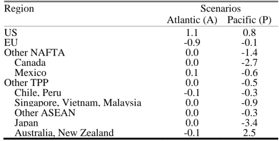
In terms of agri-food output, the pattern is similar for both agreements. While US agri- food production increases, in almost all other countries production contracts (Table 7).
The Pacific agreement entails moderate losses for most countries except Canada (-2.7%), which suffers from an erosion of its existing preferential access (due to both initial preferences and the NAFTA Agreement) to the US. Japanese production also faces a decline (-3.4%) concentrated in a few sectors (fruits and vegetables, beverages and tobacco, and other food) where Australia, New Zealand, and the US have strong comparative advantages. Due to this comparative advantage, output related to agri-food for Australia and New Zealand benefits from the Pacific agreement (+2.5%). New Zealand also gains from the opening of the Japanese and Canadian dairy markets which currently are very protected (respective initial tariffs are 99% and 142%). This last result is also found by Burfisher et al. (2014).
The Atlantic agreement scenario results in a decrease in European agri-food production (-0.9%). Thus, for the EU, the increase in trade flows is countered by the decrease in intra- EU trade entailed by the agreement. Table 7 shows that the Atlantic agreement has little impact on the output of Pacific countries and vice versa.
Table 7: Variation in agri-food output, 2025 (percentage change in volume)
Region Scenarios
Atlantic (A) Pacific (P)
US 1.1 0.8 EU -0.9 -0.1 Other NAFTA 0.0 -1.4 Canada 0.0 -2.7 Mexico 0.1 -0.6 Other TPP 0.0 -0.5 Chile, Peru -0.1 -0.3
Singapore, Vietnam, Malaysia 0.0 -0.9
Other ASEAN 0.0 -0.3
Japan 0.0 -3.4
Australia, New Zealand -0.1 2.5
Note: Authors’ calculations.
4.2. Differences in the sector issues at stake lead to almost no competition between the agreements
As initial sector protection varies (in terms of tariffs and NTMs), the impacts of the Pacific and Atlantic agreements are dissimilar across sectors. Our CGE simulations allow us to highlight the offensive and defensive sectors for TPP and TTIP member countries. The classification of these sectors is based on the expected sign of the variation in production. More precisely, if a country is likely to face a positive (respectively negative) variation in production in a given sector following the agreement’s implementation, then this sector represents an offensive (respectively defensive) interest for that country. The offensive/defensive features are largely based on countries’ initial sector competitiveness and potential complementarities with trading partners. Figure 1 compares the variation in agri-food production induced by both agreements. Coordinates on the horizontal axis denote the variation in output (pct. points) due to the Atlantic
20
agreement, while coordinates on the vertical axis denote the variation in output due to the Pacific agreement. The size of the bubbles denotes the size of value-added in the BAU scenario. At sector level, white meat, cereals, other animal products, fruits and vegetables, and other food constitute US offensive sectors under both agreements, while red meat and live animals represent an offensive interest only in the Atlantic agreement scenario. The US also has some defensive sectors: dairy, vegetable oils, beverages and tobacco in the Atlantic case, and sugar cane in the Pacific scenario (although this sector does not represent a large share of US agri-food production).
The Atlantic scenario has a negative impact on EU production especially in animal products (especially red meat: -8.6%), while vegetable oils, and beverages and tobacco exhibit an increase. These results are in line with Erixon and Bauer (2010), Fontagné et al. (2013) and Beckman et al. (2015) who also highlight the sensitivity of beef meat and vegetal oils in each side of the Atlantic in case of TTIP Agreement. It is worth noting that the Pacific agreement only has an effect on European white meat production due to the competition from Australia and New Zealand in the US market. However, this variation is very small (-0.5%). Our results on the variation in agri-food production in the Atlantic scenario are somewhat different from those obtained by Francois et al. (2013), who find an increase in EU value added and a decrease for the US. These differences mainly lie in the method used for the computation of the AVEs of NTMs and in the level of sector disaggregation. In Francois et al. (2013), agriculture is disaggregated into two different sectors only (against 16 in our case), hence hiding huge heterogeneity. This heterogeneity drives our results: US comparative advantages are in sectors impacted by stringent NTMs in the EU (red and white meat, dairy products) – and hence facing a relative high decrease in trade costs in the Atlantic scenario –, while EU best performing sectors (dairy, other food products, and beverages and tobacco) are not affected by strong NTMs in the US.
In the Pacific agreement scenario, Canada and Mexico are the most affected countries. In the case of both countries, output in the red and white meat sectors is positively impacted, while the dairy sector is negatively affected. Note however that these sectors are rather small in size. The picture is reversed for other TPP countries, where the dairy sector represents an offensive interest (mainly for New Zealand), and the white and red meat output is decreasing. Lastly, TPP countries’ production in these sectors is affected by the Atlantic agreement, but the impact is limited (less than 0.3%). Our results are relatively similar to Burfisher et al. (2014), who show that US output will increase in most agri-food sectors due to an increased market access within the TPP area. Burfisher et al. (2014) also emphasize the gains in the dairy sector for New Zealand.
Given the sector specializations of countries involved in both agreements, the competition effects between the EU and Pacific products on the US market are likely to be unimportant even were both agreements to be implemented simultaneously. However, since US offensive interests are the same in both the TPP and TTIP markets, it is possible that a saturation of US production would be observed. In that case, trade (and welfare) gains would be lower than the sum of the gains stemming from the Atlantic-only and Pacific-only scenarios.
21
Figure 1: Comparative variation in agri-food output (pct. variation) and initial agri-food value-added (million 2007 USD) for TTIP and TPP countries, 2025
Note: Authors' computation. Coordinates on the horizontal axis denote the variation in output (pct. points) due to the Atlantic agreement, while coordinates on the vertical axis denote the variation in output due to the Pacific agreement. The size of the bubbles denotes the size of value-added in the BAU scenario. Scales differ from one panel to the next. Dotted lines represent the first bisector (along which the impact is the same over the two agreements).
22
From a broader point of view, our results also show that the impact of each agreement on its signatories’ real income – the purchasing power part of welfare – is positive but very limited
(around 0.1%).19
4.3. Third countries may be impacted by both agreements
We first investigate the impact of the Atlantic and Pacific agreements on third countries’ overall agri-food production (Table 8). Potential TPP members with the exception of the group of Other Latin American countries are almost unaffected. Similarly, Eastern European, Middle-Eastern and African countries would not suffer significantly from the conclusion of the Atlantic or Pacific agreement. However, the Latin American countries (especially Brazil and Argentina) and the EFTA countries which historically are partners of the US and the EU, would face competition in their export markets following the implementation of the TPP and TTIP Agreements, which is also highlighted by Beckman et al. (2015). The reduction in output incurred by these countries is relatively high (respectively -0.4% for Argentina, -0.5% for Brazil, and -0.6% for the EFTA countries) compared to the losses (less than 0.1%, see Table 7) that would be suffered by the EU, and TPP countries being excluded respectively from the TPP and TTIP Agreements.
Figure 2 depicts the impact of both the Atlantic and Pacific agreements on Argentina, Brazil, and the EFTA countries’ output at sector level. For the majority of sectors, the variation in production is small (around 0.1%). Therefore, the losses in total agri-food production highlighted previously in fact are driven by a few sectors. In Brazil, the white meat and other animal products sectors are affected by both agreements. In addition, an Atlantic agreement would entail some risks for the cereals, red meat and live animals sectors (based on decreased meat production in that country). The picture for Argentina is similar to the Brazilian sectors due to the comparable sector specializations in these two countries. However, the Pacific agreement would affect Argentina less than Brazil because the TPP countries represent a smaller share of its exports.
19 Real income encompasses the variations in the representative agent's revenue and the changes in the prices of
goods. However, since the model relies on perfect competition (no profit) and full employment of production factors (no unemployment), and given the assumptions on the modelling of NTMs (see Section 3.1), the welfare impacts of both the Atlantic and Pacific agreements cannot be analysed using the real income results. These income results are nevertheless available upon request.
23
Table 8: Variation in third countries’ agri-food output, 2025 (percentage change)
Region Scenarios
Atlantic (A) Pacific (P) A/P
Potential TPP members 0.0 0.0 -0.1
China 0.0 0.0 0.0
India 0.0 0.0 -0.1
Korea 0.1 0.0 0.1
Other Asia 0.0 0.0 -0.1
Other Latin America -0.2 -0.1 -0.3
Third countries -0.1 -0.1 -0.2 Argentina -0.3 -0.1 -0.4 Brazil -0.3 -0.2 -0.5 EFTA -0.2 -0.4 -0.6 Russia 0.0 -0.1 -0.1 Other Europe -0.1 0.0 -0.1 Turkey 0.0 0.0 0.0
Other Middle East -0.1 0.0 -0.1
North Africa -0.1 0.0 -0.1
Sub-Saharan Africa 0.0 0.0 -0.1
Note: A/P stands for Atlantic and Pacific agreements simultaneously. Source: authors’ calculations.
Both agreements affect the agri-food sectors in EFTA countries. Among these countries, Switzerland is strongly affected, due to its specialization in dairy, chocolate and preparations. Impacts are higher in case of the Pacific agreement. Although EU is the main partner of EFTA countries, products exported by EFTA to the EU (other food products for Switzerland, fish for Norway) would not have to compete with important flows coming from the US in the case of an Atlantic agreement. However, the US is the second most important market (after the EU) for EFTA, milk and dairy exports (especially for Switzerland), and the third market for other food (after the EU and Russia). Thus, EFTA access to the US market would be affected by a Pacific agreement and would lead to reductions in output.
24
Figure 2: Comparative variation in agri-food output (pct. variation) and initial agri-food value-added (million 2007 USD) for third countries, 2025
25
4.4. Sensitivity analysis
In this section, we investigate the sensitivity of our results to alternative assumptions.
4.4.1. No significant cross-agreement interactions if both are implemented
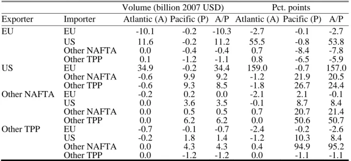
Table 9 reports the variation in agri-food trade by importer and exporter, in the Atlantic only scenario “A”, in the Pacific only scenario “P”, and in the simultaneous introduction scenario (“A/P”). Indeed, the Atlantic and Pacific agreements are likely to come into force simultaneously. Comparison of trade variations across scenarios suggests few interactions between agreements. If both agreements are implemented simultaneously, the competition between EU and TPP exporters in the US market could reduce the trade gains of these two groups compared to the scenarios with only one agreement. On the US side, since the US exports quite similar products to the EU and the TPP countries, the “A/P” scenario could result in saturation of production in the US. This would reduce US export capacity and lead to less export creation than in the Atlantic or Pacific only scenarios. This would thus leave more room for intra-regional trade (intra-EU and intra-TPP, US excepted).
All these effects appear in Table 9, though with limited magnitude: production in the US turns out to be relatively elastic, while the EU and other TPP countries do not penetrate the US market with the same goods.
Table 9: Variation in agri-food trade compared to BAU, 2025 (exports in billion 2007 USD at constant FOB price and percentage change)
Volume (billion 2007 USD) Pct. points
Exporter Importer Atlantic (A) Pacific (P) A/P Atlantic (A) Pacific (P) A/P
EU EU -10.1 -0.2 -10.3 -2.7 -0.1 -2.7 US 11.6 -0.2 11.2 55.5 -0.8 53.8 Other NAFTA 0.0 -0.4 -0.4 0.7 -8.4 -7.8 Other TPP 0.1 -1.2 -1.1 0.8 -6.5 -5.9 US EU 34.9 -0.2 34.4 159.0 -0.7 157.0 Other NAFTA -0.6 9.9 9.2 -1.2 21.9 20.5 Other TPP -0.6 9.3 8.5 -1.8 26.7 24.4 Other NAFTA EU -0.2 0.2 0.0 -2.1 2.1 -0.1 US 0.0 3.6 3.5 -0.1 8.7 8.4 Other NAFTA 0.0 0.5 0.5 0.7 20.7 21.4 Other TPP 0.0 6.2 6.2 0.0 50.6 50.7 Other TPP EU -0.7 -0.1 -0.7 -2.4 -0.2 -2.6 US -0.2 1.8 1.4 -1.2 10.3 8.4 Other NAFTA 0.0 4.3 4.3 0.4 94.9 95.2 Other TPP 0.0 -1.2 -1.2 0.0 -1.1 -1.1
Note: Authors’ calculations. A/P stands for Atlantic and Pacific agreements simultaneously.
As previously emphasized, much uncertainty remains around the content of the future Atlantic and Pacific agreements. In the following two subsections, we test the sensitivity of our results to different negotiation outcomes.