The EUA-sCER Spread: Compliance Strategies and Arbitrage in the European Carbon Market

HAL Id: halshs-00458991

https://halshs.archives-ouvertes.fr/halshs-00458991

HAL is a multi-disciplinary open access archive for the deposit and dissemination of sci-entific research documents, whether they are pub-lished or not. The documents may come from teaching and research institutions in France or

L’archive ouverte pluridisciplinaire HAL, est destinée au dépôt et à la diffusion de documents scientifiques de niveau recherche, publiés ou non, émanant des établissements d’enseignement et de recherche français ou étrangers, des laboratoires

Arbitrage in the European Carbon Market

Maria Mansanet-Bataller, Julien Chevallier, Morgan Hervé-Mignucci, Emilie

Alberola

To cite this version:

Maria Mansanet-Bataller, Julien Chevallier, Morgan Hervé-Mignucci, Emilie Alberola. The EUA-sCER Spread: Compliance Strategies and Arbitrage in the European Carbon Market. 2010. �halshs-00458991�

•

N°

2010

–

6

The EUA-sCER Spread: Compliance Strategies

and Arbitrage in the European Carbon Market

Maria Mansanet-Bataller

, Julien Chevallier

,

Morgan Hervé-Mignucci

, and Emilie Alberola

First Version: January 13, 2010

Abstract:

This article studies the price relationships between EU emissions allowances (EUAs) – valid under the EU Emissions Trading Scheme (EU ETS) – and secondary Certified Emissions Reductions (sCERs) – established from primary CERs generated through the Kyoto Protocol’s Clean Development Mechanism (CDM). Given the price differences between EUAs and sCERs, financial and industrial operators may benefit from arbitrage strategies by buying sCERs and selling EUAs (i.e. selling the EUA-sCER spread) to cover their compliance position between these two assets, as industrial operators are allowed to use sCERs towards compliance with their emissions cap within the European system up to 13.4%. Our central results show that the spread is mainly driven by EUA prices and market microstructure variables and less importantly, as we would expect, by emissions-related fundamental drivers. This might be justified by the fact that the EU ETS remains the greatest source of CER demand to date.

Keywords: EUA-sCER Spread; Arbitrage; Emissions Markets.

* _{Corresponding author. Mission Climat - Caisse des Dépôts, Paris, France. maria.mansanet@caissedesdepots.fr} † _{Université Paris-Dauphine (CGEMP/LEDa), Imperial College London (Grantham Institute for Climate Change), and}

Working papers are research materials circulated by the authors for purpose of information and discussions. They have not necessarily undergone formal peer review. The authors take sole responsibility for any errors or omissions.

Table of Contents

1.Introduction ... 4

2.Compliance Strategies in the EU ETS... 7

2.1. EUAs and CERs contracts 7 2.2. Price development 8

3.Cointegration Analysis... 10

3.1. Unit Roots and Structural Break 10 3.2. VECM and Structural Break 11 3.3. VAR(p) Modeling 12

4.EUAs Price Drivers ... 14

4.1. Database 15 4.2. GARCH Modeling 20 4.3. Estimation results 20

5.sCER Price Drivers ... 22

5.1. Exogenous variables 22 5.2. GARCH modeling 24 5.3. Estimation results 24

6.EUA-sCER Spread drivers... 26

6.1. Exogenous variables 27 6.2. GARCH modeling 31 6.3. Estimation results 31

7.Conclusion... 35

Acknowledgements... 36

References ... 37

1. Introduction

The European Union Emissions Trading Scheme (EU ETS) is the EU's flagship climate policy forcing industrial polluters to reduce their CO2 emissions in order to help the

European Member States to achieve their Kyoto Protocol target (i.e. to reduce greenhouse gas emissions on average by 8% with respect to 1990 levels). As an emissions cap, industrial operators receive, in Phases I (2005-2007) and II (2008-2012) of the scheme, a yearly allocation of European Union Allowances (EUAs), which represent the right to emit one ton of CO2 in the atmosphere.1 The compliance of industrial operators requests the

balance between verified emissions and allocated allowances. Besides, industrial operators may cut the costs of reducing their emissions by using credits issued from the Kyoto Protocol Clean Development Mechanism (CDM), called Certified Emissions Reductions (CERs).2 These CERs correspond to one ton of avoided CO2 emissions in the atmosphere,

and may be obtained through projects development in non Annex-B countries of the Kyoto Protocol that allow to reduce emissions compared to a baseline scenario. Once credits have been issued by the United Nations’s CDM Executive Board they may be sold by project developers on the market, and thus become secondary CERs (sCERs). The central goal of this article is to study the price drivers of EUAs and sCERs, and to explain the evolution of the price difference observed between these two assets (the EUA-sCER spread).

Even if both assets allow the emission of one ton of CO2 in the atmosphere, we observe

the existence of a positive spread between EUA and sCER prices that may be due to the partial fungibility between these two carbon assets. Indeed, to provide more flexibility to carbon-constrained installations, the European Commission has allowed industries covered by the EU ETS to use both assets for compliance. However, it has established a limit on the use of CERs (primary or secondary) up to 13.4% of their allocation from 2008 to 2012 on average. To comply with their emissions cap, industrial emitters may thus adopt various strategies: (i) surrender EUAs (allocated either to the plant or to others plants of the same company), (ii) reduce real emissions (either at the installation-level or abroad, using the Kyoto Protocol’s flexibility mechanisms), (iii) buy EUAs or/and sCERs, (iv) borrow EUAs from future allocation, (v) surrender banked EUAs from past allocation. Trotignon and Leguet (2009) document that, in 2008, 96% of the surrendered allowances were EUAs, and only 3.9% were sCERs.3 _{The trade-offs between using EUAs or sCERs towards compliance}

1 _{For Phase III of the EU ETS starting in 2013, the main part of EUAs will be allocated to industrials though} auctioning. The power sector will have to buy 100% of its allocation, while sectors faced to international competition and some carbon leakages will keep receiving a free yearly allocation.

2 _{Emission Reduction Units (ERUs) generated through the Joint Implementation mechanism (JI) of the Kyoto} Protocol fall beyond the scope of this article, and are left for future research.

3 _{Note 0.01% were ERUs. No CERs were used towards compliance before that period, due to the lack of} connection between the Kyoto Protocol’s International Transaction Log (ITL) and the EU ETS’ Community Independent Transaction Log (CITL).

in the EU ETS depend on the limit of CERs which can be used for compliance, their respective price trends, and the price difference between them. Carbon traders and brokers are following closely the evolution of the EUA-sCER spread, which reflects the uncertainties embedded in the development of both schemes.In theory, as the sCERs are free of project delivery risks, the prices of EUAs and sCERs should be equal since they represent the same amount of CO2 emissions reduction (one ton). However, due to the limit

of 13.4% on average of the credits surrendered, the sCERs’ “exchange rate” is smaller than for EUAs, and therefore sCERs are discounted with respect to EUAs. This premium represents the opportunity cost of using sCERs for compliance instead of EUAs.

Beyond prices, regulatory issues may also explain the variation of the spread between these two carbon assets in the long run. First, with the European Energy Climate package, the EU ETS is confirmed until 2020. However, the details concerning the import of CDM credits within Phase III (2013-2020) are not known with certainty. Indeed, the European Union establishes particular conditions of the emissions trading scheme in Phase III that are dependent on the achievement of a post-Kyoto international agreement. Thus, there exists a wide range of uncertainties arising around the status and recognition of CERs (both primary and secondary) in a revised EU ETS beyond 2012. Second, carbon assets form another class of commodities against which traders need to define specific hedging strategies (Chevallier (2009), Chevallier et al. (2009)).

The existence of spreads between assets has been studied mainly on financial markets. Collin-Dufresne et al. (2001) find that credit spread changes in the U.S. are mainly driven by local supply and demand shocks. Manzoni (2002) characterizes the evolution of credit spreads on the sterling Eurobond market by a cyclical behavior and persistent volatility process. Zhang (2002) examines the predictive power of credit spreads from the corporate bond market in the U.S., and supports Bernanke and Gertler’s (1989) credit channel theory as the explanation for the strong forecasting ability of credit spreads. Codogno et al. (2003) show that differentials between Euro zone government’s bond spreads may be explained by banking and corporate risk premiums in the U.S. Ramchander et al. (2005) investigate the influence of macroeconomic news on interest rates and yield spreads in the U.S. and they find that Consumer Price Index, non-farm payroll figures, and Fed funds rate release announcements have a significant influence on changes in these spreads. Gómez-Puig (2006) highlights the importance of size and liquidity indicators in explaining sovereign yield spreads following the European Monetary Union. Davies (2008) examines U.S. credit spread determinants with an 85 year perspective. Based on cointegration techniques for the determinants of credit spreads, he demonstrates that key causal relationships exist independently across different inflationary environments. Liu and Zhang (2008) investigate whether the value spread is a useful predictor of returns. They identify mixed evidence, as two related variables, the book-to-market spread (the book-to-market of value stocks minus

opposite signs. Manganelli and Wolswijk (2009) further study the spreads between Euro area government’s bond yields, and find that they are related to short-term interest rates, which are in turn related to liquidity risk components.

Compared to previous literature, we provide the first empirical analysis of EUA and sCERs drivers, and the determinants of the EUA-sCER spread during Phase II (2008-2012) of the EU ETS. Mansanet-Bataller et al. (2007), Alberola et al. (2008), and Alberola and Chevalier (2009) have already analyzed the price fundamentals of EUAs during Phase I (2005-2007) of the EU ETS, but not the drivers of EUAs or sCERs during Phase II. Additionally, to our best knowledge, no previous empirical study has focused either on the determination of sCERs drivers or on the arbitrage strategies consisting in buying sCERs and selling EUAs (yielding net profits from the existence of the positive EUA-sCER spread).

Our central results show that EUAs and sCERs share the same price drivers, i.e. these emissions markets prices are mainly determined by institutional events, energy prices, weather events, and macroeconomic variables. Moreover, EUAs are found to determine significantly the price path of sCERs, by accounting for a large share of the explanatory power of sCERs prices. This result emphasizes that EUAs remain the main “money” in the field of emissions market, which is exchanged broadly as the most liquid asset for carbon trading. The trading of sCERs, while growing exponentially, is still mostly determined by the fact that the EU ETS remains the largest emissions trading scheme to date in the world.4

This result also explains why sCERs are traded at a discounted price from EUAs: absent the project risk which is characteristic of primary CERs, sCERs are still limited by the import limit set within the EU ETS.

Regarding the EUA-sCER spread, our central contribution documents that variables stemming from the market microstructure literature (such as volumes exchanged on each emissions market, see Madhavan (2000) for a review) are the main drivers of the spread, in addition to EUA price levels, institutional and macroeconomic variables, and forecast errors on the delivery of primary CERs. The latter result may indicate that the EUA-sCER spread is traded as a “speculative” product by market participants such as traders and energy utilities companies, since it is possible to obtain a net benefit by simultaneously trading EUAs and sCERs (when the price difference between these two assets is above a certain profitability threshold). Taken together, our results indicate that while the fungibility between emissions markets worldwide is quickly developing, there remain significant opportunities for price arbitrage.

The remainder of the article is organized as follows. Section 2 details compliance strategies in the EU ETS. Section 3 develops a cointegration analysis between EUAs and

4 _{Note that this situation could change with the future developments from the U.S. federal cap-and-trade} scheme and other regional initiatives.

sCERs prices. Section 4 reviews the main EUAs price drivers. Section 5 covers the specific sCERs price drivers. Section 6 focuses on the determinants of the EUA-sCER spread. Section 7 summarizes the article with some concluding remarks.

2. Compliance Strategies in the EU ETS

This section briefly reviews background information on the EU ETS, which was launched in 2005 according to the Directive 2003/87/EC to facilitate the EU compliance with its Kyoto commitments. Phase I was introduced as a training period during 2005-2007. Phase II coincides with the commitment period of the Kyoto Protocol (2008-2012). Phase III will cover the period 2013-2020. Around 11,000 energy-intensive installations are covered by the scheme, which accounts for nearly 50% of European CO2 emissions

(Alberola et al., 2009a, 2009b). Emissions caps are determined at the installation-level in National Allocation Plans (NAPs). In what follows, we examine more closely EUAs and CERs contracts, as well as their respective price developments.

2.1. EUAs and CERs contracts

On the one hand, EUAs are the default carbon asset in the EU emissions trading system. They are distributed by European Member States throughout NAPs, and allow industrial owners to emit one ton of CO2 in the atmosphere. The supply of EUAs is fixed in NAPs,

which are known in advance by market participants (2.08 billion per year during 2008-2012).5

On the other hand, CERs, which also compensate for tons of CO2 emitted by their

owners, are much more heterogeneous than EUAs. Primary CERs represent greenhouse gases emissions reductions achieved in non-Annex B countries of the Kyoto Protocol. These certificates are issued by the United Nations Clean Development Mechanism Executive Board (CDM EB). CDM projects may associate various partners (ETS compliance buyers, Kyoto-bound countries, project brokers, profit-driven carbon funds, international organizations such as the World Bank, etc.). CDM projects partnerships are governed by emissions reduction purchase agreements (ERPAs).6 _{The price of primary}

CERs will depend on the risk of each project, and on its capacity to effectively issue

5 _{However on September 23, 2009, the European Court of First Instance (CFI) overruled the decision of the} European Commission concerning NAPs for the second period submitted by Estonia and Poland. The Commission will explore two options: (1) issue a new decision based on “proper” criteria before December 23, 2009; and (2) appeal the CFI ruling, on a point of law, before November 23, 2009. Six other Eastern European countries may contest NAPs as well. In total, it represents a potential additional 162 million allowances.

primary CERs. This price will be the cost of the project divided by the number of primary CERs actually issued. Thus, primary CERs from different projects will have different prices.

Once issued by the CDM EB, primary CERs may either be used by industrial firms for their own compliance, or sold to other participants in the market. In the latter case, it becomes a secondary CER (sCER). Note that as the sCERs are CERs that have been already issued by the CDM EB, their project delivery risk is null. As stated in the introduction, the main difference between the use of EUAs and CERs (including both, primary and secondary) for compliance in the EU ETS lies in the 13.4% (on average) import limit set by the European Commission on CERs, while EUAs may be used without any limit. The CERs import limit for compliance is equal to 1.4 billion tons of offsets being allowed into the EU ETS from 2008-2012.7

In this article we focus on the price relationships between EUAs and sCERs. Next, we describe the EUAs and sCERs price developments.

2.2. Price development

In this section, we examine Phase II EUA and sCER prices, which reflect the price of reducing emissions during the commitment period of the Kyoto Protocol (2008-2012).8 The sCER price series used for this study is the longest historical price series existing for sCERs: the sCER Price Index developed by Reuters. It has been built by rolling over two sCERs contracts with different maturity dates (December 2008 and December 2009). Similarly, we have rolled over EUA futures contracts traded at the European Climate Exchange (ECX) of the corresponding maturity dates (December 2008 and December 2009) to match them with the sCER price series.9 _{The sample period considered starts with}

the beginning of the sCER Price Index (March 9, 2007) and ends on March 31, 2009. As shown in Figure 1, the EUA and the sCER price series follow a similar price path.

7 _{In the absence of a satisfactory international agreement, installations subject to allowances during Phase III} will only be able to use the credits left over from Phase II (2008-2012), or a maximum amount corresponding to 11% of the Phase II allocation. These measures are equivalent to capping the potential demand for Kyoto credits to 1,510 Mt between 2008 and 2020. If a post-Kyoto international agreement is achieved, the ceiling on the use of credits from project mechanisms towards the compliance of EU ETS installations will be raised to 50% of the additional reduction efforts. Beyond this issue, the introduction of a new international agreement on climate change would introduce “high quality” as a condition for project credits coming from countries which have signed the international agreement. This would translate into a reduced supply of credits originated from project mechanisms to EU ETS compliance buyers.

8 _{Note that banking and borrowing of allowances are allowed within Phases II and III of the EU ETS, contrary} to Phases I and II (Alberola and Chevallier (2009)).

9 _{Carchano and Pardo (2009) analyse the relevance of the choice of the rolling over date using several} methodologies with stock index future contracts. They conclude that regardless of the criterion applied, there are not significant differences between the series obtained.

EUAs were traded at €15 in March 2007, then stayed in the range of €19-25 until July 2008, and decreased steadily afterwards to achieve €8 in February 2009. sCERs started at €12.5 in March 2007, evolved in the range of €12-22 through July 2008, and continued to track EUA prices until €7 in February 2009. Thus, sCERs have always remained below EUAs and consequently the spread has been positive during all the sample period.

Figure 1: Time-series of ECX EUA Phase II Futures, Reuters CER Price Index, and CER-EUA Spread from March 9, 2007 to March 31, 2009

0 5 10 15 20 25 30 35 09/03/2007 09/07/2007 09/11/2007 09/03/2008 09/07/2008 09/11/2008 09/03/2009 Eu ro s

EUA CER Spread

Source: Reuters

Descriptive statistics for EUAs, sCERs, and the spread may be found in Table 1. Given the price paths observed in historical data, it appears interesting to investigate the presence of one cointegrating relationship between EUAs and sCERs in the next section.

Table 1: Summary statistics for all dependent variables

Variable Mean Median Max Min Std. Dev Skew. Kurt

Raw Prices series

EUAt 20.40389 21.52000 29.33000 8.20000 4.459218 -0.765966 3.031938 sCERt 15.85798 16.6875 22.8500 7.484615 2.986495 -0.351494 3.135252 Spreadt 4.545912 4.620000 9.043571 0.647857 2.108445 0.047792 2.292397 Nathural Logarithms EUAt 2.986643 3.068983 3.378611 2.104134 0.255164 -1.323179 4.275898 sCERt 2.743941 2.776476 3.128951 2.012850 0.505511 -0.994736 4.182189 Log returns EUAt -0.000437 0.0001 0.113659 -0.094346 0.026833 -0.060828 4.868026 sCERt -0.000309 0.0001 0.112545 -0.110409 0.024441 -0.370323 5.961950 VAR(4) Residuals EUAt 0.00001 0.001242 0.108251 -0.094873 0.05903 -0.052333 4.522629 sCERt 0.00001 0.000390 0.111584 0.097672 0.023742 -0.309379 5.520998 First-differences Δ Spread -0.002219 -0.010179 1.070000 -1.740000 0.295605 -0.368420 6.262861

Note: EUAt refers to ECX EUA Futures, sCERt to Reuters sCER Price Index, and Spreadt = EUAt-sCERt spread. Std.Dev. stands for Standard Deviation, Skew. for Skewness, and Kurt. for Kurtosis. The number of observations is 529. The VAR(4) specification is detailed in Section 2.3.

3. Cointegration Analysis

Following the methodology used in Manzoni (2002) and Ramchander et al. (2005), who studied the relationship between bond spreads, we proceed in a first step by identifying the possible cointegration relationship between the two types of assets considered (EUAs and sCERs). We will then analyze the EUA-sCER spread drivers.

3.1. Unit Roots and Structural Break

A necessary condition for studying cointegration involves that both time-series are integrated of the same order. We thus examine the order of integration, noted d, of the time-series under consideration based on Zivot and Andrews’ (1992) unit root test. This test allows examining the unit root properties of the time-series, while simultaneously detecting endogenous structural breaks for each variable. Figure 2 presents the Zivot-Andrews unit root test statistics for the two EUA and sCER variables transformed to log-returns.

Figure 2: Zivot-Andrews (1992) Test Statistic for the EUA (left) and sCER (right) Variables

The model estimated is a combination of a one-time shift in levels, and a change in the rate of growth of the series. The null of unit root is clearly rejected in favour of the break-stationary alternative hypothesis. One estimated break point is identified for each of the time-series: February 13, 2009 for the EUA variable, and February 20, 2009 for the sCER variable. These breakpoints may be due to a delayed effect of the “credit crunch” crisis on the carbon market (see Chevallier (2009) for a discussion). Both time-series are integrated of order 1 (I(1)). The existence of a structural break in the time-series considered, while

remaining stationary, means that we need to develop cointegration tests that explicitly include potential breaks, as they have been developed by Lutkepohl et al. (2004).

3.2. VECM and Structural Break

After having validated the necessary condition for studying cointegration (which involves that both time-series should be integrated of the same order), we investigate the existence of a long-term relationship across these two carbon prices by employing a cointegration analysis with the maximum-likehood test procedure established by Johansen and Juselius (1990) and Johansen (1991). Results for the cointegration test with one structural shift at unknown time (Lutkepohl et al (2004)) are shown in Panel A of Table 2. The trace statistic result indicates a cointegration space of r = 1, given a 5% significance level. We may conclude that there exists one long-term cointegrating vector between the EUA and sCER variables taken in natural logarithm form.

Table 2: Johansen Cointegration Rank Trace Statistic, Cointegration Vector, Model Weights and VECM with Structural Break for the EUA and the CER Variables.

Panel A: Johansen Cointegration Rank Trace Statistic

Hypothesis Statistic 10% 5% 1% 1

≤

r 5.26 5.42 6.79 10.04

r = 1 16.95 13.78 15.83 19.85

Panel B: Cointegration Vector

Variable EUA (1) sCER (1)

EUA (1) 1.0000 1.0000

sCER (1) -0.4955009 -1.519945

Panel C: Model Weights

Variable EUA (1). sCER (1)

ΔEUA -0.06163548 0.00734759

ΔsCER -0.04490726 0.0182197

Panel D: VECM with Structural Break (r = 1)

Variable ΔEUA ΔsCER

Error Correction Term (ect) -0.0197908 -0.0282009

Deterministic constant 0.0106349 0.0154190

Lagged differences

ΔEUA (1) -0.0641515 -0.0504123

ΔsCER (1) 0.2307197 0.1423340

Note: EUA refers to ECX EUA Phase II Futures, sCER to Reuters sCER Price Index, transformed to natural logarithms. Critical values are reported in Lutkepohl et al (2004). Lag order in parenthesis. The number of observations is 529.

Next, we proceed to the estimation of the Vector Error Correction Model (VECM), which is useful in making causal inferences among the variables of our system.10 _{As shown}

in Panel D of Table 2, the coefficients of the error correction terms for the EUA and sCER variables are negative, and thus we validate the error correction specification. In terms of short-run dynamics, the error correction terms emerge as important channels of influence in mediating the relationship between the different EUAs and sCERs prices. We notice in Panel D of Table 2 that the error correction term appears stronger for sCERs than for EUAs. This implies that the sCER variable has a stronger behavior to adjust to past disequilibria by moving towards the trend values of the EUA variable. This specification confirms that EUAs constitute a leading factor in the price formation of sCERs. It can also be seen that changes in the respective prices of EUAs and sCERs have a significant causal influence (in the Granger sense) on each other.11

3.3. VAR(p) Modeling

In light of the previous results, and in order to proceed with the suitable identification of the price drivers for each variable, we use a VAR(p) in differences with an intervention dummy for February 2009 to model the data-generating process of the EUA and sCER log-series. The VAR(p) model is specified as follows:

ε + Δ + + Δ + Δ + = Δyt A0 A1 yt−1 A2 yt−2 ... Ap yt−p Where _⎥ ⎦ ⎤ ⎢ ⎣ ⎡ Δ Δ = Δ t t t sCER EUA

y is a vector of EUA and sCER log-returns, _⎥

⎦ ⎤ ⎢ ⎣ ⎡ = 20 10 0 b b A is a vector of constants, and _⎥ ⎦ ⎤ ⎢ ⎣ ⎡ = 22 12 21 11 1 _γ γ γ γ

A , etc. are the coefficient matrices.

To determine the appropriate lag structure, we computed the following information criteria: Akaike (AIC(n)=4), Schwarz (SC(n)=1), Hannan-Quinn (HQ(n)=1), and Final Prediction Error (FPE(n)=4). Since the Ljung-Box-Pierce Portmanteau test on the residuals

10 _{The VECM is specified as follows:} ε + Δ + + = Δyt A0 A1Ecmt−1 A2 yt−1 Where _⎥ ⎦ ⎤ ⎢ ⎣ ⎡ Δ Δ = Δ t t t _sCER EUA

y is a vector of first differences of EUA and sCER prices, _⎥

⎦ ⎤ ⎢ ⎣ ⎡ = 20 10 0 _b b A is a vector of constants, _⎥ ⎦ ⎤ ⎢ ⎣ ⎡ = 21 11 1 b b

A is a vector measuring the speed of the adjustment to the long-run relationship,

and _⎥ ⎦ ⎤ ⎢ ⎣ ⎡ = 22 12 21 11 2 _γ γ γ γ A is a coefficient matrix.

of the VAR(1) model indicated the presence of autocorrelation, we choose to retain a lag of order p = 4. As shown in Table 3, residuals are not auto-correlated for the VAR (4) model.

Table 3: Diagnostic test of VAR(4) Model

Test Statistic D. F. p-value

Portmanteau 57.4878 48 0.16

ARCH VAR 97.1946 9 0.01

JB VAR 147.6817 4 0.01

Kurtosis 143.5005 2 0.01

Skewness 4.1811 2 0.12

Note: Portmanteau is the asymptotic Portmanteau test with a maximum lag of 16, ARCH VAR is the multivariate ARCH test with a maximum lag of order 5, JB is the Jarque Bera Normality test for multivariate series applied to the residuals of the VAR(4). Kurtosis and Skweness stand for separate tests for multivariate skewness and kurtosis. D.F. stands for degree of freedom of the test statistic.

The ARCH effect is very strong, which indicates the necessity to use a GARCH model for further analysis. Figure 3 plots the log-returns and the VAR(4) residuals of the ECX EUA Phase II Futures and sCER Price Index time price series.

Figure 3: Log-returns (left) and VAR(4) residuals (right) of ECX EUA Phase II Futures and Reuters sCER Price index for the sample period from March 9, 2007 to March 31, 2009

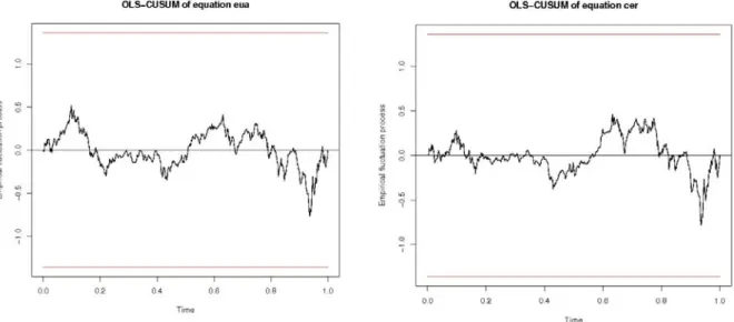
Figure 4 shows the OLS-based CUSUM tests for the VAR (4) residuals. Despite some structural instability around the February 2009 breakpoints, the residuals stay within the interval confidence levels.

Figure 4: OLS-CUSUM Test for the EUA (left) and sCER (right) Variables of the VAR(4) Model

Additional impulse response analysis reveals the traditional “hump” shape between EUAs and sCERs, as shocks pass on both variables and fluctuations dampen at the horizon of 10 lags.12 _{The variance decomposition indicates that the variance of the forecast error for}

the EUA price is due to its own innovations up to 90%. For the sCER price, the variance of the forecast error is due to EUAs up to 70%, and only 30% to its own innovations. These results confirm our findings in Section 2.2.

In the next step of our empirical analysis, we proceed by fitting a suitable GARCH model to the residuals of the VAR (4) model for the EUA and sCER variables.

4. EUAs Price Drivers

In this section, we focus on the drivers of EUAs using the residuals of the VAR(4) model. As detailed in previous literature, we may distinguish between factors determining the supply and demand of EUAs. The supply of EUAs is fixed by the European Commission in National Allocation Plans that are validated after negotiation between Member States and national industrials covered by the scheme. Announcements relative to the strictness of NAPs have been shown to have a strong influence on EUA prices (Alberola et al. (2008), Chevallier et al. (2009), Mansanet-Bataller and Pardo (2009)). Concerning demand factors, previous literature identifies energy prices, weather events, and the level of industrial production as being the main drivers of EUAs during Phase I (Mansanet-Bataller et al. (2007), Alberola et al. (2009a, 2009b).

4.1. Database

We include as EUAs price drivers the most representative energy prices in Europe. That is, the daily Brent and natural gas futures prices traded at the International Petroleum Exchange (IPL) and coal prices CIF ARA.13 _{The time-series have been built by rolling over}

the nearest month ahead contract. As the futures contract on Brent is quoted in US$ per barrel, the futures contract on Natural Gas is quoted in GBP per therm, and the coal contract is quoted in US$ per metric ton, we have converted all price series to Euro by using the daily exchange rate data available from the European Central Bank.14 _{Figure 5}

shows these energy prices.

Figure 5: IPE Crude Oil Brent, IPE Natural Gas, and Coal CIF ARA Prices from March 9, 2007 to March 31, 2009

Source: Reuters

Besides, we use the CO2 switch price between coal and gas in €/ton, as computed in the

Tendances Carbone database.15 _{This variable represents the fictional daily price that}

establishes the equilibrium between the Clean Dark Spread and the Clean Spark Spread.16

It therefore represents the price of CO2 above which it becomes profitable in the short term

for an electric power producer to switch from coal to natural gas. The economic logic behind the use of these spreads lies in the central role played by power producers in the determination of the EUA price, since they receive around half of the allowances distributed in the EU emissions trading system (Delarue et al. (2008), Ellerman and Feilhauer (2008)). The CO2 switch price, Clean Dark and Clean Spark Spreads are

displayed in Figure 6.

Figure 6: Clean Dark Spread, Clean Spark Spread, and Switch Price from March 9, 2007 to March 31, 2009

Source: Reuters

15 _{Tendances carbone is a monthly newsletter on the EU ETS, produced by the Caisse des Dépôts, Mission} Climat the research team of CDC Climat department which is in charge of finance carbon activities. It can be found at http://www.caissedesdepots.fr/missionclimat

16 _{Note that the Clean Dark Spread represents the difference between the price of electricity at peak hours} and the price of coal used to generate that electricity, corrected for the energy output of the coal plant. The Clean Spark Spread represents the difference between the price of electricity at peak hours and the price of natural gas used to generate that electricity, corrected for the energy output of the gas-fired plant. Both spreads are expressed in €/MWh.

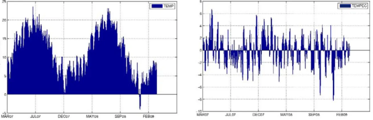
To take into account weather influences, we use the Tendances Carbone European

temperatures index, which is an average of national temperatures indices of four European

countries (France, Germany, Spain and the United Kingdom), weighted by the share of each National Allocation Plan. From this index, we have created three new variables:

tempec represents the difference between the value of the temperatures index and the

decennial average; temphot is a dummy variable for extremely hot temperatures (equal to 1 if the value of the temperatures index is higher than the third quartile of the series, and 0 otherwise); and tempcold is a dummy variable for extremely cold temperatures (equal to 1 if the value of the temperatures index is lower than the first quartile of the series; and 0 otherwise). The temperatures index and its deviation from decennial average are shown in Figure 7.

Figure 7: European Temperatures Index and Deviation from Decennial Average from March 9, 2007 to March 31, 2009

Source: Mission Climat Caisse des Dépôts

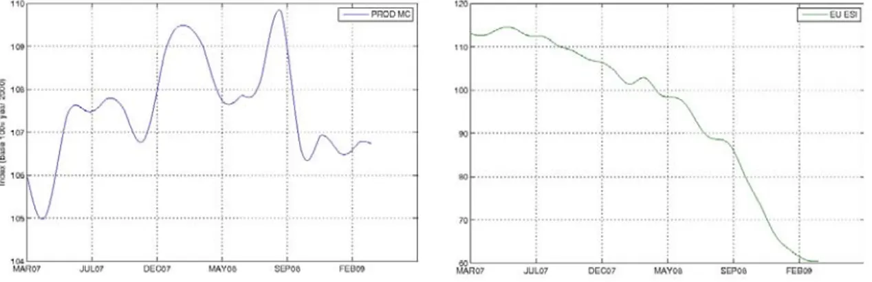
We have also introduced exogenous variables impacting CO2 emissions levels. First, we

consider the Tendances Carbone European Industrial Production index indicator, which uses Eurostat production indices and is a backward-looking indicator tracking past economic trends. Second, we use the Economic Sentiment Index published by Eurostat, which reflects overall perceptions and expectations at the individual sector level in a single aggregate index. This index is a forward-looking indicator used to mirror economic sectors’ sentiment. Finally, the “credit crunch” crisis may also have an impact on CO2 emissions

levels. To detect this potential influence, we have created the variable crisis as a dummy variable equal to 1 from August, 17 2007 onwards and 0 otherwise. This date corresponds to the first cut in interests rates by the U.S. Federal Reserve, and may be considered as the beginning of the financial crisis (Chevallier (2009)). Figure 8 shows the European Industrial Production Index and the European Sentiment Index variables.

Figure 8: Tendances Carbone Industrial Production Index (Weighted by the Share of NAPs) and EU Economic Sentiment Index

Source: Mission Climat - Caisse des Dépôts, Eurostat.

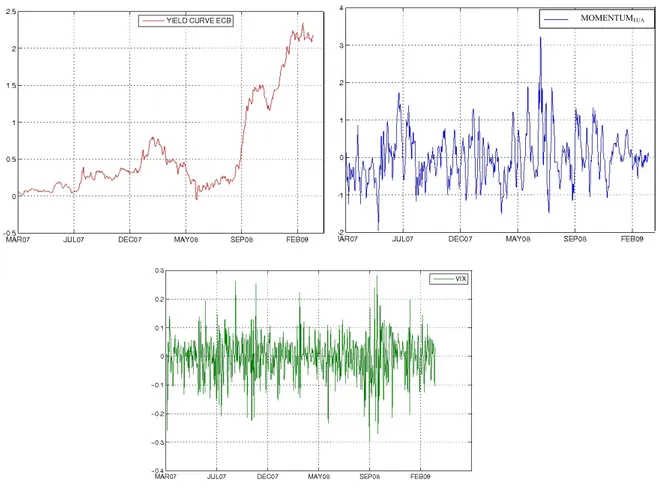
Additionally, we consider three other variables relevant to market trends. First, to take into account the slope of the Euro area yield curve, we have used the yield variable, which is available from the European Central Bank.17 _{This series is built as the spread between the}

5- and the 2-year interest rates. A positive (negative) value of the variable yield is expected to indicate an upward-sloping (downward-sloping) interest rate term structure, and hence a trend to cool down (stimulate) the economy (Collin-Dufresne et al. (2001)). Second, we have computed the momentumEUA variable. This variable represents the difference between

ECX EUA Phase II Futures prices at time t and at time t-5, thereby indicating bullish or bearish carbon market trends. Finally, VIX is the volatility index published by the Chicago Board Options Exchange (CBOE), which is widely recognized as an indicator of aggregate market volatility among financial practitioners (Collin-Dufresne et al. (2001)). Figure 9 presents the evolution of the three variables.18

17 _{Data can be found at : http://sdw.ecb.europa.eu}

18 _{Note we leave for further research the investigation of other potential explanatory variables, such as EUA} forward curves and the return on investment for EUAs growing at the EURIBOR rate.

Figure 9: Slope of Yield Curve, Market Momentum, and VIX Index from March 9, 2007 to March 31, 2009

MOMENTUMEUA

Source: European Central Bank, Reuters and CBOE

Regarding news variables that may impact the supply of EUAs, we consider three types of events. First we take into account the arrival of new information concerning Phase II

NAPs. Second, we consider news related to the extended development of the EU ETS

during Phase III. These two dummy variables have been constructed by filtering the most reliable and significant announcements on EU ETS developments from the European Commission website.19 _{Third, we also take into account the likely impact on EUA prices}

provoked by the connection between the Kyoto Protocol’s International Transaction Log (ITL) and the EU ETS’ Community Independent Transaction Log (CITL) on October 10, 2008 throughout the ITL-CITL dummy variable. This variable takes the value of 1 when news concerning the connection occurred and 0 otherwise.

After transforming, when necessary, the exogenous variables of our database into stationary variables, we detail in the next section the GARCH modelling for the EUA variable.

4.2. GARCH Modeling

We model the EUA variable by using the asymmetric TGARCH (p,q) model by Zakoian (1994) with a Student’s t innovation distribution, estimated by Quasi Maximum Likelihood with the BHHH algorithm:

t t t t t t t EUA t t t t t t t t t t t CITL ITL NAPphaseII III EUETSphase VIX crisis momentum yield EUESI MCprod tempcold temphot tempec switch gas coal brent EUA ε ν θ μ ϑ λ κ ι ϖ η γ ϕ φ ξ δ χ ρ α + + + + + + + + + + + + + + + + + = _

( )

( )

( )

with EUAt the residuals of the VAR(4) model related to the EUA at time t, α the

constant, brentt, coalt, and gast are the returns of the brent, coal and gas series, switcht the

switch variable, tempect, temphott, tempcoldt the temperatures variables, MCprodt the

industrial production index from Tendances Carbone, EUESIt the EU Economic Sentiment

Index, yieldt the slope of the Euro area yield curve, momentumEUAt the momentum variable

concerning the EUA market, crisist the dummy variable accounting for the “credit crunch”,

VIXt the CBOE volatility indicator, EUETSphaseIIIt the dummy variable for Phase III news,

NAPphaseIIt the dummy variable for Phase II news, ITL_CITLt the dummy variable for the

ITL-CITL connection, εt the error term, σt the conditional volatility, the subscript index t

refers to date t.

( )

( )

Lε are the positive and negative errors of the mean equation lagged one period respectively, and

( )

Note that in this model

( )

t

Lε and

( )

t

Lε capture asymmetric effects.

4.3. Estimation results

By estimating the TGARCH model presented in Section 3.2 and removing one by one non-significant exogenous variables, we are able to identify two different sets of regression results. In Table 4, regression (1) includes the main energy variables, while regression (2) contains the switch and other market variables. The quality of the regressions is verified following several diagnostic tests: the Adjusted R2_{, the Log-Likelihood ratio, the ARCH}

Lagrange Multiplier (LM) test, the Ljung-Box Q-test statistic with a maximum number of lags of 20 (Q(20) statistic), the Akaike Information Criterion (AIC) and the Schwartz Criterion (SC). For both models, the Ljung-Box-Pierce test indicates that residuals are not autocorrelated, and the Engle ARCH test indicates that heteroskedasticity is adequately captured by the structure of the TGARCH model. Besides, we have investigated the presence of multicolinearity by computing the matrix of partial cross-correlations and the

inflation of variance between explanatory variables.20 _{These calculations did not reveal}

serious problematic multicolinearities.

Table 4: TGARCH (1,1) Regression Results for the EUA Price Drivers

Variable EUAt (1) (2) Constant 0.0008 (0.0008) 0.0011 (0.0008) Brentt 0.0013*** (0.0003) Coalt -0.0017*** (0.0003) Gast 0.0003*** (0.0001) Switcht 0.0006*** (0.0002) MomentumEUAt 0.0082*** (0.0007) 0.0083*** (0.0007) NAP phase IIt -0.0084* (0.0044) -0.0095* (0.0049) Adjusted R2 _{0.1916 0.1631} Log-Likelihood 1287.749 1274.906 ARCH LM Test 0.7950 0.6360 Q(20) Statistic 26.789 24.322 AIC -4.7811 -4.8243 SC -4.9667 -4.7673 N 529 529

Note: EUAt refers to the residuals of the VAR(4) model related to the EUA (ECX EUA Phase II Futures). ***,(**),(*) Denotes 1%,(5%),(10%) significance levels. The quality of regressions is verified through the following diagnostic tests: the adjusted R-squared (Adjusted-R2_{), the Log-Likelihood, the ARCH Lagrange Multiplier (ARCH} LM Test), the Ljung Box Q-test statistic with a maximum number of lags of 20 (Q(20) statistic), the Akaike Information Criterion (AIC), and the Schwarz Criterion (SC). The 1% (5%) critical value for the Ljung-Box portmanteau test for serial correlation in the squared residuals with 20 lags is 37.57 (31.41). N is the number of observations.

In regression (1), we observe that energy variables have an impact on the EUA variable at statistically significant levels, which is conform to previous literature (Mansanet-Bataller et al. (2007), Alberola et al. (2008)).21 _{Brent and gas have a positive impact on EUA price}

changes: increases in fuel prices are directly transmitted to the CO2 allowance market. As

the most CO2-intensive fuel, coal has a negative impact on CO2 prices. This implies that

when the coal price increases, industrials have an incentive to use less CO2-intensive fuels,

which decreases the demand and the price of CO2 allowances. In regression (2), we uncover

the influence of two other variables: momentumEUA is positive and statistically significant at

the 1% level, while the dummy variable NAP Phase II is negative and statistically significant at the 10% level. The sign of the latter variable is conform to our expectations:

NAPs II allocations were reduced by 10% compared to NAPs I. This stricter constraint did not impact positively EUAs due to the context of the economic crisis, which was reflected primarily in the decrease of production outputs (and as consequence in reduced CO2

emissions from EU ETS installations). The positive sign of momentumEUA may be explained

by the fact that EUA price changes responded positively to carbon market trends during our study period.

In regression (2), we uncover the explanatory power of the switch variable at the 1% level. Its positive sign confirms that when the coal price increases, it becomes more profitable for power operators to switch from coal to natural gas including CO2 costs. Both

the momentumEUA and NAP Phase II variables are also significant with similar coefficients

and signs as in regression (1), which confirms the robustness of our previous estimates. Having reviewed the main price drivers of the EUA variable, we extend in the next section our investigation to the fundamentals of sCERs.

5. sCER Price Drivers

We focus in this section on the modeling of the sCER variable defined as the residuals of the VAR(4) model for the sCERs.22 _{To our best knowledge, this constitutes the first}

empirical analysis of sCER price drivers.

5.1. Exogenous variables

As for EUAs, it is important to distinguish between demand and supply factors affecting sCERs. Contrary to the allocation of EUA, the supply of sCERs is unknown. The main sources of uncertainty are due to the fact that (i) the supply of primary CERs is unknown and difficult to estimate (as it depends on several risks related to the issuance of primary CERs); and (ii) the amount of primary CERs that will be converted into sCERs is also difficult to assess (see Trotignon and Leguet (2009). On the demand side, whereas on the EU ETS the demand comes from private financial or industrial operators, for sCERs the demand comes from a larger number of participants (investors, industrials and Annex-B countries). Most of the CERs demand to date comes from European industrials, which are limited to 13.4% (on average) of surrendered allowances for compliance during Phase II of the EU ETS. Besides, Annex-B countries of the Kyoto Protocol may also use CERs for compliance. Countries with a potential deficit of Assigned Amount Units (AAUs valid under the Kyoto Protocol) in 2012 - such as Japan - are involved in sCERs purchasing. Among other factors that may impact sCERs prices, we identify the same factors as those affecting EUAs prices, since both assets may be used for compliance in the EU ETS.

22 _{Note that as the drivers of primary and secondary CER are not the same, it is important to remind here that} we are considering secondary CER prices.

Hence, we consider the same explanatory variables as for EUAs in sCERs pricing. That is, energy prices (brent, gas and coal), the switch price variable, temperatures variables, variables related to production levels, market volatility, and dummy variables related to the announcements concerning the status of the CDM in Phase III of the EU ETS and the ITL-CITL connection. Note that we have computed a new specific variable, called

momentumsCER, for the indication of bullish and bearish periods. Similarly to the case of the

momentumEUA variable, the momentumsCER variable is obtained as the difference between

the sCER variable at time t and at time t-5.

Besides, we add three variables that take into account the specificities of sCERs (mostly related to the supply side): (i) CDM EB meeting, (ii) linking, and (iii) CDMpipeline.

The dummy variable CDM EB meeting is equal to 1 on the publication date of CDM EB’s reports, and 0 otherwise. This variable indicates the arrival of new information from the United Nations’CDM Executive Board. The dummy variable linking is equal to 1 when there on the announcement date related to the linking of emissions trading schemes worldwide, and 0 otherwise.23

Finally, the CDMpipeline variable is the forecast error concerning the number of primary CERs actually delivered by the CDM EB. Each month, the UNEP Risoe announces how many primary CERs are expected to be delivered in the CDM Pipeline.24 _{This variable}

is computed following the approach developed by Kilian and Vega (2008):

σ

With Realisedt the announced value of the amount of primary CERs delivered by the

UNEP Risoe, Expectedt the market’s expectation of the amount of primary CERs to be

delivered prior to the announcement, calculated by Trotignon and Leguet (2009), and

σ

Figure 10: Forecast errors for the number of CERs available in the CDM Pipeline from May 2008 to March 2009

Source: UNEP Risoe and Mission Climat Caisse des Dépôts

5.2. GARCH modeling

We model sCER prices by following the same methodology as for EUA Phase II Futures prices: t linking ng CDMEBmeeti e CDMpipelin t CITL ITL t III EUETSphase t VIX t crisis sCERt momentum t yield t EUESI t MCprod t tempcold t temphot t tempec t switch t gas t coal t brent t sCER t t t ε υ ς π ν μ ϑ λ κ ι ϖ η γ ϕ φ ξ δ χ ρ α + + + + + + + + + + + + + + + + + + + = _

( )

( )

( )

with sCERt are the residuals of the VAR(4) model related to the sCERs at time t,

momentumsCERt, CDMpipelinet, CDMEBmeetingt, and linkingt exogenous variables specific

to sCERs defined as above. Other variables have been defined previously for the EUA variable.

5.3. Estimation results

Estimation results are presented in Table 5. The quality of the regressions (3) to (5) is verified with the same diagnostic tests as for EUAs. All diagnostic tests are validated for regressions (3) to (5).

In regression (3), we observe that energy prices (brent, coal lagged one period, and gas) have a statistically significant impact on sCER prices with the same signs as for EUAs. This first result confirms that EUAs and sCERs share basically the same price fundamentals with respect to the interaction with energy markets.

In regression (4), momentumsCERt and linking are statistically significant at the 1% and

10% levels, respectively. The sign and interpretation of momentumsCERt is similar to

momentumEUAt in the case of the EUA variable.

The positive sign of linking suggests that news about the future connection between the European and international credits carbon markets tend to increase sCERs prices. Note that sCERs are fungible across regional and domestic markets. Thus, this positive sign is coherent with what we would expect: as the global demand of sCERs increases, the price of sCERs also increases.

In regression (5), we note that CDMpipeline is not significant in explaining sCERs price changes. This result is conforming to the view that sCERs have distinct fundamentals from the delivery of primary CERs, since they are free of project delivery risk.

Table 5: TGARCH (1,1) Regression Results for the sCER Price Drivers

Variable sCERt (3) (4) (5) Constant _0.0008 (0.007) 0.0007 (0.0007) 0.0007 (0.0013) brentt 0.0009*** (0.0002) 0.0005* (0.0003) coalt-1 0.0008** (0.0001) -0.0017*** (0.0003) gast 0.0002*** (0.0001) 0.0002* (0.0001) momentumCERt 0.0093** (0.0009) 0.0098*** (0.0009) Linkingt 0.0194* (0.0111) CDM pipelinet 0.0005 (0.0013) Adjusted R2 _{0.1582 0.1427 0.0469} Log-Likelihood 1344.581 1339.208 660.743 ARCH LM Test 0.9195 0.9730 0.7560 Q(20) Statistic 25.137 24.396 20.724 AIC -5.1074 -4.8026 -4.5827 SC -5.0341 -4.7783 -4.4542 N 529 529 529

Note: sCERt refers to the residuals of the VAR(4) model related to sCERs (Reuters sCER Price Index). ***,(**),(*) Denotes 1%,(5%),(10%) significance levels. The quality of regressions is verified through the following diagnostic tests: the adjusted R-squared (Adjusted-R2_{), the Log-Likelihood, the ARCH Lagrange Multiplier (ARCH} LM Test), the Ljung Box Q-test statistic with a maximum number of lags of 20 (Q(20) statistic), the Akaike Information Criterion (AIC), and the Schwarz Criterion (SC). The 1% (5%) critical value for the Ljung-Box portmanteau test for serial correlation in the squared residuals with 20 lags is 37.57 (31.41). N is the number of observations.

Having detailed separately EUAs and sCERs price drivers, we now turn to the determinants of the price difference between these two emissions assets.

6. EUA-sCER Spread drivers

Following the analysis of EUAs and sCER price drivers, we focus in this section on the variables that may have an explanatory power for the evolution of the EUA-sCER spread defined as follows:

t t

t EUA sCER

Spread = −

With EUAt and sCERt respectively, the EUA (ECX EUA Phase II Futures prices) and

sCER (Reuters sCER Price Index) rolled-over futures contract prices.25 _{The EUA-sCER}

spread is pictured at the bottom of Figure 1. Given its construction, the spread is positive. It is equal to €2 in March 2007, €8 in May 2007, and evolves in the range of €2 to €6 until May 2008. It becomes then relatively close to zero until March 2009. Thus, the spread seems to widen (narrow) depending on bullish (bearish) periods on emissions markets. In Figure 11, we observe that the EUA-sCER spread taken in stationary first-difference transformation exhibits volatility clustering from May to September 2008, and that the volatility decreases near the end of the sample period.

Figure 11: First-difference of the EUA-sCER Spread from March 9, 2007 to March 31, 2009 -2.0 -1.5 -1.0 -0.5 0.0 0.5 1.0 1.5 100 200 300 400 500 FIRST_DIFF_SPREAD

25 _{Note that ECX has implemented a sCER-EUA trading facility that allows trading the spread at reduced} transaction costs. To facilitate the understanding of the determinants of the spread, we have chosen the more intuitive definition of the Spread = EUA-sCER, which has the advantage to be positive over the sample period.

The EUA-sCERs spread trading is mostly used by industrial and financial operators involved in short term trading activity. Indeed, the supply and demand for EUA-sCERs spread contracts come from short term price differences between EUAs and sCERs (as shown in Figure1). At time t, it appears profitable for investors to swap between these two carbon assets by buying sCERs and selling EUAs, since both assets may be used for compliance in the EU ETS (as long as the import limit on CERs is not reached). However, not all market participants may benefit from this arbitrage strategy. The reason for that situation is twofold: (i) there exist different types of market participants with different kinds of obligations and flexibility requirements on the use of sCERs, and (ii) technical skills are required to simultaneously buy sCERs and sell EUAs.

The latter point means that while banks may trade EUAs and sCERs on the market, they cannot use them towards their own compliance (and thus benefit from the full scale of the arbitrage strategy), since they are not regulated by the scheme. Conversely, large regulated utilities such as energy trading companies may benefit from opening a carbon trading desk in-house and exchange sCERs for EUAs in their own registry account. This type of market participant is therefore able to arbitrate between the two emissions markets by buying sCERs on the market and selling EUAs (registering them in its own registry towards compliance with their emissions target) when the price difference between the two emissions markets is at its maximum. This strategy yields a net “free-lunch” benefit as long as the import limit on CERs is not reached (which is not likely to be reached anytime soon according to the analysis by Trotignon and Leguet (2009)).

6.1. Exogenous variables

Besides the variables that have been previously identified as impacting EUAs and sCERs, we use price thresholds, market activity and liquidity variables stemming from the market microstructure literature (Codogno et al. (2003), Manganelli and Wolswijk (2009)) that may have an explanatory power for the EUA-sCER spread.

Regarding price thresholds, EUApricelevel is computed by regressing the EUA-sCER spread against the time-series of EUA prices. This variable reflects the idea that investors would more easily trade the spread if EUAs prices are around €30 than if they drop to €5. Following Zhang (2002), we also use a threshold variable (noted thresholdSpread) defined at €6 for the EUA-sCER spread.26 _{Above this threshold, investors are expected to}

simultaneously sell EUAs and buy sCERs. Below, they are expected to wait for the widening of the spread to benefit from future more profitable arbitrage opportunities. Note

that this behavior is coherent with the fact that the import of CERs in the EU ETS (and thus the arbitrage opportunity) is limited in quantity and through time.

Regarding market activity, we use the average trade size for ECX EUA Phase II Futures prices (averagetradeEUA), defined as the daily volume divided by the daily number of trades, in order to track the impact of block trades or quasi-block trades on the spread. One could expect that large primary CER issuance could translate into large movements in the EUA market for cashing on the spread. Additionally, we have defined the variable

openintEUA as the level of the open interest for the prevailing EUA calendar futures

contract. This variable reflects the market overall level of engagement with the underlying asset. Compared to cumulative volumes, the open interest measure has the advantage to neutralize the impact of further transactions on existing futures positions to other market participants. The larger the open interest, the larger the quantity of futures contracts to be settled at a given date. We have also created the variable CDMmktdvlpt as a dummy variable equal to 1 during news announcements regarding the ability to trade sCERs (such as the beginning of trading sCER throughout standardized contracts on market places, etc.) and 0 otherwise.27 _{We expect more activity on the spread as more announcements are}

recorded. Moreover, numbertradeEUA indicates the daily number of trades performed on ECX EUA Phase II future prices, as a proxy for liquidity in the market. This variable also reflects market participants’ increased technical skills, as they may resort to specific algorithms to “slice up” large orders. Figure 12 displays the openintEUA,

numbertradeEUA, and averagetradeEUA variables.

Figure 12: ECX EUA Futures Open Interest (left), BNX Daily Number of Trades (right), and Average value of Orders (below) from March 9, 2007 to March 31, 2009

Source: ECX and Bluenext

To detect whether the size of the EUA-sCER spread is affected by changes in market activity and more specifically by market liquidity, we have considered trade-based measures for EUAs and sCERs. More precisely, following Gómez-Puig (2006), we have instrumented the ΔvolumeEUA variable, which tracks changes in the volume of EUAs traded, and the ΔvolumesCER variable, which tracks changes in sCERs volumes exchanged.28 _{Figure 13 shows the evolution of these two variables.}

Figure 13: ECX EUA Futures (left) and Reuters CER Index (right) Volumes from March 9, 2007 to March 31, 2009

Source: ECX and LEBA

By using the (intraday) order book for EUAs, we computed relative bid-ask measures for EUAs (bidaskEUA). We systematically checked relative bid-ask spreads over 10% and below 1% (i.e. out of the established trend), and manually removed outliers that most likely reflected market orders made without any chance of being fulfilled.29 _{Hence, the “cleaned”}

bid-ask used is a proxy for real liquidity of EUAs. We applied the same methodology with brokers’ bid-ask data from the Reuters CER index (bidasksCER). The index contains daily average bid and ask prices from eight representative carbon brokers, so that no recalculation was required to proxy market liquidity on a daily basis. Figure 14 shows the

bidaskEUA and bidasksCER variables.

Figure 14: Bid-ask spread for ECX EUA Futures (left) and Reuters CER Index (right) from March 9, 2007 to March 31, 2009

Source: ECX and Reuters

29 _{Bid-ask spreads may be negative according to our calculations since: (1) we are interested in daily average} bid and ask, hence smoothing any intraday move; and (2) some bids or asks could have been posted with no intent of being attractive, but rather by contractual obligations (for market makers), or to deceive. Those bids and asks distort our estimation of bid-ask spreads. There is no economic rationale behind a negative bid-ask for a single quote, but it could indicate strong intraday activity.

Finally, we use Panic as a dummy variable equal to 1 from October 10 to 17, 2008; and 0 otherwise. This variable reflects the sharp increase in the volatility of EUA prices that may be observed in October 2008, as regulated utilities were “rushing to cash” in search for liquidity, in order to cope with the credit crunch crisis according to market observers.30

6.2. GARCH modeling

We model the EUA-sCER spread by following the same methodology as for the determinants of EUA and sCER variables:

t t t t t t t t t t t t t t t t t t t t EUA t pread thresholdS bidasksCER bidaskEUA volumesCER volumeEUA deEUA averagetra vel EUApricele EUA open eEUA numbertrad t CDMmktdvlp linking ng CDMEBmeeti panic CITL ITL III EUETSphase crisis e CDMpipelin VIX momentum Spread ε γ ς ϖ β ξ η χ ψ φ ω ν ς ν μ λ π υ κ α + + + + Δ + Δ + Δ + + + + + + + Π + + + + + + + = int _

( )

( )

( )

with Spreadt the first-differenced EUA-sCER spread, CDMmktdvlptt,

numbertradeEUAt, openintEUAt, EUApricelevelt, averagetradeEUAt, volumeEUAt,

volumesCERt, bidaskEUAt, bidasksCERt, thresholdSpreadt are the exogenous variables

specific to the EUA-sCER spread commented above. Other variables have been defined previously for the analysis of EUA and sCER price drivers. Exogenous variables have been transformed to stationary when needed.

6.3. Estimation results

Table 6 presents the estimation results for the EUA-sCER spread. All diagnostic tests are validated for regressions (6) and (7).

Note that a statistically significant positive (negative) coefficient means that the spread is widening (narrowing) following changes in the underlying explanatory variable.

Table 6: TGARCH(1,1) Regression Results for the EUA-sCER Spread Drivers

Variable Spreadt

(6) Spread(7) t

Constant 0.0145

(0.0111) (0.0134) -0.0080

EUA price levelt -0.9562***

(0.0322) -0.6726*** (0.0469) Δ volume EUAt 0.0007** (0.0004) 0.0001*** (0.0001) Δ volume sCERt 0.0013** (0.0007) MomentumEUAt -0.0945*** (0.0121) -0.0997*** (0.0151) Linkingt 0.2610*** (0.0733) VIXt 0.3364*** (0.1213) Crisist -0.4299*** (0.0711) CDM EB meetingt -0.0901*** (0.0541) ThresholdSpreadt 0.0764*** (0.0134) CDM pipelinet -0.0161*** (0.0013)

Open interest EUAt 0.0001***

(0.0001) Adjusted R2 _{0.5800 0.5658} Log-Likelihood 141.5910 79.0179 ARCH LM Test 0.5540 0.5278 Q(20) statistic 36.765 26.371 AIC -0.5023 -0.4699 SC -0.4209 -0.3016 N 529 529

Note: Spreadt = EUAt-sCERt. EUA refers to ECX EUA Phase II Futures prices. sCERt refers to Reuters sCER Price Index. ***,(**),(*) Denotes 1%,(5%),(10%) significance levels. The quality of regressions is verified through the following diagnostic tests: the adjusted R-squared (Adjusted-R2_{), the Log-Likelihood, the ARCH Lagrange} Multiplier (ARCH LM Test), the Ljung Box Q-test statistic with a maximum number of lags of 20 (Q(20) statistic), the Akaike Information Criterion (AIC), and the Schwarz Criterion (SC). The 1% (5%) critical value for the Ljung-Box portmanteau test for serial correlation in the squared residuals with 20 lags is 37.57 (31.41). N is the number of observations.

In regression (6) we observe that the EUApricelevelt variable has a strong and

statistically significant explanatory power for the determination of the EUA-sCER spread. As highlighted previously, sCER and EUA prices have followed similar price paths over the period. Thus, changes in EUA prices have a strong effect on the EUA-sCER spread. The sign of the EUApricelevelt coefficient is negative, which suggests that when EUA

prices increase, the EUA-sCER spread diminishes. This result supports the intuition that at higher EUA price levels, investors and market operators have higher incentives to take adequate positions in both emissions markets to take advantage of the EUA-sCER spread. On the contrary, at low levels of EUA prices, the EUA-sCER is narrowing, which yields less profitable arbitrage opportunities. Interestingly, the coefficients of the ΔvoumelEUAt

and ΔvoumelsCERt variables are statistically significant and positive. This result indicates

that increased trading of EUAs and sCERs translates into wider EUA-sCER spread. This view is conform to the use of the EUA-sCER spread as a speculative product by rational

investors and arbitrageurs: the volumes exchanged for EUAs and sCERs are found to be the highest when the EUA-sCER spread is at its maximum – thereby reflecting the strategy to maximize net profits.

The momentumEUAt and linkingt variables have a statistically significant impact on

variation of the EUA-sCER spread. The sign of momentumEUAt is positive, which suggests

that when this variable is increasing (on a bullish carbon market), the EUA-sCER spread is narrowing. This result illustrates in a similar way the profit-maximizing strategy of rational market participants in the carbon market through the use of the EUA-sCER spread. Conversely, on a bearish carbon market (indicated by decreases in the momentumEUAt

variable), the EUA-sCER spread is widening, which provides future opportunities for market participants to make the spread transaction at better conditions.

As indicated by the positive coefficient of the linking variable at the 1% level, the development of an international carbon market accepting sCERs as compliance assets tends to widen the EUA-sCER spread. Indeed, the prospects for growing sCERs demand outside of the European trading system might lead to a partial decorrelation from EUAs in a near future.

News regarding Phase III of the EU ETS, the ITL-CITL connection and market liquidity (as proxied by bid-ask spreads) could not be identified as statistically significant variables in regression (6).

Regression (7) is similar to regression (6), and reveals the explanatory power of six additional variables. The EUApricelevelt, the ΔvolumesEUAt, and the momentumEUAt,

coefficients may be interpreted identically. Changes in the VIX index, which are obtained from the implied volatility of S&P option prices, are used as a proxy of the evolution of aggregate financial markets’ volatility. Its positive and statistically significant coefficient indicates that the EUA-sCER spread widens when the stock market volatility increases. This increase in the spread may indicate that the risk of holding sCER is perceived as higher than holding EUAs, which translates into a higher risk premium for the sCERs.

The crisis dummy variable appears statistically significant with a negative coefficient. Since the start of the global financial crisis, the EUA-sCER spread has narrowed, which suggests a strong interest in selling EUAs. Two facts may help to understand this negative coefficient. First, the global financial downturn has caused a decrease in industrial production and energy demand (and thus in the energy production of CO2-intensive plants).

The need for CO2 allowances has dropped drastically, which fostered incentives to sell

EUAs and contributed to the decline of the EUA-sCER spread. Second, as a consequence of the crisis, funding needs have increased. From this perspective, selling EUAs (which are only needed for compliance on April 30th _{of the year N+1) constitutes a sound strategy in}