Eddy dynamics of [Beta] plumes

Eddy dynamics of

#3

plumes

by

Shinichiro Kida

B.Sc. in Earth and Planetary Physics The University of Tokyo, 2000

Submitted in partial fulfillment of the requirements for the degree of Master of Science

at the

MASSACHUSETTS INSTITUTE OF TECHNOLOGY

and the

WOODS HOLE OCEANOGRAPHIC INSTITUTION September 2003

@ Shinichiro Kida, MMIII. All rights reserved.

The author hereby grants to MIT and WHOI permission to reproduce and distribute publicly paper and electronic copies of this thesis document in whole or in part.

A uthor ... . . .. ... ...

Joint Program in Oceanography/Applied Ocean Science and Engineering Massachusetts Institute of Technology Woods Hole Oceanographic Institution K-ntember, 2003 C ertified by ... .. ... ... C ertified by ... Accepted by ... ... Jiayan Yang Associate Scientist - Tfesis Supervisor James F. Price Senior Scientist Thesis Supervisor .... ... Carl Wunsch Chairman, Joint Committee for Physical Oceanography Massachusetts Institute of Technology Woods Hole Oceanographic Institution

Eddy dynamics of

#

plumes

by

Shinichiro Kida

Submitted to the Massachusetts Institute of Technology and the Woods Hole Oceanographic Institution in partial fulfillment of the requirements for the degree of

Master of Science

Abstract

The importance of eddies and nonlinearities in

#-plume

dynamics in the deep ocean was investigated using reduced gravity models of the deep ocean forced by a small

region of cross isopycnal transport in the interior. The effect of topography on 0-plimes was also examined by placing a Gaussian bump in the forcing region. Despite the fact that the mean flow is weak in the deep ocean interior, it was found that the nonlinearity and instabilities are still important for realistic parameter and forcing values. The flow was dominated by eddies and was remarkably different fromi what would be expected from a linear solution.

Thesis Supervisor: Jiayan Yang Title: Associate Scientist

Thesis Supervisor: James F. Price

Acknowledgments

I would like to thank my advisers, Dr. Jiayan Yang and Dr. Jim Price for spending enormous amount of time for discussion and guidance. I can not thank them enough

for the advice and feedback they provided me. In addition to the weekly discussions,

their constant warn support inade it possible for ime to enjoy my research and also

the field of Physical Oceanography. I would also like to thank Dr. Karl Helfrich for guiding ine through much of the literature on hydrothermal plumes. The research

on this topic would not have gone as smoothly without his help. My thanks also goes to Dr. Joe Pedlosky for thorough answers to many of my questions, Prof.

John Marshall for the providing me the computer resources at MIT, and my thesis

committee members, Drs. Robert Beardseley, Glenn Flierl, and Carl Wunsch for their valuable comments that improved nany parts of this study.

I feel very fortunate to have such wonderful classmates, J. Ton Farrar, Jason Hyatt and Mitch Ohiwa. Their encouragement through the years meant a lot to ine. The discussions with Geoffrey Gebbie, Baylor Fox-Kenper, and Taka Ito also improved my research. Thanks also to miy officemnates, Juan Botella, Juli Atherton, Fabio Dalan,

David Stuebe, and Max Nikourachine for making miy life at MIT comfortable. Last, I would like to thank my parents, Hideji and Yasuko Kida. Their love and

support from Japan made it possible for ine to enjoy imy studies here in the United States.

This study was supported by Woods Hole Oceanographic Institution Academic

Contents

1 Introduction ₉

1.1 What is a 0-pluie?... . . . . . . ... 9

1.2 Single Hydrothermal Pliiie Events... . . . . . . . . . 15

1.3 Topography. ... . . . . . . ... 16

1.4 Present work . . . . 17

2 Model Description and Basic theory 21 2.1 Numerical Model... . . . . . . 21

2.2 _{B asic theory . . . . 29}

3 Numerical Model Result: The effect of Nonlinearity in a flat bottom basin ₃₅ 3.1 Barotropic 1-phime: Case 1... . . . . . . . . ... 35

3.2 Baroclinic /3-plimile: Case 2... . . . . . .. . 41

4 The effect of bottom topography ₅₅ 4.1 Linear Solution... . . . . ... 55

4.2 Barotropic /3-plume: Case 3... . . . . . . . 60

4.3 _{Baroclinic O-pluie: Case 4 .. . . . . . . . 66}

5 Summary and Conclusion ₇₅ 5.1 Summary... ... .. ... .. .... . . . ... 75

Chapter 1

Introduction

1.1

What is a /-plume?

A 3-pluie is a large scale horizontal circulation driven by a localized mass source or sink. It was introduced b y Stommel (Stormmel 1982) who was inspired by an observational result which show an anomaly of helimn from the hydrothermal vents extending to the west of East Pacific Rise (Lupton 1984). This feature was unexpected

at the time, for the circulation at this location (900 - 1341W, 15'S) was believed to be a weak southeast flow according to the Stommel and Arons Model (Stormcl and

Arons 1960). Stonnel then showed that a, hydrothermal vent is capable of driving a

large horizontal circulation on its own by using a linear vorticity balance equation;

fow*

#3v H (1.1)

H

where

f

0,

#3,

v, w*, and H are the Coriolis parameter, its meridional gradient, mnerid-ional velocity, cross isopycnal velocity, and layer thickness respectively. More detailed

description of this equation and terns will be given later. This linear vorticity

equa-tion (Eq 1.1) is a balance between planetary vorticity advecequa-tion (LHS) and vortex

stretching(w* > 0) or squashing(w* < 0) (RHS). For a wind driven gyre where this linear vorticity balance is known as Sverdrup balance, Ekmnan pumping causes vortex stretching/squashing and drives a meridional flow. For a

#-plume,

the cross isopycnal

transport created by the hydrothermal vents causes vortex stretching/squashing and drives a Ineridional flow. However, the ineridional flow can establish only in limited areas because unlike wind forcing, hydrothermlal vents do not exist all over the basin. Figure 1-1 shows the basic concept schematically. Through geothermal heating, the water near the vent is heated and rises to its neutrally buoyant layer as it entrains the surrounding water. For the neutrally buoyant layer, this cross isopycnal trans-port leads to vortex squashing. From Eq 1.1, vortex squashing creates a southward flow. In order to balance this southward flow, there needs to be a northward flow somewhere in the basin. Since there can not be any ineridional flow in the interior where hydrothermal vents do not exist, an anticyclonic circulation consisting of a northward western boundary flow, a westward zonal jet and an eastward zonal will establish. For the layer below the neutrally buoyant level, the opposite mechianism causes vortex stretching and a cyclonic circulation will establish. Figure 1-2 is the steady solution for each layer. A linear two-and-a-half layer reduced gravity model described in the next chapter was used to calculate this steady solution. These two counter rotating circulations are what has been called the "#-plumne." The concept of 0-phlmes provided a nechanism for creating a strong zonal flow in the deep ocean.

A small cross isopycnal transport is capable of forcing a horizontal circulation of much larger order of magnitude than itself. For example, at 30'N, the linear vorticity balance (Eq 1.1) shows that a cross isopycnal transport of 0.01 Sv over an area 100kn(imeridional) x 100kmn(zonal) is capable of creating a horizontal transport of 3.5 Sv. The ratio of total cross isopycial transport(W) to horizontal transport(M) depends on a parameter f/#L which is a function of the latitude and meridional

length scale L of where the cross isopycnal transport exists. [Pedlosky 1996, Spall 2000. Suppose a region of constant cross isopycnal velocity (forcing region) exists in the interior as shown in Figure 1-3a. From linear vorticity balance, the total

neridional transport(M) across this forcing region is,

z0 y

_{N Equator}

x

isopycnal

w

vents

Ridge

Figure 1-1: Schematic Picture of a

#-plume

adapted from Stommel(1982). The upper

layer represents the neutrally buoyant density layer and the bottom layer represents

the layer below. The left boundary represents the western boundary. The water

heated by the vent entrains the surrounding water from the bottom layer and enters

the upper layer with a total cross isopycnal transport of W*. As a result of this cross

isopycnal transport, a cyclonic circulation is established in the bottom layer and an

anticyclonic circulation is established in the upper layer.

(a) Neutrally buoyant layer 400km- --- - - - - -- --- - -- -

--200 ----

-0400 800km

(b) Layer below the neutrally buoyant level

400km- --- - -

---200-

---

~---0 400 800km

Figure 1-2: Velocity field in the (a) Neutrally buoyant layer and (b) Layer below are

shown. The black circles indicates the forcing region. Velocity larger than 0.01 rn/s

are truncated and are shown in red. Only the values at every 5 grid points are shown.

For scaling, 0.01 rn/s is shown in the bottom right corner

(a) shows an anticyclonic circulation and (b) shows a cyclonic circulation. Meridional

flow exists only in the forcing region and the western boundary connected by the

two zonal

jets.

The weak zonal

jets

at the southern and northern boundary

(in both

figures) are created by the weak uniform background flow from the upper layer to

the layer below. It is a weak Stommnel and Arons type of circulation and thus is not

Forcing Region

(a)

m- - -m

(b)

Large Ly

weak flow

Strong flow Small Ly

Figure 1-3: A schematic of a

#-plume

when the water mass is leaving the layer: (a) The region of intense cross isopycial velocity (forcing region) is located in the interior of a rectangular basin. Assuming that the linear vorticity balance holds inside this forcing region, the total horizontal transport induced by the forcing is

Al = vL, = f* _O3HL. Using the total cross isopyenal transport (W = w*L.L,) across

the forcing region, The ratio shows that the induced horizontal transport

The total cross isopycnal transport in the forcing region is W = w*L LY so this equation (Eq 1.2) becomes

Ml

_{f Al}

____(1.3)

W ~3LYH

This parameter shows that the total meridional transport is inversely proportional to

the ineridional length scale of the forcing region.

Studies on

#-plumes

progressed by solving the stealy problem through theory, primarily because only a few observations were available in the deep ocean. It might

be argued that

#-plumes

are localized processes and thus might be insignificant in the presence of mean flows such as those in the Stormmel and Arons model, topographic effects

,

and wind forcing. Prior effort focused on this problen finds the 3-plume still significant enough in some region to compete with the mecan flow and to drive the deep circulation. Speer (1989) showed that the existence of a /-plume in the presence of a background Stommel and Arons flow depends on the ratio of long wave speed to the background flow which is large enough to overcome the background flow in some places. Hautala and Riser (19931) investigated a /-plume in the presence

of background Stonnel and Arons flow, topography, and wind forcing by solving a steady geostrophic three layer model. Their result also showed the strength of the

/3-plume to be significant enough to compete with other effects, at least locally. An

observational work of Hautala and Riser (1993a) which showed the effect of / plumes in the deep ocean, also seens to be in support of the previous theoretical studies.

The concept of

#-plumes

have been applied to regions besides deep ocean such as

the Mediterranean overflow. Localized entrainment of Atlantic Ocean water into the

overflow water is driving the /-plume in this case. Since w* is negative, the mechanism for this /3-plume works in the opposite sense creating a cyclonic gyre in the upper layer and an anticyclonic gyre in the lower layer since w* is negative. Jia (2000)

showed this nechanism to be a possible cause for the Azores current. Spal (2001)

and Ozgbkmen and Crisciani (2000) showed that friction is capable of diminishing or completely wiping out the

#-plume

when the forcing region (mass sink/source) is along the eastern boundary. The role of friction can not be neglected in

#-plume

dynaiics if the mass sink/source is close to the boundary.

There have been only a few studies on the effect of nonlinearities and instabilities on

#-plumes.

The results of Ozg5wkmn et al. (2001) shows the presence of barotropic instabilities in their calculations of the Mediterranean overflow case, although no detailed analysis of the role of these instabilities were given.

#-plumes

are also two layer events and baroclinicity can become important. How

#-plumes

are affected by nonlinearities and instabilities is an open question and will be a focus of this study.

1.2

Single Hydrothermal Plume Events

Single hydrothermal plune events have been studied theoretically (Speer 1989), nu1i-inerically (Speer and Marshall 1995), and through laboratory experiments (e.g.

Hel-frlich

and Battisti (1991)]. Most work concentrated on the formation and breaking

nechanismis of a single plume event. A hydrothermal phnie first rises to a level of neutral buoyancy and then starts to spread out laterally, forning a lenselike struc-ture. This lenselike structure creates an anticyclonic vortex in the neutrally buoyant density layer and a cyckmnic vortex below this layer. The lens structure is maintained

as the pluine increases laterally until it reaches the size of the deformation radius.

Then, the lens structure begins to break apart. The anticyclonic vortex in the neum-trally buoyant layer splits into an anticyclonic vortex and a cyclonic vortex and nany

vortices of different sign will eventually emerge in the region with each vortex having no particular preference on the direction in which it propagates (Hog and Stomriel

1985).

The evolution of a single plumie in the deep ocean is difficult to observe. Joyce et

al. (1998) showed two vortices of different sign on top of each other formed in one of

the mnega plume events in its early stages. D'Asaro et al. (1994) also found a vortex structure both in the young and mature mega plumes. Observations seem to support the formation nechanisn outlined above.

The studies of a single plumie event have been mainly based on a f-plane. This is because each plume event occurs on the order of a few kilometers and the change in

f

is negligible. The nonlinear nature of two vortices of different sign on top of each other have been well studied (e.g. Flicri (1988)) on the f-plane, but if a large scale effect of hydrothermal plumes were to be considered, 0 cannot be neglected from its dynamics. Nonlinear behavior of the large scale pluIme will be influenced by

#

which

could stabilize the vortex breaking observed in a

f

plane model. While there have

beeni many studies on nonlinear behavior of individual plume events in snall scales,

the nonlinear behavior of the large scale mean of many single plumes has not been well studied.

1.3

Topography

Hydrothernal vents typically lie on mid ocean ridges where topographic variations

are large compared to other parts of the ocean interior. Overflows also exist where

to-pographic variations are large. The regions where the concept of 3-plumnes are applied coincide to regions where topographic variation is considered large. The importance of topography on

#-plumes

has been addressed in some previous studies (Speer 1989), although its actual effect has not been studied adequately. The topographic

varia-tions can modify the background Potential Vorticity (PV) gradient, which will likely

change the basic circulation.

Kawase and Straub (1991) and Straub and Rhines (1990) investigated the (ffect

of topographic variation on the Stoiimmel and Arons Flow. Although their studies are based on the Stomnel and Arons flow, they showed an establishment of two zonal jets to the west of the topography similar to -plunes. This occurred when

the topographic variation was large enough to create a region of closed PV contour.

These two zonal jets existed roughly along the same latitude and were flowing in

the opposite direction. Uniforim mixing across the basin is capable of creating zonal jets in the presence of topography. However, further investigation is needed for cases when mixing is localized instead of uniform across the basin. The topographic effect of nonlinearity and instability will also need further investigation.

1.4

Present work

The motivation of this work is to examine the role of eddies and nonlinearities on the dynamics of

#-plumes.

As nentioned in the previous sections, past studies of large scale 0-plunes have focused more on linear dynamics while eddies were usually

neglected. However, this does not necessarily mean that the large scale plume has to be governed by linear dynamics. For example, can the narrow zonal jets really exist? Are they stable? Nonlinearities and instabilities could play an important role and influence the 0-plune.

Past studies of single hydrothermal plume events have focused on the formation and breaking nechanisin on a f-plane. The behavior of a large scale plumne, repre-senting series of single hydrothermal events with a large scale mean, will likely be influenced by

#

and behave differently from a single plume event. However, the non-linear dynamnics of single plume events turned out to be quite relevant to

#-plumres

found in this thesis. This thesis attempts to show that eddies and nonlinearities do influence the large scale

#-plume

with its dynamics somewhat similar to the

f

plane dynamics. It should be noted that the eddies that will be shown in this study are not the hydrothernal eddies created by some particular hydrothermal plume event or from interaction between hydrotherimal plumes. A large scale mean of the effect of many hydrothermal events was used because the resolution was not high enough to sufficiently resolve the dynamics of each hydrothernal plumne event.

Topographic effects will also be investigated. Not only can topography change the structure of the

#-plume

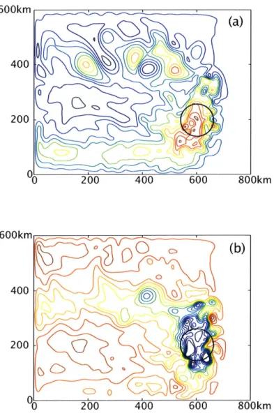
but it can also change the instability mechanism because of the topographic 3 effect. The importance of nonlinearities and instabilities can also change with the topographic variation.

Figure 1-4 is a result of the same reduced gravity model as the one used for Figure 1-2 but now with nonlinearity and varied bottomi topography. Compared to Figure 1-2 where the model was linear with a flat bottom, it is apparent that nonlinearity and varied topography do affect the /3-plume. The flow structure is now complicated and its dynamics are not easy to understand. How this complicated flow field was

created

will

be

described in the following chapters by separating the problem into

two parts so that it easier to understand. (1) How baroclinicity effects

#-plumes.

(2)

How bottom topography effects /-plunies. The details of the numerical model used in this study are described in Chapter 2. Scaling arguments, PV balance equation

and thickness balance equation which will be used when diagnosing the result will also be explained here. The effect of baroclinicity on J3-plume with a flat bottom will

be described in chapter 3. The effect of topography on the -pluine will be described

600km 400 -oe-200 -00 200 400 600 800km 600km

o

e

(b)

400- 0 200 0 200 400 600 800km

Figure 1-4: An instantaneous pressure field after 100 years of spinup when nonlinearity

and bottom topography variation variation are included into the previous

two-and-a-half layer linear model (used for Stommel's solution shown in Figure 1-2). The

meridional length of the basin is also longer to the north than the previous linear

model. The forcing region is indicated by the black circle. High pressure is contoured

in red and low pressure is in blue.

The flow in both layers is now dominated by eddies. The large scale anticyclonic

and cyclonic circulation expected from the linear dynamics like Figure 1-2 is hard to

notice. The flow is roughly geostrophic with the velocities basically along the pressure

contours with red to the right. More complete details of this figure will be shown in

Chapter 4 where this case will be examined more in detail.

Chapter 2

Model Description and Basic

theory

2.1

Numerical Model

A flipped two and a half layer reduced gravity model was used in this study. This model is simple but includes the necessary physics for the purpose of this study. A schematic picture of this imodel is shown in Figure 2-1. Unlike typical reduced gravity models, the top layer is motionless. There are two moving layers of constant density which represent deep ocean waters. (These two layers represent the neutrally buoyant layer and the layer below which was mentioned in Chapter 1.) The cross isopycnal transport induced by the hydrothernal vents is represented by a prescribed cross isopycnal velocity (w*) between the two moving layers. The model solves the primitive equations based on the Arakawa C-grid and is based on the inodel used in

Yang and Price (2000).

Reduced gravity defined as g' Ap - g/po is set to 5 x 10-4rn/s2_{, where g is the}

gravitational acceleration and Ap is the density difference between each layer and the one above. The density difference Ap2 and Ap3 where Ap2 = P2 - pi and Ap3 =

p3 - P2, are set to be the same. Subscript 1, 2, and 3 represent the top, intermediate, and bottom layer respectively. Initial layer thickness is 500m for both layer 2 and 3. H and g' were estimated fron observation of a hydrothermal plume in Juan de Fuca

Y

Layer

1

(u,v=0)

h2

Layer 2

w*

(Ho=500m)

h3

Layer 3

(Ho=500m)

S400km

or 600km

Figure 2-1: Schematic of the Reduced Gravity Model: The top layer(Layer 1) is motionless. x and y axis is to the east and north respectively. z is the vertical axis measured from the bottom (0). Layers 2 and 3 are the two moving layers which repre-sent the deep ocean waters. Both layers have initial layer thickness 500m. The domain size is 400km or 600km meridionally and 800km zonally. Topographic variation only exists for layer 3.

Ridge (Baker 1987). The deformation radius is Rodel = g'(hi + h2)/fo 10km

for baroclinic mode 1 and R ode2 = hig' )

/fo=

7km for baroclinic mode 2.

The 0 plane approximation (f =

fo

+ 3y) was used for the Coriolis parameter with its center latitude set to 300N. Local Cartesian coordinates were used with x

and y positive to the east and north. The horizontal donain is rectangular, 800kim wide zonally and 400km or 600km long neridionally depending on the experiment. The / plane approximation is valid for both cases,

#L/fo

< 1.

Lateral viscosity was used for friction with AH = 5m 2_{/s which gives a Munk}

boundary layer width of 6km. The model grid is square, Ax = Ay = 2km, and is sufficient to resolve the Munk western boundary layer and the deformation radius of the two modes mentioned earlier. No slip and no normal flow were used for the lateral boundary condition.

For layer 2, the momentum equation and the continuity equation are [Pedlosky

(1996)]: du2 _ -9,D(h₂ + h3 + h (2.1)

dt

ax

dV2 ,D(h2 + h3 + hb) +

(2.2)

+

fua

2

=-g+2,(.)

dt Dy

Dh

A2+

2 D(a2

h

2

)

₊ D(v_i9V 2

h

2

)

_)=w w'.(23

. _(2.3)

at

ax

ay

For layer 3: du3 D(h2 + 2h3 + 2hb)

dt

fv3

= -Dgha

x + F, (2.4) do3 D(h2 + 2h3 + 2hb) + y (2.5) +

f

a= -g'hs Dy

~

, 25 dt ay h3 D (U3h3) D(v3hs) (

at

+

y

--

(2.6)

' = (u, v), h, hb, and V are horizontal velocity, layer thickness, bottom topography, and horizontal gradient vector (D/Dx, D/Dy) respectively. Initial layer thickness for

the layers are set to

h2(t = 0)

Ho(=

500m) (2.7)

h3(t = 0)

ho -

hb. (2.8)

w* is the cross isopycnal velocity defined as,

dij

* = - - (2.9)

cdt

where w is the vertical velocity and q is the absolute height of the interface between layers 2 and 3 (7- h3 + hb). This cross isopycnal velocity is the difference between

the vertical velocity and the change in the absolute height of the interface. If the interface height does not change with time, cross isopycnal velocity is identical to vertical velocity. Alternatively, cross isopycnal velocity is identical to the change in the interface height if vertical velocity is zero.

F is a dissipation term which is defined in each layer as,

F

2

(

AH *

(h26(2))+(2.U3

_0U2

-T -~ "-~)=h2 hV') U*/2 h

-(*

2.0

AH U3 -- U2

F

3 = (y3x, 73y) =

V - (h

3V7 3

)

+ w* /1

8(-tw*),

(2.11)

h3 h3

where ((x) is the Heaviside step function

I

if

x

> 0

8(x) =

(2.12)

0 if x < 0

The first term in the dissipation tern F is lateral viscosity and the second term is momentum transfer between the two moving layers.

Forcing: Cross isopycnal velocity

The inodel was spun up from rest and forced with a prescribed cross isopycnal velocity between layers 2 and 3 shown in Figure 2-2. A region of intensive cross isopycnal

velocity from layer 3 to 2 is located as

-- xo2 Y 2

3)2(00)

W

3

,

2

'WoeXP

6x

6y

J'

with an e-folding scale of 50km for 6x and 6y. Maximum cross isojycnal velocity is

located at (xo,yO) which is 600kim fron the western boundary and 200kn from the southern boundary. The term "Forcing region" will correspond to this intense cross isopycnal velocity region within one e-folding scale. The tern "Forcing strength" is used to represent the magnitude of wo, which controls the strength of the prescribed

cross isopycnal velocity.

A weak cross isopycnal velocity returning from layer 2 to 3 is also given to conserve imass in each layer,

w*- - w exP XXO) 2 __ (Y -

'2

dA.

where A is the total basin area. This cross isopyciial transport from layer 2 to 3 is distributed uniformly across the basin. Thus, the total cross isopycnal velocity at each point is,

w~ 2 w~ 3 (2.13)

W*

= w*-[f2 +w 2Y*

= woexp

-

0

)

_

(

O

)

ep -(

) - (

0)

dA.

6x

6y

A

6x

6y

Figure 2-2 shows the (istribution of this total cross isopycIIal velocity when wo = 1 x 10-6 in/s. This amounts to 0.008 Sv of cross isopycnal transport between layer 2 and 3 which is the same order of forcing strength as used in Stormrme (1982).

400km

200 h

400 800km

Figure 2-2: Forcing: Cross isopycnal velocity [10-6 m/s]. Positive value represents

the cross isopycnal transport from layer 3 to 2. Most of the basin has a weak negative

value

(-

-2.5

x

10-8 m/s). Maximum cross isopycnal velocity from layer 3 to 2 is

located 600km from the western boundary and 200km from the southern boundary,

with a value of 1 x 10-6 in/s.

400km

200 r

400 800km

Figure 2-3: Bottom Topography [m]: The maximum height is co-located with the

maximum isopycnal transport from layer 3 to 2, i.e., 600km from the western

bound-ary and 200km from the southern boundbound-ary. The maximum height is 50 [m] with

e-folding length scale 50km zonally and 100kin meridionally. The bump is

meridion-ally long and was purposely done so so that the meridional length scale of the forcing

and the bump is different.

Topography

For cases with topographic variation, a simple Gaussian burp with e-folding scale of 50km zonally and 100kimi meridionally shown in Figure 2-3 was used:

hb = hoexp [(x - Xo)2 _ (Y - Yo)2 (2.14)

I- x ly I

where ho,

1.

and ly are the maximum height and the e-folding length scale in x and

y respectively. The maxiinun height ho is 50 in and is located at the sane place as the cross isopycnal velocity naxinium. Asynunetry was given to this Gaussian buinp so that the meridional length scale of the topography and the forcing region is different (ly

$

6y). The size of h, is 10% of the total water column thickness and this magnitude is small compared to the actual values found near the hydrothernal vents.

One-and-a-half layer model

A one-an(1-a-half layer model was used when the barotropic behavior of a

#-plume

was examined. Baroclinicity was eliminated

by

making layer 2 motionless and layer 3 the only moving layer. The momentum equation and continuity equation for layer

3 is, by substituting U2 = 0 and h2 +

h

3 = 0 into Eq (2.1)-(2.6):

dus

,D(h3

+ h)

-

fs=

-g

D(

+ F

(2.15)

dt Ox dL3 +

fU

= -

(h

₃

₊

_{+ F3y} (2.16)

it

0y

Dh

3

D(U

3

h

3) a(v3hs) ( + + = w, (2.17)

Dt

Dx

Dy

1_{The term 'barotropic' is used fir the calculations based on the one-and-a-half layer inodel and}

'baroclinic' for the studies based on the two-and-a-half layer model. Although this model is a reduced gravity model and so the one-and-a-half model is te(hinically not a barotropic model but a baroclinic model, these terms are used only to distinguish the two type of models.

where .F3 is

AH _U

Y3

(F3, 7F3y) =

VA (h3

Vi73) + - 0 *

-

(2.18)

h3 ha

Linear models

Linear models were used to understand the basic behavior of 3-plumes. Both baro-clinic (two-and-a-half layer) and barotropic (one-and-a-half layer) models were used. The equations that, these two models solve are,

Baroclinic Model: Du2

_{- fV2}

_{= -g'3}

8D(h

2

+h

3

+ hb)

₊

_FL2x,

_(2.19)

at ax 2

+

fU2

= -

(h₂ h3 hb) + FL2y, _(2.20)

at

ay

Dh2

Ou

2

Dv

2

+ Ho

+

D y)

(2.21) Bu3

f

V(h ₂ + 2h3 + 2hb) -t

fv

3 = g'ha '

+

-FL3x , (2.22)

at

0 x

Do3 8(h2 + 2h3 + 2hb)

Dt

+

fu

3

=-g'h

3 + FL3y

(2-23)

Bh3 OUs Bos3

Dh

3 + (HO - hb) .(

+-

-

-w*.

(2.24) Barotropic Model: - = _{hb) + +L3x} (2.25) at

Dx

Do3 ,D(hs + hb)

at

+

fu

3

=

-g

+ FL3y (2.26)

at

By

+ _{(Ho + hb) . + =}

_-w*

(2.27)

where FL is the linearized dissipation tern:

fL2 =AH . (HO

w*

s(-w*). (2.28)

LH

v

(H

₃) +

-h

w*

2.2

Basic theory

The basic theoretical methods that will be used later in the thesis will be described in this section. Only layer 3 will be focused on here, but equations for layer 2 can be derived by substituting -w* for w* and subscript 2 for 3.

Scaling

Using the momentum equations and the continuity equation, the PV equation in layer 3is,

dq3 q3 * 33

dt h3 h3

where q = (f + ()/h is the PV and 33/h3 is the PV dissipation defined as the curl of

vorticity dissipation

133 = - V X 3. (2.131)

over layer thickness where k is the unit vector in vertical direction and ( is the vertical component of the relative vorticity, k - (V x ').

If steady and linear, Eq 2.30 becomes

13=

f

h + aL, _(2.32)

where 3L is the linearized dissipation term and h, is the initial layer thickness. If

fric-tion is further negligible, this equafric-tion becomes the linear vorticity balance equafric-tion mentioned previously as Eq 1.1.

If the flow is unsteady and nonlinear, the full PV equation (Eq 2.30) needs to be considered. Decomposing the teris in _{Eq 2.30 and multiplying it with h}

3,

+ U3 - VG + V3V - 3 I3. + _w*

+

(2.33)

(W i) (iii) (iv) (V)

The nonlinearity of this equation can be diagnosed by comparing the order of the nonlinear terms to the linear terms. Assumptions will be muade here so that geostrophy

is valid (f >> () and that the linear terms (terms (ii) and (iv)) are still the two main balancing terms in Eq 2.33. From these assumptions, teri (v) becomes negligible becoause

f

>> ( and the size of other nonlinear ternis (terms (i) and (iii)) compared to the linear terms can be estimated in two parameters:

U3 _(2.34)

(ii)

,3L

2

(iii)

_f 2(U₂ - U₃)

Og'H

(2.35)

(ii)

fOg'H

where U,L and H are the scales for horizontal velocity, horizontal length and layer thickness respectively. Thermal wind balance was used for deriving the second pa-ranmeter (Eq 2.35.) If these paraimeters are of order one or larger, the assumption of linear vorticity balance fails.

Barotropic can exist in a nonlinear system. A necessary condition for barotropic instability for a purely zonal flow in a flat bottom is the change of sign in the merid-ional vorticity gradient. Since the planetary vorticity gradient

#

is always positive, this condition requires the total vorticity gradient to be negative at some point.

8

2

2 < 0 (2.36)

Non-zonal flows are known to be more easily unstable than this condition but here this condition is used as a rough measure for the potential existence of barotropic instability. When this necessary condition for barotropic instability is met, the pa-ramneter in Eq 2.34 is of order one or bigger. If bottom topography is included in the model the condition becomes

2 U3

f + /*

-

<

0 (2.37)

where * is the topographic

#

defined as,

* = 6 _(2.38)

Baroclinic instability can also happen in a nonlinear system. The necessary con-dition for baroclinic instability for a purely zonal flow in a two layer channel model is to have a different sign of PV gradient somewhere in the layer. For a zonally uniform geostrophic flow this condition can be expiressed by the velocity shear between the layers that is required to change the sign of the PV gradient. Since the planetary PV gradient is positive, this condition requires PV gradient to be negative at some point;

qa

0(

f

+ (3 )

1

(3

f

+

(38h

3 ay ay h3 h3

ay

h3 OY = (# - 3 ) (h. Zonally uniforn (3 = 0)

h

3

h

3

y

1 _f 2(a₂ -- us)

= (

3

) < 0

(-

Geostrophy)

therefore,

/3g'h

Us = U2 - U > = Uc. (2.39)

When u8, the velocity shear between the layers, exceeds the critical shear uc, the

necessary condition for baroclinic instability is met. This condition was used as a rough estimate to examine the potential for barochnic instability. It does not exactly hold for non-zonal flows but since non-zonal flows are generally unstable in weaker velocity shear than uc, so the flow is likely to be already baroclinically unstable when this condition is met. The condition, u, > uc, is equivalent to having the parameter in Eq 2.35 of order one or bigger.

Thickness balance (Mass conservation)

Reynolds decomposition will be used for velocity and layer thickness separating the variable into a mean term and a. fluctuation term,

where -i symbolizes the mean and a' the fluctuation tern. The continuity equation

for layer 3 (Eq 2.6) can be rewritten as,

V .(if3

3

)

+V (

/3

h

3

)

w*.

(2.41)

This is the thickness balance equation. The equation shows the balance between mean thickness divergence, eddy thickness divergence, and cross isopycnal velocity.

By taking an area integral over sone arbitrary area 2t, Eq 2.41 can be written as,

(IZ3

h

3

)

-

ndl

+

(ugh3)

.

dl

JJ

w*dA,

(2.42)

where n is a unit vector perpendicular to the boundary of area 21 and f is the line

integral along the boundary of area 2. This equation shows a balance between the

mean transport divergence, eddy transport divergence and the total cross isopycnal transport within area 2.

Potential Vorticity Balance

Using the decomposed form for velocity and potential vorticity (with the same defi-nition of imean and fluctuation as Eq 2.40), the PV equation (Eq 2.30) becomes,

I3 Vq3 +U3 Vq = +h3 _(2.43)

(a)

(b)

(c)

(d)

Terns (a) and (b) are the mean and the eddy PV advection terns. Terms (c) and (d) are the PV increase by the cross isopycnal flux (PV forcing) tern and PV dissipation

term. The term "PV balance" is used when the order of each term in this equation

is compared. This becomes a very useful way of diagnosing the role of eddies and

nonlinearities for it can represent the effect of the two nonlinear terms (terms (i) and

(iii)) in Eq 2.33, as one term.

The models described in the first section of this chapter are the ones that will be used in the following two chapters. Table 2.1 summarizes the model parameters

that was used. The second section of this chapter will be used to understand the dy-namics of the flow that established in the model calculations. Not only the necessary condition for instability, but the Thickness balance and the PV balance that were

described here will become useful for understanding the role of eddies that existed in

1 2 3 4

Topography Flat Flat Gaussian Gaussian

layers 1.5 2.5 1.5 2.5

Basin size (Meridional 400kim 400km 600km 600kn x Zonal) x 800km x 800km x 800km x 800km

Table 2.1: Difference in the model configurations for each case. All other parameters are the same for every experiment, i.e., AH = 5 [m2_{s], Ax = Ay = 2 [ki], g'}

5 x 10-' [ms- 2], and H, - 500 i.

Chapter 3

Numerical Model Result:

The effect of Nonlinearity

in a flat bottom basin

A linear -phne in a flat bottom basin is shown in Figure 1-2 has been well studied, but nonlinearity and topographic variation apparently have major effects on /3-pluime dynamics and can create a complicated flow field as shown in Figure 1-4. In order to understand the dynamics of this flow field, the effects of baroclinicity and topographic variation were studied separately. The effect of nonlinearity using a flat bottom basin, is described in this chapter. The effect of topographic variation is described in the next chapter. All experiments in this chapter and the next use a forcing strength of

w* 1 X 10-6 in/s (equivalent to 0.008 Sv of cross isopycnal transport between the layers).

3.1

Barotropic /3-plume:

Case

1

Before examining the nonlinear baroclinic 3-plume, the nonlinear barotropic /3-plume will be examined (Case 1) in order to see how nonlinearity changes the circulation

frorm the linear solution for a barotropic circulation. A one-and-a-half layer model

'barotropic' refers to the flow in the one-and-a-half layer rnodel and 'baroclinic' refers to the flow in the two-and-a-half layer model to distinguish the two types of flow.

After 30 years of spin up, a cyclonic -plume established [Figure 3-la]. The circulation was steady except at the southwest corner of the circulation where the western b)oundary flow separated from the western boundary. A strong mealndering was also observed in this part of the circulation. The unsteadiness of the southwest corner and the wavy feature will be examined more closely later in this section.

The cyclonic structure is similar to the linear solution [Figure 1-2b]. The north-ward flow in the forcing region, zonal jets, and the southnorth-ward western boundary layer flow remain the same. Maximumi horizontal ve)city in the forcing region was 0.007 m/s and the transport was 0.28 Sv which are both similar to the linear solution (0.008 im/s, 0.32 Sv). Figure 3-2a shows the size of the terms in the vorticity equation (Eq 2.33) along cross section A (see Figure 3-1a). Although the relative vorticity advec-tion terim and the layer thickness advecadvec-tion term [term(i) and (iii)] are not negligible compared to the linear terms [terms (ii) and (iv)], the figure shows that the balance still between the two linear termns.

The unsteadiness at the southwest corner of the

#-phume

is due to barotropic instability. The necessary condition for this instability is that the vorticity gradient change sign (Eq 2.36). The mleridional vorticity gradient in Figure 3-3 shows that the gradient does change sign where the flow was unsteady. The unsteadiness was a slow meridional oscillation and breaking of the wavy feature in this region. This unsteadiness call be seen in Figure 3-la and 1) which are a two snapshot of the flow after 30 and 35 years of spinup. The existence of this unsteady southwest corner depended on the magnitude of the velocity of the zonal

jet.

Experiments with weaker zonal jets had a steady circulation. However, the waviness still existed in those experiments. The waviness, therefore, is not a result of the barotropic instability.

The major difference between this nonlinear result (Figure 3-1) and the linear

result (Figure 1-2) is the existence of the waviness in the southern eastward zonal

jet. The waviness starts from the western boundary where the western boundary flow overshoots to the south and then gradually dissipates as the flow enters the interior.

(a)

400

km

-- -- ---.--.---.--- - - - -

-- - - - - - - t00

200-00 400 800km

Figure 3-1: Case 1: Barotropic flat bottom ,3-plume is shown. The plots show the

velocity field at a different time with the pressure contour plotted in the background.

(a) shows after 30 years of spin up and (b) shows 35 years. Notice that the waviness

exists for both cases but the flow is changing its course after it separates from the

western boundary. This was the region where the necessary condition for barotropic

instability was met. Except for the wavy southwest corner, the structure is similar

cyclonic circulation as the linear solution in Figure 1-2. Velocity vectors larger than

0.01 in/s are truncated and are shown in red. For scaling, 0.01 in/s is shown in the

down right corner. The two cross sections A and B will be used later.

---x 10- 1 3 (a) 2.5

2-

_fw*/h

1.5

Pv

I - _quVh 0.5 -01 -0.5- _uvC Friction 10 200 400km

X

10 -13 (b) 5 4 - quVh

sv-3 - fw*/h 2 -Ii I -2 \ Friction -3 -4--5 uVC 200 400km

Figure 3-2: Vorticity balance of a barotropic nonlinear case with a flat bottom (Case

1). The plot shows each of the terms in the Vorticity Equation (Eq 2.33) at:

(a) cross section A: The main balance is between the two solid lines. 3v and fw*/h

which are the two linear terms in the vorticity equation.

(b) cross section B: The main balance is between

#v

and uV( in the interior where the

waviness exist. The waviness gradually decreases as the flow departs from the western

boundary. Friction becomes important in the balance near the western boundary.

.. ... ... ... . ... ... ..

200 400 600 800km

Figure 3-3: Meridional vorticity gradient

#

- 9 [1/ins] of a barotropic

#-plume

in

a flat basin (Case 1). The values on the contour are multiplied by 10" for clearer view of the figure. Solid lines represents regions where the meridional gradient is positive and region within the dotted lines represents regions where the meridional gradient is zero or negative. The region closed with the dotted lines have negative gradient. The figure shows region positive gradient and negative gradient closer to the western boundary which matches with the region where the zonal jet separated from the western boundary. The dotted regions near the western boundary shows that the vorticity gradient are negative there, therefore these region satisfies the necessary condition for barotropic instability.

Except for the region where the flow was barotropically unstable, the waviness was

steady and did not have any phase propagation. This waviness appears when the inertial boundary layer width (6, = v/u/3) is larger than the Munk boundary layer width (oM = (AH/3) 3). Using the linear vorticity balance in the forcing region to

estimate the horizontal velocity scale u, the inertial boundary layer width can be

estimated as 100 km wide which is much larger than the Munk boundary layer width 6km. This condition for the existence of the waviness can be expressed in terms of the forcing;

3< - _fw

(Linear vorticity balance)

)1

# 2H

wo > H =H) 1.1x 10 7m/s (3.1)

# fo

where the initial layer thickness was used for layer thickness scale H. Forcing in this experiment was wo = 1 x 10 -6[M/s] which does exceed this required minimum for the existence of waviness. The waviness is a standing Rossby wave which has a

westward phase speed that is exactly the opposite of the eastward background flow. The existence of a standing Rossby wave is typical for a flow that is inertial, eastward, and strong enough for friction to play role [e.g. Moore (1964), Cessi (1990)]. Figure 3-21) shows the size of each term in the vorticity Equation (Eq 2.30) along Cross section B (see Figure 3-1). The plot shows that the wave is created between the relative vorticity advection term and planetary vorticity advection term. The wavenumber of the standing Rossby wave is

k = (3.2)

for a zonal current of ujet [Pedlosky (1987)]. Assuming the zonal jet has a zonally uniform velocity, an analytical solution for the wave can be solved from Eq 2.33. The relative vorticity advection termi [termi (i) in Eq 2.33] is included in a linearized form

by decomposing the terms into the background flow and its perturbation.

u .

Vu

~ ujet -Vu'

where u' is the velocity of the perturbed field. Using T for the perturbed streamfunc-tion, the steady linear vorticity equation can be solved as,

AH'Jxxxx -/3Tx - Ujet

0

(3.3)

.. = WIOexp I

---

x

exp

)3 2>x]

(3.4)

ujet

2

6,

u eco

which gives the dissipation length scale,

u2

S3et

OAH

Using the linear vorticity balance equation in the forcing region for the scale of ujet

(0.007 n/s), the wavelength can be estirmlated as 120kim with a dissipation length scale of 500km from the western boundary. This theoretically estimated wavelength and dissipation length scale does natch with the model result. The linear vorticity balance will remain valid in the forcing region as long as the forcing region is away from the western boundary than this dissipation length.

3.2

Baroclinic 3-plume:

Case

2

Baroclinicity was then added to the previous experiment by using a two-and-a-half layer model (Case 2).

The flow did not reach a steady state, but after 50 years of spin up, the flow reached a statistically steady state' [Figure 3-4]. A snapshot and the mean2 of the pressure and velocity field of this final state in layer 2 are shown in Figures 3-5 and 3-6. Corresponding plots for layer 3 are shown in Figures 3-7 and 3-8. The snapshots

'The term 'statistically steady state' is used for a state when the time averaged flow field does not change significantly with time.

107 [M2]

Figure 3-4: Potential Energy (PE) divided by pog' for two baroclinic cases are shown.

PE

is integrated for the whole layer over the whole basin: PE/pog'

ff(7

+ q2)dA

where n2 is the height deviation at the interface between layer 1 and 2, and 73

is for the

interface between layer 2 and 3. baroclinic flat bottom case (Case 2) and baroclinic

flow with a Gaussian bump (Case 4) reaches a steady state in 50 and 80 years after

spinup respectively. Case 4 takes longer time to reach a steady state because of its

larger basin size.

in both layers show no particular structure and the whole gyre was dominated by

eddies. However, the mean flow resembles a familiar

#-plume;

the flow is anticyclonic

in layer 2 and cyclonic in layer 3 although the flow has become broad and weak

compared to experiment 1.

The maximum horizontal velocity of the mean flow in the forcing region was 0.003

m/s for layer 2 and 0.004 m/s for layer 3. The horizontal transport of the zonal jet

was 0.06 Sv for layer 2 and 0.08 Sv for layer 3. The magnitude of the transport

decreased to roughly a third of the value of case 1 (0.007 m/s, 0.28 Sv). The zonal

transport of case 1 and the mean zonal transport of this case at cross section C (see

figure 3-8) are compared in Figure 3-9. The decrease of the transport is clear.

400km Layer 2 (a) 200 - -10 0 0 200 400 600 800km (b) 100km 0 200 10 -5 06 2b0 400 600 800km

Figure 3-5: Pressure contours in layer 2 for a baroclinic flat bottom case (Case 2).

The pressure in this layer is P

2

= pg'. (h'

+

h) and the figure shows h'+ h' where'

represents the fluctuation from initial state. (a) A instantaneous pressure field after

100 years and (b) mean pressure field are shown. Contour intervals are 50[m]for each

plot. (a) The instantaneous pressure field shows a field dominated by eddies. Small

eddies are around the forcing region. The eddies become larger as it moves away

from the forcing region and are eventually dissipated. 3-plume structure can hardly

be recognized. (b) The mean pressure field shows a familiar ,3-plume. The flow is in

anticyclonic sense. The interval of the pressure contours are much broader than Case

1 (Figure 3-1). Also pressure gradient exists where it did not in case 1. The figure

shows the weakening and broadening of the mean flow.

- N.J . i-i'' -J - I -1*'~~~~~ 4'-.... I, \ -N.' a 4~'...I ~ .. ~ u... ~\.../~i' ~

V

,~* - -. .. - . ' I- - -N. -a.---, - -. , -. ~N.

if

N. ... -. - . -200 200 400 400 600 600

Figure 3-6: Velocity field in layer 2 for a baroclinic flat bottom case (Case 2) The size

of the vectors can be compared with Figure 3-1. (a) The instantaneous velocity after

100 years and (b) the mean velocity are shown. Just like the pressure field, (a) shows

a field dominated by eddies. They have large velocity values compared to the mean.

Small eddies are around the forcing region. The eddies become larger as it moves

away from the forcing region and are eventually dissipated.

#-plume

structure can

hardly be recognized. (b) shows a familiar

#-plume,

although it is very hard to see

this because the flow is very weak. The flow is in anticyclonic sense. Velocity vectors

exists where it did not in case 1. The figure shows the weakening and broadening of

the mean flow. Velocity vectors larger than 0.01 m/s are truncated and are shown in

red. For scaling, 0.01 m/s is shown in the down right corner

400kiTh 200 0 -0 400km r

200

|-800km 800km I 4''.. -- / I II --- -4 '-..

I'

,I

.

. - ... ... .

...

j 0

- .1 ml-,-- , , -- - . 1 6 11- 1 1 - --..6 -- ... -..

-Layer 3 (a) 400km 200 0 280 400 600 800km (b) 100km 200 ) 0 0 280 400 600 800km

Figure 3-7: Pressure contours in layer 3 for a baroclinic flat bottom case (Case 2)

Pressure fluctuation is P

3

= pog' - (h' + 2h') in this layer and the values shown in

the picture are h

₂

_{+ 2h'. (a) A instantaneous pressure field after 100 years and (b)}

mean pressure field are shown. The total pressure field (a) represents only one snap

shot of the statistically steady state. Contour intervals are 50[m]for each plot. (a)

The instantaneous pressure field shows a field dominated by eddies. Small eddies are

around the forcing region. The eddies become larger as it moves away from the forcing

region and are eventually dissipated. 3-plume structure can hardly be recognized. (b)

The mean pressure field shows a familiar

#-plume.

The flow is in cyclonic sense. The

interval of the pressure contours are much broader than Case 1 (Figure 3-1). Also

pressure gradient exists where it did not in case 1. The figure shows the weakening

and broadening of the mean flow.