HAL Id: hal-00317176
https://hal.archives-ouvertes.fr/hal-00317176
Submitted on 1 Jan 2003
HAL is a multi-disciplinary open access
archive for the deposit and dissemination of
sci-entific research documents, whether they are
pub-lished or not. The documents may come from
teaching and research institutions in France or
abroad, or from public or private research centers.
L’archive ouverte pluridisciplinaire HAL, est
destinée au dépôt et à la diffusion de documents
scientifiques de niveau recherche, publiés ou non,
émanant des établissements d’enseignement et de
recherche français ou étrangers, des laboratoires
publics ou privés.
from GEONET in Japan
G. Ma, T. Maruyama
To cite this version:
G. Ma, T. Maruyama. Derivation of TEC and estimation of instrumental biases from GEONET
in Japan. Annales Geophysicae, European Geosciences Union, 2003, 21 (10), pp.2083-2093.
�hal-00317176�
Annales
Geophysicae
Derivation of TEC and estimation of instrumental biases from
GEONET in Japan
G. Ma and T. Maruyama
Applied Research and Standards Division, Communications Research Laboratory, 4-2-1 Nukui-kitamachi, Koganei-Shi, Tokyo 184-8795, Japan
Received: 10 July 2002 – Revised: 27 March 2003 – Accepted: 8 April 2003
Abstract. This paper presents a method to derive the
iono-spheric total electron content (TEC) and to estimate the bi-ases of GPS satellites and dual frequency receivers using the GPS Earth Observation Network (GEONET) in Japan. Based on the consideration that the TEC is uniform in a small area, the method divides the ionosphere over Japan into 32 meshes. The size of each mesh is 2◦ by 2◦ in latitude and longitude, respectively. By assuming that the TEC is iden-tical at any point within a given mesh and the biases do not vary within a day, the method arranges unknown TECs and biases with dual GPS data from about 209 receivers in a day unit into a set of equations. Then the TECs and the biases of satellites and receivers were determined by using the least-squares fitting technique. The performance of the method is examined by applying it to geomagnetically quiet days in various seasons, and then comparing the GPS-derived TEC with ionospheric critical frequencies (foF2). It is found that the biases of GPS satellites and most receivers are very sta-ble. The diurnal and seasonal variation in TEC and foF2 shows a high degree of conformity. The method using a highly dense receiver network like GEONET is not always applicable in other areas. Thus, the paper also proposes a simpler and faster method to estimate a single receiver’s bias by using the satellite biases determined from GEONET. The accuracy of the simple method is examined by comparing the receiver biases determined by the two methods. Larger deviation from GEONET derived bias tends to be found in the receivers at lower (<30◦N) latitudes due to the effects of equatorial anomaly.
Key words. Ionosphere (mid-latitude ionosphere;
instru-ments and techniques) – Radio science (radio-wave propa-gation)
Correspondence to: G. Ma (ma@crl.go.jp)
1 Introduction
The total electron content (TEC) is one of the most impor-tant parameters used in the study of the ionospheric proper-ties. Acting as a dispersive medium to the Global Position-ing System (GPS) satellite signals, the ionosphere causes a group delay and a phase advance to the radio waves propa-gating from a GPS satellite to a ground-based receiver. TEC can be obtained from the difference in the group delays of dual-frequency GPS observations. However, there exists an instrumental delay bias in each signal of the two GPS fre-quencies. Their difference, referred to as instrumental or dif-ferential instrumental bias, affects the accuracy of the TEC estimation greatly. The combined satellite and receiver bi-ases can even lead to a negative TEC.
The task of assessing GPS satellite and receiver biases has been assumption dependent and time consuming. Assum-ing that (1) the electron distribution lies in a thin shell at a fixed height above the Earth; (2) the TEC is time-dependent in a reference frame fixed with respect to the Earth-Sun axis; (3) the satellite and receiver biases are constant over several hours. Several authors (Lanyi and Roth, 1988; Coco et al., 1991) made their analysis with data from a single station during local nighttime, and they modeled the vertical TEC by a quadratic function of latitude and longitude. Wilson et al. (1992, 1995) extended the thin spherical shell fitting tech-nique to data sets from a GPS network in a 1-day or 12-h unit, and represented the vertical TEC as a spherical (sur-face) harmonic expansion in latitude and longitude. Sard`on et al. (1994) modeled the vertical TEC as a second-order polynomial in a geocentric reference system, where the co-efficients of the polynomial are simulated with random walk stochastic processes. The coefficients (and hence, the TEC) and instrumental biases are then estimated by using a Kalman filtering approach. A common feature of the previous works is that an assumption of a rather smooth ionospheric behavior had to be introduced in the studies. Recently, with data col-lected from more than 1000 receivers of the GPS Earth Ob-servation Network (GEONET) in Japan, Otsuka et al. (2002)
produced two-dimensional maps of the TEC having a high spatial resolution of 0.15◦by 0.15◦in latitude and longitude.
Although they removed the instrumental biases in order to derive the absolute vertical TEC, they did not discriminate between the satellite and receiver biases separately.
In this paper, we present a method to derive the TEC over Japan, and estimate the biases of GPS satellites and the dual P-code receivers that are part of GEONET in Japan. Our method is different from that of Otsuka et al. (2002) in that along with the TEC, both the satellite and the receiver bi-ases can be obtained. The algorithm is depicted in detail in Sect. 2. We show in Sect. 3 the results of an application of the proposed method to three geomagnetically quiet days in the summer, autumn and winter of 2001, respectively. After the stability of the satellite biases is shown, day-to-day variation in instrumental bias is discussed. Evaluation of the GPS-derived TEC is made by comparison with ionosonde’s iono-spheric critical frequency (referred to as foF2) observations. Discussion on the accuracy of the GEONET-based method is presented with the goodness of fit to the data. We pro-pose in Sect. 4 a simpler and faster method to estimate a sin-gle receiver’s bias by using its GPS observations and known satellite biases. The accuracy of the method is manifested by applying it also to the 9 days and by comparing the results with those in Sect. 3. The main results obtained are summa-rized in Sect. 5. Finally, the conclusions drawn are presented in Sect. 6.
2 Algorithm
2.1 TEC extraction from GPS observation
There are 28 GPS satellites currently orbiting the Earth at an inclination of 55◦and at a height of 20 200 km. They broad-cast information on two frequency carrier signals, which are 15 7542 GHz (referred to as f1) and 12 276 GHz (referred to as f2), respectively. GPS observations give two distances (known as pseudorange) and two phase measurements corre-sponding to the two signals. Because of the dispersive nature of the ionosphere, the two radio signals are delayed by dif-ferent amounts (known as group delay), and their phases are advanced when they propagate from a satellite to a receiver on the Earth. The slant path TECslfrom a satellite to a re-ceiver can be obtained from the difference between the pseu-doranges (P1and P2), and the difference between the phases (L1and L2) of the two signals (Blewitt, 1990)
TECslp= 2(f1f2)2 k(f12−f22)(P2 −P1) (1) TECsll= 2(f1f2)2 k(f12−f22)(L1λ1 −L2λ2), (2)
where k, related to the ionosphere refraction, is 80.62 (m3/s2). λ1 and λ2 are the wavelengths corre-sponding to f1 and f2, respectively. Because of the 2π
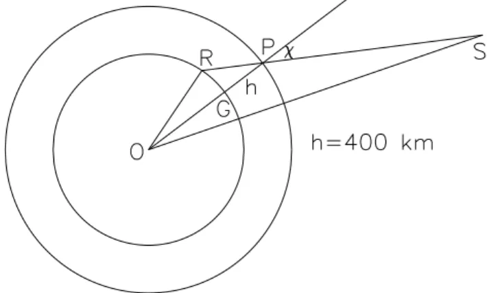
Fig. 1. Geometry of a GPS satellite (S), the ionosphere, and a
re-ceiver (R). While the total electron content is retained, the iono-sphere is assumed to be a screen iono-sphere lying at the height of 400 km from the ground. Here, P represents the intersection of the line of sight and the ionosphere, χ is zenith angle.
ambiguity in the phase measurement, TECsll from the dif-ferential phase is a relative value, but it has higher precision than TECslp. To retain phase path accuracy for the slant path TECsl, TECsll are fitted to TECslp, introducing a baseline,
Brs , for the differential phase related TECsll (Mannucci et al., 1998; Horvath and Essex, 2000)
TECsl =TECsll+Brs. (3)
If having N measurements, the baseline Brs in this paper is
computed as the average difference between pseudorange-derived TECslpi and phase-derived TECslli over the index i from i = 1 to i = N inclusive. Brs= PN i=1(T ECslp i −T ECsll i)sin2αi PN i=1sin2αi , (4)
where the square sine of the satellite’s elevation αi is
in-cluded as a weighting factor, as the pseudorange with low elevation angle is apt to be affected by the multipath effect and the reliability decreases. Consequently, the contribution to the baseline determination is greatly depleted from slant paths with low elevations. When making the above calcula-tion of Brs, a data-processing step is included to identify
pos-sible cycle-slips in either L1or L2phase measurements (Ble-witt, 1990). Thus, this study works with pseudorange-leveled carrier phases that are free of ambiguities and have lower noise and multipath effects than the pseudoranges. With a 30-s time series of dual GPS data, this part of the process is done for each pair of satellite receivers independently. All effects on the phases and pseudoranges that are common to both frequencies (such as distance of receiver satellite, clock offsets, tropospheric delay, etc.) of the obtained slant path TECsl are removed, but frequency-dependent effects, like multipath and the differential instrumental biases in the satel-lite and the receiver, are still present.
To convert to a vertical TEC from a slant path TECsl, the ionosphere is assumed to be a thin screen shell encircling
Fig. 2. Dual frequency receivers of GEONET distributed
nation-wide. The dash lines separate the area enclosed into 32 meshes. The size of the mesh is 2◦by 2◦in longitude and latitude, respec-tively.
the Earth and its center is assumed to be the same as that of the Earth. The geometry of the GPS satellite, receiver and the ionosphere is shown in Fig. 1. The intersection of the slant path from the satellite (S) to the receiver (R) through the ionosphere is referred to as a piercing point (P ). The zenith angle χ is expressed as the following
χ =arcsinREcos α
RE+h
, (5)
where α is the elevation angle of the satellite, REis the mean
radius of the Earth, and h is the height of the ionospheric layer, which is assumed to be 400 km in this paper. Further, setting satellite and receiver biases as bsand br, respectively,
then the vertical TEC is
TEC = (TECsl−bs−br)cos χ . (6)
The determination of the absolute TEC and the instru-mental biases will be described following an introduction of GEONET, a dense GPS receiver network in Japan.
2.2 GEONET in Japan and mesh division
GEONET is a GPS Earth Observation Network set up by the Geographical Survey Institute (GSI) of Japan. It has more than 1000 GPS receivers spread over Japan (Miyazaki et al., 1997), about 209 of which give precise code pseudoranges
at both frequencies. As shown in Fig. 2, the nationwide dis-tributed receivers form a sufficiently dense network, cover-ing an area from 27◦N to 45◦N and from 127◦E to 145◦E
in geographical latitude and longitude, respectively.
Also shown in the map of Fig. 2 are 32 meshes drawn with dashed lines, in which TEC should be evaluated inde-pendently. Each mesh is 2◦by 2◦in longitude and latitude, respectively. There are as many as 20 receivers in some of the meshes. There are several meshes with no receivers within. The TEC at these meshes can be obtained as well, because there are receivers in their adjacent meshes, and the piercing points spread widely depending on the satellite location and the numbers of satellites.
2.3 Determination of TEC and instrumental biases Without employing a complex mathematical model, it is as-sumed in this study that the vertical is identical at any point within a mesh, but TECs for different meshes can differ. This means that the TEC is taken to be local time-independent within 8 min, if converting the mesh width of 2◦in longitude to local time. Hence, for those lines of sight converging on the same mesh, the vertical components of their slant path TECs are all taken to be the same. It is also assumed that the satellite and receiver biases do not vary within one day.
For the line of sight from satellite j to receiver k pierc-ing through the ionosphere in mesh m at time t , referrpierc-ing to Eq. (6), we can write the following equation
sec χj kTECi+bs j+br k =TECsl j k (7)
where i denotes the order of the measurement at time t . The unknowns in Eq. (7) are TECi, bs j, and brk. With 28
satel-lites, 209 receivers, using observations with 15 min interval, the absolute TEC at 32 meshes for one day, 3300 unknowns in total, can be estimated by solving the following set of equations expressed in matrices
... . ... ... . ... 0.0 secχj k0.010.010.0 ... . ... ... . .., ... · TEC1 . TEC1 bs1 . bsJ br1 . brK = . . TECsl j k . . , (8)
where the vector on the right-hand side consists of the slant path TECsl. The number of the TECslin the vector is L. The vector on the left-hand side denotes unknowns of the TECi, the satellite bias bsj, and the receiver bias brk. The number
of the unknowns is I + J + K. The matrix on the left-hand side of Eq. (8) consists of coefficients, secχ for TEC, 1 for
bs, 1 for br and 0. It has (I + J + K) × L elements. For one
day, for each mesh there are 96 values of TEC, for 32 meshes the number of unknown TECs is 96 × 32, that is I = 3072;
J = 28, representing 28 satellites; k = 209, being the re-ceiver number. Because it is not possible to determine unam-biguously all the satellites and receiver biases absolutely, one
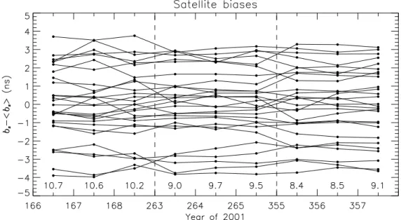
Fig. 3. GEONET derived satellite biases for 9 days over a six-month time span, where the relative bias referring to the bias with the mean of
the day removed is shown. The mean of the satellite biases are shown in the lower part of the panel. Vertical dashed lines divide inconsecutive days.
of them (normally one receiver) is set to be 0, as a reference. Then with a least-squares fitting technique, the solution to the above set of equations can be obtained by the singular value decomposition (SVD), which avoids unrealistic solutions of the equation system (Press et al., 1992). In our practical cal-culation, the number of equations is about 35 000. It takes about 8 h to carry out the whole process, from reading the GPS data to solving the Eq. (8), by a personal computer (PC) using a Pentium 4 processor.
3 Results of an application of the method
In order to demonstrate the performance of the technique, several days around the solstice and equinox period of 15– 17 June, 20–22 September, and 21–23 December 2001 were selected, before and during which it is geomagnetically quiet (Kp <4). With the procedure described above,
instrumen-tal biases and vertical absolute TEC over Japan for each day are obtained. The selected reference receiver is located at 34.16◦N, 135.22◦E, which has more than 10 receivers sur-rounding it in the same mesh.
3.1 Instrumental biases
Figure 3 shows the estimated satellite biases for the 9 days over a six-month time span, as a function of the day of year. The vertical dashed lines divide the inconsecutive days. Here, the biases are those relative to their means that are indi-cated in the lower part of the panel. For all the satellites each day, the mean of their biases is first computed, and this mean is then subtracted from each individual satellite bias (Coco et al., 1991).
Consequently, the systematic trends, such as changes in the reference receiver bias, have been removed from the satellite. Although the mean of the satellites biases decreased several ns (1ns = 2.853TECU, 1TECU = 2.853×10¹⁶e/m2) from the summer to the winter, the relative biases are quite stable. Among satellite bias differences between inconsecu-tive days, even the largest value was about 1 ns. The standard deviation in bias was from 0.076 ns to 0.664 ns for the satel-lite biases for the 9 days. It is less than 0.5 ns for 19 of the 28 satellites. So, the day-to-day variation was very small for satellite biases.
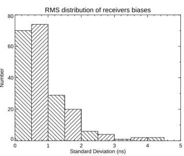
The day-to-day variation of the estimated receiver biases was also small for most of the receivers. The distribution of the standard deviation of the receiver biases to the 9-day mean is shown in Fig. 4. The greatest value was about 4 ns. Sixty-nine percent of the receivers had a standard deviation in bias that was smaller than 1 ns; 93% had less than 2 ns. In Fig. 5, a scatter diagram relates the standard deviation in re-ceiver bias for the 9 days to the geographical position of the receiver. It is evident that there is no latitude dependence of the receiver bias variation. This implies that ionospheric lo-cal characteristics have little effects on the instrumental bias determination. In spite of this, it is noticeable in Fig. 4 that there are several receivers (in mid-latitudes) with large day-to-day variation of biases. There might be several reasons for this, for example: (1) the unstableness in the receiver circuit itself; (2) bias variation of the reference receiver; (3) multi-path effects. It is likely that the unstableness in the receiver is the most reasonable explaination, because the bias variation of the reference receiver would affect all the other receivers, and the multipath effects would not vary greatly day by day.
Table 1. The standard deviation of residual (χg) from the GEONET-based method for the 9 days in 2001. The numbers in the first row refers
to the day of year 2001. The unit of χgis in TECU
DOY 166 167 168 263 264 265 355 356 357 χg 3.99 7.94 4.24 3.59 2.81 51.43 3.05 2.76 2.57
RMS distribution of receivers biases
0 1 2 3 4 5 Standard Deviation (ns) 0 20 40 60 80 Number
Fig. 4. Distribution of the standard deviation of the GEONET
de-rived receiver biases from the 9-day mean. 93% of the cases are within 2 ns.
3.2 GPS-derived TEC
With the method described in Sect. 2, TEC over Japan can be determined at the same time as the instrumental biases. 15-min time series of TEC is shown in the top panel of Fig. 6 for the 9 days from the summer to winter of 2001, for a mesh at (35◦N, 139◦E). The vertical dashed lines separate incon-secutive days. In addition to diurnal features, seasonal varia-tion is conspicuous. Data obtained by other observavaria-tion tech-niques are useful for a verification of the GPS-derived TEC. Bottom-side sounding by ionosonde is operated routinely ev-ery 15 min at Kokubunji (35.7◦N, 139.5◦E). The value foF2,
shown in the middle panel in Fig. 6, is used to evaluate the ac-curacy of the GPS-derived TEC. As is evident, the behavior of TEC is strikingly similar to that of the foF2. The variation in TEC and foF2 shows a high degree of conformity. This is also obvious for fine structures that are displayed in the daytime. These facts indicate that the GPS-derived TEC is mainly contributed from electrons in the F2-region. A more detailed comparison, the ratio of TEC to the square of foF2, is presented in the bottom panel of Fig. 6 for the 9 days. The diurnal and seasonal variation is clearly displayed. While the daytime level of the ratio is not much different from the summer to the autumn, it doubles in the winter, suggesting a greater contribution from the plasmaspheric electron content. Figure 7 shows contour maps of TEC over Japan in the
Latitude dependence of day-to-day variation
26 28 30 32 34 36 38 40 42 44 46 Latitude (deg.) 0 1 2 3 4 5 RMS of receiver bias (ns)
Fig. 5. Latitude variation of the standard deviation of the GEONET
derived receiver biases from the 9-day mean. No systematic trend can be found.
summer, the autumn and the winter of 2001. The TEC distri-bution has a simple pattern in the summer. The daytime TEC in the autumn has both a larger value and a larger gradient in latitude than that in the summer. It is even larger in the winter than that in the autumn. The nighttime TEC value in the winter is about half of that in the other two seasons. 3.3 Accuracy evaluation of the method
The standard deviation of the data from the fitting parame-ters (residuals) is used to measure how well the estimated parameters agree with the data (Bevington, 1969)
χg= v u u t L X i=1
(TECsl j k−secχj kTECi−bs j−br k)2/(L −4), (9)
where L is the number of the slant path TECsl data (refer to Sect. 2.3). Table 1 lists the χg values for the 9 days
an-alyzed. χg is less than 5 TECU for 7 days. It is about
8 TECU on 16 June 2001 (167). χg is about 51 TECU
on 22 September 2001 (265). Individual residual for each data point is examined for the day 265, on which χg is
ex-tremely large. On this day the number of slant path TECsl data used is 47 400. There are 12 991 data satisfying that
|TECsljk−secχjkTECi−bsj−brk| < 1; there are 23 695 data that |TECsljk−secχjkTECi−bsj−brk|<2. There are 40 539 data satisfying |TECsljk−secχjkTECi−bsj−brk|<
Ionospheric parameter at (139.00, 35.00) 166 167 168 263 264 265 355 356 357 0 50 100 TEC (TECU) 166 167 168 263 264 265 355 356 357 0 10 20 foF2 (MHz) 166 167 168 263 264 265 355 356 357
Day of year 2001 (UT) 0 0.5 1 1.5 TEC/(foF2) 2 (TECU/MHz 2 )
Fig. 6. A 15-min time series of TEC
at 35◦N, 139◦E for 9 days over a six-month time span. Vertical lines divide inconsecutive days. Also shown are 15-min time series of foF2, the ration of TEC to the square of foF2.
40 30 24 20 16 12 8 4 0 LST 120 100 80 70 60 50 50 40 40 30 30 20 20 10 10 2001/12/21 - 2001/12/23 40 30 La tit ud e (d eg .) 24 20 16 12 8 4 0 90 80 60 50 40 40 30 30 30 20 20 20 2001/09/20 - 2001/09/22 40 30 24 20 16 12 8 4 0 30 20 50 40 30 2001/06/15 - 2001/06/17 100 Winter Autumn Summer
Fig. 7. Ionospheric distribution over Japan in the summer, the autumn, and the winter of 2001. Contours are la-beled in units of TECU and the spacing is 10 TECU.
5, that is to say the fitting results agree well with most of the data. Furthermore, it is found that most of the large residu-als are from those meshes at latitudes lower than 35◦; among
1233 data yielding |TECsljk−secχjkTECi−bsj−brk|<10, there are 950 data are from meshes at latitudes lower than 35◦. It is probable that a steep latitude gradient in the low lat-itude ionosphere, created by the development of an equatorial anomaly in equinox, caused the large standard deviation in the fitting on day 265. Thus, the large residuals mainly come from the TEC gradient within meshes at lower latitudes. A large χg, however, does not necessarily mean the low fitting
accuracy of the instrumental biases; the estimated satellite biases on day 265 do not differ very much from those on day 264, as seen in Fig. 3. A comparison of the receiver biases on the two days is shown with a scatter plot in Fig. 8. The cir-cles in the figure represent those receivers located at latitude 35◦, and the crosses refer to the receivers at latitudes ≤35◦.
The agreement between the biases for the two days is very good, regardless of the receiver latitude, although moderate deviation can be found for a few receivers. Thus, even for the worst case in terms of residual, the method determines the instrumental biases with a high accuracy.
4 Estimation of bias for a single receiver
The method described in the above section is not always ap-plicable to any situation, because the technique is based on a highly dense receiver network in a small area. Also, the algorithm requires a lengthy processing time, which does not meet the requirement of monitoring the ionosphere in nearly real-time. However, once the satellite biases are de-termined by using GEONET, those values can be commonly used in any other location in the globe, even where a single receiver is installed. This section will describe a simple and fast method to estimate the bias of a single receiver using the satellite biases determined by GEONET, and the accuracy of the simple method will be evaluated.
4.1 A simple method
Generally, one GPS receiver simultaneously receives signals from 5 or more GPS satellites at any time. The elevation angle of those satellites could vary widely. The piercing points would be scattered widely but within a limited area, roughly 23◦ in longitude and 32◦ in latitude, with the
re-ceiver at the center. From different satellites with different elevations the lines of sight to the receiver lead to a spatial variation of slant path TECslat any observation time. If the ionosphere is horizontally homogeneous and instrumental bi-ases are correctly removed, the vertically converted TECs should be identical for all of the satellites. In an actual case, in which the ionosphere has a horizontal gradient and vertical structure, the scattering of vertical TECs is assumed to be the smallest when the instrumental biases are correctly removed. As the satellite biases are well determined by GEONET and shown to be stable (refer to Sect. 3), which are known values
Fig. 8. Comparison of GEONET derived receiver biases on day 265
with those on day 264. As shown in the figure, the circles represent those receivers located at latitude 35◦ or lower than 35◦, and the crosses refer to the receivers at higher latitudes. No matter where the receivers are, both circles and crosses gather along the diagonal, showing a nice agreement between receiver biases estimated on the two different days.
hereafter, the receiver bias is estimated independently from GEONET by trying out a series of bias candidates and find-ing the one that gives a minimum deviation of TECs to their mean. In a mathematical description, given a trial receiver bias b(i), the standard deviation of TECs to their mean is calculated at each observation time. Then, the total standard deviations, 6σi, is obtained for the whole day. The value of b(i0)when 6σitakes the minimum value, 6σi, is considered
to be a correct receiver bias (hereafter, referred to as fitted re-ceiver bias). It takes only several minutes to obtain the fitted receiver bias by a personal computer (PC) using a Pentium 4 processor.
When different receiver biases are applied, the dispersion of vertical TECs is examined by using actual data set. For the convenience of comparison, one receiver is chosen from GEONET, which is located at 35.53◦N, 137.89◦E. The re-sults for the observations on 17 June 2001 are given in Fig. 9. The dashed lines are for slant path TECslfrom the satellites
to the receiver. The solid lines represent vertically converted TECs after the satellite and receiver biases are removed. For the three panels, the satellite biases were identical and deter-mined with the method described in Sect. 3, but the receiver bias was taken to be different: in the top panel, the receiver bias is a GEONET-derived one; in the lower two panels, the receiver biases were arbitrarily chosen so that it is much less than the GEONET-derived one in the middle panel, and much larger than the GEONET-derived one in the bottom panel. The corresponding value of 6σi for each case is shown at
Fig. 9. Slant path TECsl (dash lines)
from GPS satellites to a receiver at 35.53◦N, 137.89◦E. The solid lines are vertical TEC converted from TECsl
with the instrumental biases removed. The satellite biases are GEONET de-rived. The receiver bias is GEONET derived in the top panel. They are as-sumed values in the lower two panels. The one-day sum of the standard devia-tion of TECs to their mean at any time, 6σ, is shown in each panel.
Fig. 10. Fitted bias to a receiver at 35.53◦N, 137.89◦E. The GEONET derived bias value, 2.29 ns, is also given.
receiver bias is applied, the curves do not converge.
Figure 10 shows the variation of 6σias a function of b(i)
for the same data set. From the figure the receiver bias is determined as 2.78 ns, which is close to the value determined from GEONET, 2.29 ns. The difference between biases from the two methods is only 0.49 ns.
4.2 Accuracy of the simple method
The same procedure was applied to all the GEONET re-ceivers, and the receiver biases derived from the two methods are compared. A scatter plot of the GEONET-derived bias versus the fitted bias on 17 June 2001 is shown in Fig. 11 for all receivers. The agreement between the GEONET br and
the fitted one is amazingly good. Figure 12 gives the distri-bution of the difference between the GEONET and the fitted biases, 1br(= br GEONET−br f it)(hereafter, refered to as
an error of fitted bias or simply an error) for the same data set. It can be seen that for most of the receivers (93%), the errors are within ±2 ns.
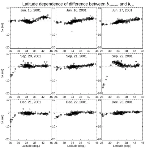
Table 2 summarizes the percentage of the number of re-ceivers for which the errors are within ±2 ns for the 9 days analyzed. It is noticeable that on 22 September 2001 (the 265th day of the year) the fitted bias has a large error for about 1/3 of the receivers. Specifically, these receivers are located at latitudes lower than 35◦N, as shown in Fig. 13, where the error’s latitude dependence for the other days is also displayed. This is in agreement with the large χg on
the day 265 discussed in Sect. 3.3. On the whole, the value of br f it tends to be larger than that of br GEONET for the receivers at lower latitudes (<30◦N), and the error tends to
Table 2. The percentage of the difference within ±2 ns between the GEONET derived receiver bias and single receiver fitted bias. The
numbers in the first row refer to the day of year 2001
DOY 166 167 168 263 264 265 355 356 357 Perc. 79% 91% 93% 90% 95% 69% 93% 94% 98% -30 -20 -10 0 10 20 30 40 br_GEONET (ns) -30 -20 -10 0 10 20 30 40 br_fit (ns) Jun. 17, 2001
Fig. 11. Singly fitted bias is plotted versus GEONET derived bias
for all receivers on 17 June 2001. The relationship br GEONET =
br f itis also shown for comparison.
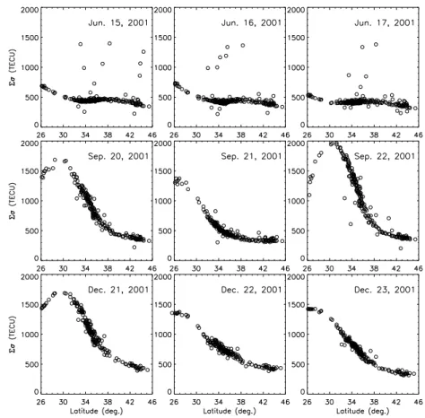
increase with the decrease in latitude. This suggests that the ionospheric condition affects the bias determination by fit-ting for a single receiver. For further investigation of the error source, and hence, the limit in the application of the method, the total standard deviation of the TECs to their mean, 6σ , for each receiver was calculated by using the fitted receiver bias. The latitude variations of 6σ are shown in Fig. 14. By comparing Figs. 13 and 14, it can be seen that a large value of 6σ , or ill convergence, does not necessarily yield a large error. Taking 22 September 2001 as an example, the er-ror decreased with the increase in 6σ at latitudes lower than 30◦N.
The latitude dependence of the 6σ and hence, the bias er-ror can be explained in terms of the TEC latitude gradient and the equatorial anomaly, which are clearly depicted in Fig. 14. Having high activity in the equinox, the equatorial anomaly is characterized by two electron density peaks (known as crest) in the vicinity of the geomagnetic latitude 15◦ symmet-ric to the geomagnetic equator, which corresponds to about 25◦N geographically at Japan’s longitude. For a receiver lo-cated at or near the crest of a equatorial anomaly, the satel-lites within the range tend to be distributed apart from the crest. The vertically converted TECs would have a mean smaller than the TEC through the crest. And the deviation
Distribution of difference between br_GEONET and br_fit
-6 -5 -4 -3 -2 -1 0 1 2 3 4 5 6 br_GEONET-br_fit (ns) 0 10 20 30 40 50 60 70 80 90 Number Jun. 17, 2001
Fig. 12. Distribution of the number with the difference between
GEONET derived bias and fitted bias for all receivers on 17 June 2001.
of TECs from their mean, 6σ , would be smaller than that of TECs with large latitude gradient or variance.
5 Summary
The dual GPS data from 209 GEONET receivers in Japan was used to determine TEC over Japan, as well as the biases of satellites and receivers. The paper also proposed a faster and simpler way to estimate a single receiver’s bias as long as the satellite biases are known. The methods described herein have been applied to geomagnetically quiet days in the sum-mer, the autumn and the winter.
The main results obtained in the biases’ estimation can be summarized as follows:
1. The standard deviation from the mean is from 0.076 ns to 0.664 ns for the 28 GPS satellite biases for 9 days over the six-month time span.
2. Ninety-three percent of the receiver biases have a stan-dard deviation that is smaller than 2 ns from the mean for the 9 days. It can be as large as 4 ns for a few re-ceivers.
3. The fitted bias for a single receiver is generally within
26 30 34 38 42 46 -20 -10 0 10 ∆ br (ns) Jun. 15, 2001 26 30 34 38 42 46 -20 -10 0 10 Jun. 16, 2001 26 30 34 38 42 46 -20 -10 0 10 Jun. 17, 2001 26 30 34 38 42 46 -20 -10 0 10 ∆ br (ns) Sep. 20, 2001 26 30 34 38 42 46 -20 -10 0 10 Sep. 21, 2001 26 30 34 38 42 46 -20 -10 0 10 Sep. 22, 2001 26 30 34 38 42 46 Latitude (deg.) -20 -10 0 10 ∆ br (ns) Dec. 21, 2001 26 30 34 38 42 46 Latitude (deg.) -20 -10 0 10 Dec. 22, 2001 26 30 34 38 42 46 Latitude (deg.) -20 -10 0 10 Dec. 23, 2001
Latitude dependence of difference between br_GEONET and br_fit
Fig. 13. Latitude dependence of the difference between biases determined from the two different methods for the 9 days analyzed. The
dashed line referring to no difference is plotted in each panel for easy comparison.
from a GEONET derived bias tends to occur for those receivers at lower latitude (<35◦N) in the autumn and winter. This is the result from the steep latitude gradient in the local ionosphere, probably with the development of the equatorial anomaly effects.
Concerning the GPS-derived TEC, the following has been found from a comparison with foF2:
1. The diurnal and seasonal variations in TEC and foF2 show a high degree of conformity.
2. The ratio of TEC to the square of foF2 also showed di-urnal and seasonal variation. The daytime peak value in the winter was about twice that in the summer and autumn.
6 Conclusions
It can be concluded based on the results of an analysis of data obtained from GEONET that the method described herein is efficient and qualified for use to derive the absolute TEC, and to determine the biases of GPS satellites and receivers. Since the day-to-day variation is small in satellite and receiver bi-ases, it is only necessary that the instrumental biases be
esti-mated or calibrated from time to time. This is especially true for satellite biases.
The proposed method for estimating a single receiver’s bias is faster and sufficiently accurate for a receiver at mid-latitude. It has the potential to meet the requirement of being able to monitor the ionosphere in nearly real-time. It can be also applied to the receiver far from a GPS network. But the accuracy of a fitting bias can be low for a receiver at a lower latitude, due to the effects of equatorial anomaly. This dis-advantage can be avoided by determining the receiver bias at mid-latitude before its establishment at a lower latitude.
The GPS-derived TEC is mainly contributed from the elec-trons in the F2-region. It is shown from the ratio of TEC to the square of foF2 that plasmaspheric electron content is larger in the winter than that in the summer or autumn.
Acknowledgements. We would like to thank the Geographical
Sur-vey Institute of Japan for convenient and free use of their GEONET GPS data. Thanks are also due to A. Saito, K. Hocke and Y. Otsuka for helpful discussions.
Topical Editor M. Lester thanks two referees for their help in evaluating this paper.
Fig. 14. The variation of 6σ with latitude for the 9 days analyzed.
References
Blewitt, G.: An automatic editing algorithm for GPS data, Geophys. Res. Lett., 17, 199–202, 1990.
Bevington, P. R.: Data reduction and error analysis for the physical sciences, Mcgraw-Hill, New York, 1969.
Coco, D. S., Coker, C., Dahlke, S. R., and Clynch, J. R.: Variabil-ity of GPS satellite differential group delay biases, IEEE Trans. Aerosp. Electron. Sys., 27, 931–938, 1991.
Ho, C. M., Mannucci, A. J., Sparks, L., Pi, X., Lindqwister, U. J., Wilson, B. D., Iijima, B. A., and Reys, M. J.: Ionospheric total electron content perturbations monitored by the GPS global net-work during two northern hemisphere winter storms, J. Geophys. Res., 103, 26 409–26 420, 1998.
Hovath, I. and Essex, E. A.: Using observations from the GPS and TOPEX satellites to investigate night-time TEC enhancements at mid-latitudes in the southern hemisphere during a low sunspot number period, J. Atmos. Sol. Terr. Phys., 62, 371–391, 2000. Lanyi, G. E. and Roth, T.: A comparison of mapped and measured
total ionospheric electron content using Global Positioning Sys-tem and beacon satellites observations, Radio Sci., 23, 483–492, 1988.
Lunt, N., Kersley, L., and Bailey, G. J.: The influence of the protonosphere on GPS Observations: Model simulations, Radio Sci., 34, 3, 725–732, 1999.
Mannucci, A. J., Wilson, B. D., Yuan, D. N., Ho, C. H., Lindqwis-ter, U. J., and Runge, T. F.: A global mapping technique for GPS-derived ionospheric electron content measurements, Radio Sci., 33, 565–582, 1998.
Miyazaki, S., Saito, T., Sasaki, M., Hatanaka, Y., and Iimura, Y.: Expansion of GSI’s nationwide GPS array, Bull. Geogr. Surv. Inst., 43, 23–34, 1997.
Otsuka, Y., Ogawa, T., Saito, A., Tsugawa, T., Fukao, S., and Miyazaki, S.: A new technique for mapping of total electron content using GPS network in Japan, Earth Planets Space, 63– 70, 2002.
Press, W. H., Teukolsky, S. A., Vetterling, W. T., and Flannery, B. P.: Numerical Recipes in Fortran 77, Cambridge University Press, 670–673, 1992.
Reiff, P. H.: The use and misuse of statistical analysis, (Eds) Carovillano, R. L. and Forbes, J. M., Solar-Terrestrial Physics, 493–522, 1983.
Sard`on, E., Rius, A., and Zarraoa, N.: Estimation of the transmit-ter and receiver differential biases and the ionospheric total elec-tron content from Global Positioning System observations, Radio Sci., 29, 577–586, 1994.
Sard`on, E. and Zarraoa, N.: Estimation of total electron content using GPS data: How stable are the differential satellite and re-ceiver instrumental biases? Radio Sci., 32, 1899–1910, 1997. Wilson, B. D., Mannucci, A. J., Edwards, C. D., and Roth, T.:
Global ionospheric maps using a global network of GPS re-ceivers, paper presented at the international Beacon Satellite Symposium, MIT, Cambridge, MA, July 6-12, 1992.
Wilson, B. D., Mannucci, A. J., and Edwards, C. D.: Subdaily northern hemisphere ionospheric maps using an extensive net-work of GPS receivers, Radio Sci., 30, 639–648, 1995.