HAL Id: hal-00489506
https://hal.archives-ouvertes.fr/hal-00489506
Submitted on 5 Jun 2010
HAL is a multi-disciplinary open access
archive for the deposit and dissemination of
sci-entific research documents, whether they are
pub-lished or not. The documents may come from
teaching and research institutions in France or
abroad, or from public or private research centers.
L’archive ouverte pluridisciplinaire HAL, est
destinée au dépôt et à la diffusion de documents
scientifiques de niveau recherche, publiés ou non,
émanant des établissements d’enseignement et de
recherche français ou étrangers, des laboratoires
publics ou privés.
ICA-based sparse feature recovery from fMRI datasets
Gaël Varoquaux, Merlin Keller, Jean Baptiste Poline, Philippe Ciuciu,
Bertrand Thirion
To cite this version:
Gaël Varoquaux, Merlin Keller, Jean Baptiste Poline, Philippe Ciuciu, Bertrand Thirion. ICA-based
sparse feature recovery from fMRI datasets. Biomedical Imaging, IEEE International Symposium on,
Apr 2010, Rotterdam, Netherlands. pp.1177. �hal-00489506�
ICA-BASED SPARSE FEATURES RECOVERY FROM FMRI DATASETS
Ga¨el Varoquaux
1,2, Merlin Keller
1,2, Jean-Baptiste Poline
2, Philippe Ciuciu
2, Bertrand Thirion
1,2 1Parietal project team, INRIA, Saclay-ˆIle de France, Saclay, France,
2
CEA, DSV, I
2BM, Neurospin, Saclay, France
ABSTRACT
Spatial Independent Components Analysis (ICA) is increas-ingly used in the context of functional Magnetic Resonance Imaging (fMRI) to study cognition and brain pathologies. Salient features present in some of the extracted Independent Components (ICs) can be interpreted as brain networks, but the segmentation of the corresponding regions from ICs is still ill-controlled. Here we propose a new ICA-based pro-cedure for extraction of sparse features from fMRI datasets. Specifically, we introduce a new thresholding procedure that controls the deviation from isotropy in the ICA mixing model. Unlike current heuristics, our procedure guarantees an exact, possibly conservative, level of specificity in feature detec-tion. We evaluate the sensitivity and specificity of the method on synthetic and fMRI data and show that it outperforms state-of-the-art approaches.
Index Terms— ICA, fMRI, ROC, sparse models.
1. INTRODUCTION
In neuro-imaging, ICA is the most popular method to ex-plore the spatial correlation structure of fMRI signals. Some extracted ICs match well-known brain networks [1, 2] and have been shown to correspond to units targeted by neuro-degenerate diseases [3]. These sources form spatial maps that represent sparse networks of brain activity: only a small per-centage of the voxels observed are active in a given network. Daubechieset al. [4] have argued that this sparsity is key to the success of ICA in the context of fMRI. When applied to data generated from sparse sources, ICA amounts to sparse coding [5]. It has enjoyed more success in the neuro-imaging community, probably because it groups together correlated features into components interpreted as brain networks. Cur-rent state-of-the-art ICA models for fMRI (MELODIC [2]) apply univariate mixture models to ICs to separate signal from noise and recover the sparse structure.
In this paper, we present a multivariate model of sparse brain activity and an associated procedure for recovering the sparse features with a statistical control of false detections in the presence of noise. We will focus on single-subject
analy-Funding from INRIA-INSERM collaboration.
sis but the method could easily be extended to group analysis with the addition of a group model.
2. SIGNAL MODELING AND ESTIMATION ICA is an unsupervised learning algorithm. As such, it does not provide a framework for statistical-significance testing, but can be used to analyze fMRI data without external corre-lates, such as in resting state. We introduce a model of the fMRI signal based on the assumption of very sparse sources.
Generative model. In the observations from the scanner
Y1, the underlying BOLD dynamics is confounded by obser-vation noise F. As with most fMRI ICA analysis procedures, we assume that the signal of interest spans only a sub-space of the observation space. Components C spanning this sub-space can be estimated using probabilistic principal compo-nent analysis (PCA) [2], which assumes F to be Gaussian-distributed, and lying in a subspace orthogonal to C:
Y= W C + F, (1)
where Y and F are(ntime steps, nvoxels) matrices, the rows of
which form pattern vectors. C is the(ncomponents, nvoxels)
pat-tern matrix of the retained principal components and W is the matrix of their loadings in the observed signal. In this paper, we do not discuss estimation of the sub-space of interest, but focus on recovering sparse brain-activity sources from C.
We model the patterns C as generated by a set of sources
A, confounded by additive noise E, and observed as a linear
mixture in the sub-space spanned by C:
C= M B (2) B= A + E (3)
M is an orthogonal mixing matrix, A, B, and E are (ncomponents, nvoxels) matrices. Unlike F, E is in the same
sub-space as the brain sources. In addition, we assume that the true sources correspond to the marginals Ai that are sparse: most of the coefficients of Aiare zeros. As a result, the histogram of Aiis strongly super-Gaussian: it has heavy tails. If the amplitude of the noise E is small compared to the non-zero coefficients of A, B is also super-Gaussian and can
1Y corresponds to the data from the scanner after slice-timing
interpola-tion and mointerpola-tion correcinterpola-tion. In addiinterpola-tion, when doing group analysis, a normal-ization procedure is often applied, followed by Gaussian spatial smoothing.
be estimated from C using ICA. We use FastICA, a proce-dure that selects a basis of the signal sub-space maximizing non-Gaussianity of the corresponding marginal distributions [6].
If the components B are observed mixed, the observed projections Ci reflect mostly the isotropic noise E and not the sources of interest A that are sparse only in a particular basis. This is why the estimation of the mixing model (2) is important for fMRI data analysis, as the marginals on the estimated basis separate A from the background noise E.
Thresholding ICs to control for noise. We assume that the values of the non-zero voxels of sources A are larger than the standard deviation σ of E. According to our model, select-ing voxels specific of the support of A amounts to choosselect-ing a threshold ταto apply on the ICs ˆB. ICA estimates particular directions of the feature space, thus a possible null hypothesis
H0for ICA is that all directions are equivalent. As a result, the null distribution for the marginals Aiis given by projec-tions on random direcprojec-tions ω of the feature space.
p(Ai> τα|H0) = mean ω,||ω||=1p(|ω
TB| > τ
α) (4) We can sample this distribution directly from the data. In addition, ωTB is a linear combination of the random variables
Bi. As the sub-space has been whitened by the PCA, they all
have a variance of 1. For high dimensions, the central limit theorem thus states that the distribution of ωTB is Gaussian
of variance 1. In this case, the p-value is given by the inverse of the cumulative distribution function of a Gaussian process, and the threshold can be set as with a normal null.
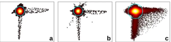
A representation of the signal in feature space is given on Fig. 1 for various distributions: synthetic data generated from the model exposed above (Fig. 1a), synthetic data with additional super-Gaussian noise, (Fig. 1b), and fMRI data (Fig. 1c). All share a central mode corresponding to E in our description, that can be approximated as a multivariate Gaus-sian process. In addition, for each mixing direction, activated voxels can be found when moving away from the center.
Our model is different from most noisy ICA models, as they assume that contribution of the noise to the signal sub-space is small. They account for the noise in the ICA estima-tion by correcting the bias it introduces to the whitening and the measures of statistical independence [7]. In our model, noise accounts for a large fraction of the variance in the sig-nal sub-space.
3. SIMULATION STUDY
We generate synthetic samples ˜Y from our model with a
known ground truth and noise model. We consider 9 features
˜
A, that is 2D maps (80, 80) pixel large and made of one
or two rectangles of uniformly-active pixels on a null back-ground. We add random noise ˜E generated by a multivariate
normal distribution of isotropic variance 1. We control the
a b c
Fig. 1. Scatter plot of samples projected in the subspace spanned by the two first ICs identified. The density is rep-resented by a colormap ranging from black (low density) to white (high density). The threshold as set by the model with
p= 10−2is represented as a light blue circle.(a)Simulated data with 9 features total, with E generated from a Gaussian process with σ = 0.15. (b) Same simulations with super-Gaussian noise (kurtosis of4).(c)fMRI data.
amplitude of the noise with a parameter λ: ˜B= ˜A+ λ ˜E.
We draw a random rotation matrix ˜M to mix the patterns ˜B,
and apply a Gaussian spatial smoothing of FWHM 2 pixels to simulation the point spread function of the scanner. Due to the smoothing, the noise term is observed as a random Gaussian field with a reduced variance compared to the initial random process. We set λ to control the variance of this field. In addition, as it is likely that, in real fMRI settings, not all background noise can be described by Gaussian processes, we generate synthetic data with non-Gaussian noise. For this, in addition to the previous Gaussian random field, ˜Eg, we gen-erate a super-Gaussian contribution ˜Eng by applying a non-linear rescaling to a smoothed Gaussian random field. We use the cubic non-linearity that generatesspikynoise with a long-tailed distribution. The additional noise term is thus sparse, and not invariant by rotation of the feature space. We add it to the signal of interest in the observation basis. We set the contributions of both noise terms to control the variance and kurtosis of the resulting random process: ˜C = ˜M ˜A+ λ(cos θ ˜M ˜Eg + sin θ ˜Eng). This structured noise term
vio-lates the noise model of the ICA algorithm and poses thus a challenge to the feature extraction by offsetting the estimation of the mixing matrix, and thus the projection.
Spatial maps generated by the simulations are presented on Fig. 2. The samples projected in feature space on the 2 first ICs are presented on Fig. 1. We apply ICA estima-tion and thresholding as described above. To quantify the specificity and the sensitivity in feature detection, we plot receiver-operator characteristics on Fig. 4 for Gaussian and super-Gaussian (kurtosis= 4) noise. Increasing noise
ampli-tude σ degrades estimation performance, as the central mode becomes indistinguishable from the outliers we are interested in. Performances are slightly degraded by the addition of the super-Gaussian noise. It induces errors in the choice of the projection basis, as can be seen on Fig. 1b: in the pro-jected space, sources are not completely unmixed. In addi-tion, on Tab. 1, we compare false positive rates to the spec-ified p-value. We find that for Gaussian noise amplitudes up to σ= 0.20 or super-Gaussian noise amplitude of σ = 0.15,
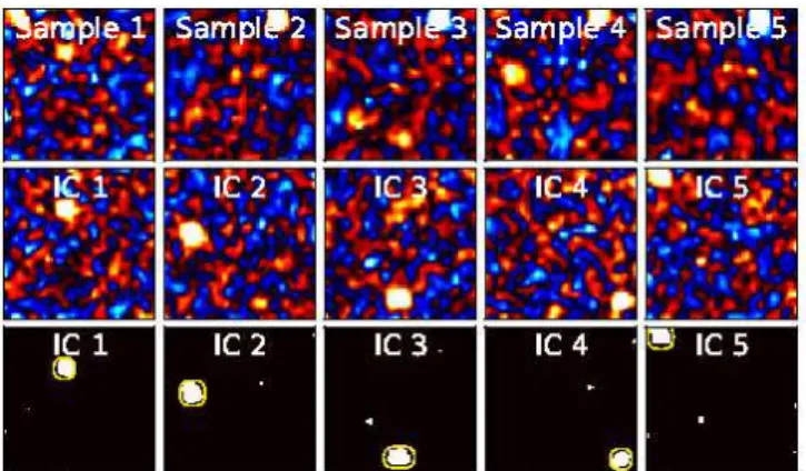
Fig. 2. Simulated data, showing 5 samples out of 9, for E generated from a super-Gaussian process with σ= 0.15 and
a kurtosis of4. The threshold is set by the model with p = 10−2. Top row: observed samples Y. Middle row: ICs
B. Bottom row: estimated sources A, the ground truth is
outlined in light yellow.
Specified p-value 5·10−2 1.0·10−2 5.0·10−3 Gaussian, σ = .15 4.0·10−2 7.1·10−3 4.0·10−3 super-Gaussian, σ = .15 4.2·10−2 1.0·10−2 6.2·10−3 Gaussian, σ = .20 4.9·10−2 9.4·10−3 5.2·10−3 super-Gaussian, σ = .20 5.2·10−2 1.3 ·10− 2 7.9·10−3 Gaussian, σ = .30 6.0·10−2 1.3·10−2 7.4·10−3 super-Gaussian, σ = .30 5.9·10−2 1.5·10−2 1.0·10−2 fMRI data 3.6·10−2 1.7·10−2 1.3·10−2 Table 1. False positive rates as a function of model-based p-value, for simulated and fMRI data.
the p-values give an exact control on type 1 errors. With more noise, the tail of the central mode cannot account for all false detections for small p-values. We stipulate that the additional errors come from projection error due to incomplete source unmixing by the ICA procedure.
4. FMRI STUDY
We apply our method to fMRI data for 12 subjects at rest from a previous study [8]. 820 volumes were acquired with a repetition time (TR) of1.5 s. We run the procedure (ICA
analysis and thresholding) for single-subject data on the first 40 principal components. For fMRI data, the ground truth is not known, so we generate degraded datasets from the origi-nal dataset, and consider the latter as a pseudo ground truth to quantify error rates. This procedure quantifies consistency of the estimator in the presence of noise. To generate degraded datasets while retaining observations of the same brain activ-ity, we use one volume out of 3. The effective TR of the down-sampled datasets is4.5 s. This sampling rate is enough to
retain most of the hemodynamic response, convolved by the 6-second-long response function. In addition, the 3 resulting interleaved time series sample different high-frequency noise
Fig. 4. ROC plot: sensitivity as a function of false posi-tive rate for synthetic data using Gaussian and super-Gaussian (kurtosis = 4) noise of varying σ, as well as for fMRI data.
that confounds the signal of interest. Thresholded ICs esti-mated on the various resampled datasets for one subject are matched with the corresponding pseudo ground truth. Fig. 3 presents pseudo ground truth and downsampled data. On non-thresholded ICs, we can see that the level of background noise is indeed higher in ICs learned on downsampled data. We run the MELODIC mixing model on the ICs to compare sensitiv-ity (false negatives) and specificsensitiv-ity (false positives).
As seen on the ROC plot (Fig. 4), average performance on fMRI data for the 12 subjects is on par with simulated data. Good control of false positives can be achieved, but the true positive rate remains limited. This can be explained by er-rors in our pseudo-ground truth. In addition, the false positive rate is controlled by the specified p-value only to10−2, al-though to account for errors in the pseudo-ground truth, the observed false positive rate should be corrected by a factor
0.5. With MELODIC’s mixture model, we specify different
inter-class mixing probability ratios to vary specificity; we do not report on very large or very small ratios as they induce non-monotonous thresholding and poor overall performance. Our multivariate thresholding proceeding can achieve better specificity/sensitivity trade off MELODIC’s mixture model.
ICs estimated on fMRI data most often display a few salient features related to anatomical regions and may be interpreted as brain networks. On such IC, both our thresh-olding procedure and MELODIC’s mixture model extract similar regions, although our procedure yields fewer small clusters outside of the main segmented areas (see Fig. 3, top). In contrast, some ICs, representative of non-cognitive pro-cesses such as blood flow or movement, are very fragmented and diffuse with no region strongly standing out. On these ICs, a mixture model fits the null distribution to the center of the histogram, and thus selects large regions, whereas our thresholding procedure selects very few voxels, as it does not consider the component by itself, but as part of the complete multivariate signal (see Fig. 3, bottom).
Pseudo ground truth MELODIC mixture model Multivariate thresholding procedure
Downsampled data
Pseudo ground truth MELODIC mixture model Multivariate thresholding procedure
Downsampled data
Fig. 3. ICs estimated from fMRI data and thresholded using MELODIC’s mixture model, and our multivariate thresholding procedure. Top rows: IC detecting the primary visual areas. Bottom rows: IC representative of a vascular artifact.
5. CONCLUSION
This contribution presents a procedure for thresholding ICA patterns of fMRI time series to recover sparse sources using a multivariate model of spatially-sparse brain activity that does not rely on correlating with external stimuli. From a practical point of view, the main improvement over existing ICA-based methods for fMRI is that non-neuronal patterns are rejected as they do not correspond to very salient features. We have val-idated on simulated data and resting-state fMRI data that the procedure can yield exact control of the false positive rates for p >10−2and achieves better sensitivity/specificity trade-offs than the current state-of-art fMRI ICA support-selection procedures. Control of false detections and consistency of es-timation on noisy data is important for clinical and medical re-search applications of resting-state fMRI. Our procedure can be understood as outlier detection with projection pursuit, as proposed by Gnanadesikan and Kettenring [9], using ICA.
6. REFERENCES
[1] M.J. McKeown, S. Makeig, G.G. Brown, et al. , “Anal-ysis of fMRI data by blind separation into independent spatial components,” Hum. Brain Mapp., vol. 6, no. 3, pp. 160–188, 1998.
[2] C. F. Beckmann and S. M. Smith, “Probabilistic indepen-dent component analysis for functional MRI,” Trans Med
Im, vol. 23, pp. 137–152, 2004.
[3] W.W. Seeley, R.K. Crawford, J. Zhou, et al. , “Neurode-generative Diseases Target Large-Scale Human Brain Networks,” Neuron, vol. 62, no. 1, pp. 42–52, 2009. [4] I. Daubechies, E. Roussos, S. Takerkart, et al. ,
“Indepen-dent component analysis for brain fMRI does not select for independence.,” Proc Natl Acad Sci U S A, vol. 106, no. 26, pp. 10415–10422, 2009.
[5] A. Hyvarinen, P. Hoyer, and E. Oja, “Sparse code shrink-age for imshrink-age denoising,” in Neural Networks Conference
Proceedings, 1998, vol. 2, pp. 859–864.
[6] A. Hyv¨arinen and E. Oja, “Independent component anal-ysis: algorithms and applications,” Neural Networks, vol. 13, no. 4-5, pp. 411 – 430, 2000.
[7] A. Cichocki, S.C. Douglas, and S. Amari, “Robust tech-niques for independent component analysis with noisy data,” Neurocomputing, vol. 22, pp. 113–130, 1998. [8] S. Sadaghiani, G. Hesselmann, and A. Kleinschmidt,
“Distributed and Antagonistic Contributions of Ongoing Activity Fluctuations to Auditory Stimulus Detection,” J.
Neurosci., vol. 29, no. 42, pp. 13410, 2009.
[9] R. Gnanadesikan and J.R. Kettenring, “Robust estimates, residuals, and outlier detection with multiresponse data,”