Venus’ upper atmosphere revealed by a GCM: I. Structure and variability of the circulation

(1)

HAL Id: insu-03162299

https://hal-insu.archives-ouvertes.fr/insu-03162299v2

Submitted on 16 Jun 2021

HAL is a multi-disciplinary open access

archive for the deposit and dissemination of

sci-entific research documents, whether they are

pub-lished or not. The documents may come from

teaching and research institutions in France or

abroad, or from public or private research centers.

L’archive ouverte pluridisciplinaire HAL, est

destinée au dépôt et à la diffusion de documents

scientifiques de niveau recherche, publiés ou non,

émanant des établissements d’enseignement et de

recherche français ou étrangers, des laboratoires

publics ou privés.

Distributed under a Creative Commons Attribution - NoDerivatives| 4.0 International

License

Venus’ upper atmosphere revealed by a GCM: I.

Structure and variability of the circulation

Thomas Navarro, Gabriella Gilli, Gerald Schubert, Sébastien Lebonnois,

Franck Lefèvre, Diogo Quirino

To cite this version:

Thomas Navarro, Gabriella Gilli, Gerald Schubert, Sébastien Lebonnois, Franck Lefèvre, et al.. Venus’

upper atmosphere revealed by a GCM: I. Structure and variability of the circulation. Icarus, Elsevier,

2021, 366 (September), pp.114400. �10.1016/j.icarus.2021.114400�. �insu-03162299v2�

(2)

Icarus 366 (2021) 114400

Available online 6 March 2021

Contents lists available atScienceDirect

Icarus

journal homepage:www.elsevier.com/locate/icarus

Research Paper

Venus’ upper atmosphere revealed by a GCM: I. Structure and variability of

the circulation

Thomas Navarro

a,b,∗

, Gabriella Gilli

c,d

_{, Gerald Schubert}

a

_{, Sébastien Lebonnois}

e

_,

Franck Lefèvre

f

_{, Diogo Quirino}

c,d

a_{Department of Earth, Planetary and Space Sciences, University of California, Los Angeles, CA, USA} b_{McGill Space Institute, McGill University, Montreal, Canada}

c_{Instituto de Astrofisica e Ciências do Espaço (IA), OAL, Tapada da Ajuda, PT1349-018 Lisboa, Portugal} d_{Faculdade de Ciências, Campo Grande, PT1749-016 Lisboa, Portugal}

e_{Laboratoire de Météorologie Dynamique (LMD) Paris, France} f_{IPSL/LATMOS, Paris, France}

A R T I C L E

I N F O

Keywords: Venus GCM Upper atmosphere Atmospheric circulation Airglow Kelvin wave Singlet oxygen

A B S T R A C T

A numerical simulation of the upper atmosphere of Venus is carried out with an improved version of the Institut Pierre-Simon Laplace (IPSL) full-physics Venus General Circulation Model (GCM). This simulation reveals the organization of the atmospheric circulation at an altitude above 80 km in unprecedented detail. Converging flow towards the antisolar point results in supersonic wind speeds and generates a shock-like feature past the terminator at altitudes above 110 km. This shock-like feature greatly decreases nightside thermospheric wind speeds, favoring atmospheric variability on a hourly timescale in the nightside of the thermosphere. A ∼5-day period Kelvin wave originating in the cloud deck is found to substantially impact the Venusian upper atmosphere circulation. As the Kelvin wave impacts the nightside, the poleward meridional circulation is enhanced. Consequently, recombined molecular oxygen is periodically ejected to high latitudes, explaining the characteristics of the various observations of oxygen nightglow at 1.27 μm. An analysis of the simulated 1.27 μmoxygen nightglow shows that it is not necessarily a good tracer of the upper atmospheric dynamics, since contributions from chemical processes and vertical transport often prevail over horizontal transport. Moreover, dayside atomic oxygen abundances also vary periodically as the Kelvin wave momentarily decreases horizontal wind speeds and enhances atomic oxygen abundances, explaining the observations of EUV oxygen dayglow. Despite the nitrogen chemistry not being currently included in the IPSL Venus GCM, the apparent maximum NO nightglow shifted towards the morning terminator might be explained by the simulated structure of winds.

1. Introduction

The circulation of the Venusian atmosphere is dominated by the westward retrograde zonal superrotation (RZS) of the cloud deck at altitudes up to 70 km. Higher up in the thermosphere, the strong day-to-night thermal gradient induces a Subsolar to Antisolar (SS–AS) circulation, with air flowing from the dayside to the nightside (Bougher et al.,1997;Schubert et al.,2007). Between approximately 90 and 120 km of altitude, the circulation changes from RZS to SS–AS, forming a transition region between the two circulations.

Understanding in detail the mechanisms at stake in the upper at-mosphere is crucial for many key questions arising for Venus, and for slowly rotating, highly irradiated exoplanets in general. The cause and maintenance of the RZS remains one the largest Venusian mysteries.

∗ Corresponding author at: Department of Earth, Planetary and Space Sciences, University of California, Los Angeles, CA, USA.

E-mail address: tnavarro@epss.ucla.edu(T. Navarro).

The transition region is where the RZS ends and may shed light on such a mystery by assessing the angular momentum exchanges between the upper and lower atmospheres. The upper atmosphere is critical for atmospheric escape, as it is the location where light elements are formed, transported, and interact with the solar wind. It is also a crucial region for the stability of carbon dioxide as the main constituent of the Venusian atmosphere. Carbon dioxide is photochemically dissociated and recombined in the upper atmosphere, but there is no consensus on why it is orders of magnitude more abundant than e.g. carbon monoxide or dioxygen, despite being recycled continuously (Marcq et al.,2018). Airglow emissions that are present in the transition region due to excited chemical species from recombination (such as O2 and NO) in the transition region have been proposed as a possible medium

https://doi.org/10.1016/j.icarus.2021.114400

(3)

for detecting seismic waves from remote observations and assess if Venus is geologically active in the present day (Didion et al.,2018).

Many unresolved questions pertaining to the observations of Venus’ upper atmospheric circulation still prevail after the space mission Venus Express (VEx) era (Drossart et al.,2007;Svedhem et al.,2007;Gérard et al., 2017). Among them is the cause of the variability and spatial patterns of horizontal wind speeds and O2and NO nightglows. In order to close the large-scale circulation between the RZS and the SS–AS circulations, an upward flow must exist on the dayside and a downward flow on the nightside. The downward vertical motion on the nightside is the location of the recombination of chemical species that create a variety of nightglows (O₂, NO, OH). For instance, singlet oxygen O2 (1𝛥𝑔), the end product of the recombination of atomic oxygen, creates a nightglow at 1.27 μm and observed statistically to be evenly distributed around the Anti-Solar (AS) point (Soret et al.,2012). Such an observation suggests that the AS point is, on the average, where the SS–AS converges. However, rapid changes on a daily timescale of individual patches or large scale elongated structures of O2 nightglow at low and high latitudes (Crisp et al., 1996; Lellouch et al., 1997;

Hueso et al.,2008;Gérard et al.,2014;Soret et al.,2014) do not match with the simple view of a steady, fixed downward flux centered at the AS point. Moreover, NO nightglow is produced by the reaction between atomic nitrogen and oxygen, at an altitude of 115 km, and located on average towards the morning terminator (Stewart et al.,1980;Stiepen et al.,2013). The interpretation of this observation is challenging, since the O2 nightglow happens at an altitude of 95 km, thus suggesting an unknown mechanism produces a westward shift towards the morning terminator at 115 km, but not at 95 km. Another class of airglow is the Extreme Ultra-Violet (EUV) dayglow due to photon emission at 135 nm by excited atomic oxygen on the dayside upper atmosphere, above 130 km. Periodic variations of this dayglow, notably 3-day and 4-day ones, have been observed by the Hisaki space telescope (Masunaga et al., 2015), mostly on the morning side (Masunaga et al., 2017). Simultaneous observations with winds retrieved from tracking cloud-top features by the Akatsuki orbiter (Nakamura et al.,2016) and Hisaki suggest a coupling between the RZS and the SS–AS circulations by ther-mospheric gravity waves excited by a cloud-level Kelvin wave (Nara et al.,2020).

Another kind of unexplained observation is the atmospheric vari-ability of the upper atmosphere observed from both the ground and the Venusian orbit.Clancy et al.(2008) observed daily fluctuations of CO volume mixing ratio of 30%–50% and temperature of 5–20 K on the evening terminator above 95 km from Doppler shift of sub-mm and mm CO lines.Clancy et al.(2012) observed a sizeable nighttime variability of 50%–70% of horizontal wind speeds at an altitude of 110 km from hourly to interannual timescales, with a complex superimposition of SS–AS and RZS winds, as confirmed byClancy et al. (2015).Sornig et al. (2008), Sornig et al. (2012) also observed a large variability of wind speeds at 110 km on the dayside, from heterodyne non-LTE (Local Thermal Equilibrium) infrared CO₂ emission at 10 μm, and did not detect superrotation at the equator at 110 km, but at a latitude of 33◦_._{Sornig et al.}₍₂₀₁₃_{) then detected wind variability and interpreted} the location of the converging point of the SS–AS circulation to vary from the west or east of the midnight meridian in less than a month. Temperature measurements by VEX also showed a spatial variability of the nightside temperature (Piccialli et al.,2015).Krause et al.(2018) measured terminator temperature at 110 km with a ground-based spectrometer, showing that temperature variability is the same order on long (6 years) and on short timescales (< 10 days).

Numerical models are tools of choice for interpreting observations and exploring the mechanisms at stake in the upper atmosphere circu-lations, where direct wind measurements are usually very scarce. As a matter of fact, the SS–AS circulation was first hypothesized from a two-dimensional numerical model (altitude vs. solar zenith angle) ( Dickin-son and Ridley,1972). Later on, three-dimensional General Circulation Models (GCM) revealed the details of the circulation of the upper

atmosphere. Such models reproduce the SS–AS circulation (Bougher et al., 1988a), and include a photochemical package (Brecht et al.,

2011;Brecht and Bougher,2012;Gilli et al.,2017), a parameterization of unresolved gravity waves (Zhang et al.,1996;Zalucha et al.,2013;

Hoshino et al.,2013;Gilli et al.,2017). The inclusion of planetary-scale waves generated in the lower atmosphere shows that a Kelvin wave can impact the upper atmosphere dynamics and the O2nightglow (Hoshino

et al.,2012;Nakagawa et al.,2013;Brecht et al.,2021).

In this article, we build on the work byGilli et al. (2017) and investigate in detail the nightside circulation from the cloud top, and up to 150 km, with the IPSL Venus GCM, while a companion article (Gilli et al.,2021) addresses a fine-tuning in the non-LTE parameterization, which improves the representation of thermal structure above 90 km, and provides data-model validation with a comprehensive selection of temperature and density measurements from VEx and ground-based telescopes. Specifics of the simulation done for this work are described in Section2. Section3details the structure of the nightside circulation, and Section4addresses its variability. Section5shows the impact of the Kelvin wave on the whole upper atmosphere. Section6presents the impact of the circulation on the O2and EUV oxygen airglows, then Section7discusses the use of O2 nightglow as a tracer of dynamics. Finally, Section 8 discusses the findings and limitations of such a simulation, and a conclusion is given in Section9.

2. GCM simulation

The GCM used for this study is the Institut Pierre-Simon Laplace (IPSL) Venus GCM, a full-physics, ground-to-thermosphere model (Lebonnois et al., 2010; Gilli et al., 2017) able to simulate the RZS circulation reasonably well to observed values (Lebonnois et al.,2016;

Garate-Lopez and Lebonnois, 2018). It notably includes a radiative transfer with solar heating rates (Crisp, 1986) and infrared net ex-changes rates (Eymet et al., 2009), Magellan topography, a Mellor– Yamada level 2.5 scheme for the boundary layer (Mellor and Yamada,

1982), a temperature-dependent heat capacity to reflect deviation of the deep atmosphere from the assumption of an ideal gas. This model has been extended to the thermosphere (Gilli et al., 2017), up to 3 × 10−6 _{Pa (approximately 150 km), with the inclusion of non-LTE} processes, near-IR heating, CO2 thermal cooling at 15 μm, molecular diffusion, and thermal conduction. It also includes a cloud and photo-chemical model for 34 photo-chemical species relevant to the carbon, oxygen, chlorine, and sulfur chemistry, and are dynamically transported by the GCM (Stolzenbach,2016).

The present setup with the inclusion of the upper atmosphere has been improved since its first development presented in Gilli et al.

(2017). First, the non-LTE parameterization, detailed in the companion paperGilli et al.(2021), was fine-tuned to temperature observations of VEx, resulting in reduced (factor 2) heating/cooling peaks at 0.5 Pa (about 100 km) at daytime and reduced heating rates (factor 3) at morning/evening terminators around 0.1 Pa, compared toGilli et al.

(2017). At nightime, radiative tendencies are affected by changes in the non-LTE parameterization mostly in the thermosphere, above 110 km approximately, suggesting that the region below is dominated by dynamical tendencies. Second, the present simulation now employs the same heating rates as inGarate-Lopez and Lebonnois(2018), with a latitude-dependent cloud top altitude (Haus et al., 2015) and the radiative effects of a sub-cloud haze, which resulted in increased zonal wind values from 15 to 45 m s−1 _{below the cloud deck at 45 km,} in better agreement with values of 60 m s−1 _{measured in-situ by} Pioneer Venus (Schubert,1983). Third, we increased the horizontal res-olution of the Laboratoire de Météorologie Dynamique Zoom (LMDZ) longitude–latitude grid dynamical core (Hourdin et al.,2006) from the one employed byGilli et al.(2017), from 7.5◦_{× 5.625}◦_{(48 × 32 grid} points) to 3.75◦_{× 1.875}◦ _{(96 × 96). While this increased resolution} is not a novelty for the lower atmosphere of Venus with the IPSL Venus GCM (Lebonnois et al.,2016;Garate-Lopez and Lebonnois,2018;

(4)

Icarus 366 (2021) 114400 T. Navarro et al.

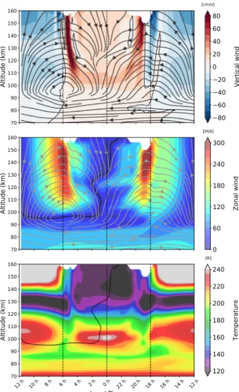
Fig. 1. (top) Vertical, (middle) absolute zonal wind speeds, and (bottom) temperature

at the equator averaged for one Vd. Streamlines show the circulation in the altitude vs. local time plan constructed from the average wind field shown in the top and middle panels. Thick solid line indicates where zonal wind values are zero.

Navarro et al., 2018) or other GCMs at a higher (Ando et al., 2016;

Takagi et al.,2018) or much higher (Kashimura et al.,2019) resolution, it is the highest resolution ever used for the upper atmosphere of Venus, compared for instance to 5◦ _× ₅◦ _in _{Brecht and Bougher} ₍₂₀₁₂_),

Brecht et al. (2021), or T21 (11.25◦ _{× 2.8125}◦_{) in} _{Hoshino et al.} (2012, 2013) and Nakagawa et al. (2013). Sugimoto et al. (2014) studied waves with the AFES GCM at a T63 (192 × 96) resolution and a model top at 120 km. However, their setup did not include any parameterization of upper atmospheric processes and they imple-mented a sponge layer starting at 80 km, thus efficiently damping atmospheric circulation in the upper atmosphere.Brecht and Bougher

(2012) deemed necessary an increased resolution in order to resolve the sharp horizontal temperature gradients near the terminators, and indeed resulted in substantial changes in our simulations, as will be detailed below. The major hurdle in implementing such an increased resolution is the high numerical instability of the simulations, with instabilities leading to unrealistic temperatures within a few tens of hours near the AS point in the upper atmosphere. To overcome this issue, we first ran the IPSL Venus GCM during one solar Venus day (Vd) from a converged initial state of the lower atmosphere obtained after 300 Vd in Garate-Lopez and Lebonnois (2018), and simplified prescribed altitude and solar zenith angle dependent distributions for

Fig. 2. Same as Fig. 1, but for absolute meridional wind speeds along the noon-midnight meridians averaged for one Vd.

CO2, CO, O, and N2species above 90 km (Hedin et al.,1983). We thus obtained an initial state stable for the full interactive photochemical package, suggesting that the numerical instabilities may arise from feedback loops between the upper atmosphere heating rates, dynamic chemical species, and the non-converged circulation of the downward moving flow near the AS point. We then obtained, after 29 Vd, a converged simulation with constant 1 Vd-averaged SS–AS wind speeds, without prescribed chemical species.

Additionally, the IPSL Venus GCM uses a stochastic parameteriza-tion of non-orographic gravity waves (Lott et al.,2012). Gravity waves are assumed to be generated at the top of the convective cells, located at about 55 km on Venus, propagate upwards, and break in the upper atmosphere. These waves were found to impact the circulation of the upper atmosphere (Zalucha et al.,2013;Gilli et al.,2017). To correctly implement this parameterization with the increased resolution, we corrected the minimal horizontal wavenumber 𝑘_𝑚𝑖𝑛of individual waves: 𝑘∗_𝑚𝑖𝑛= 𝑚𝑎𝑥(𝑘𝑚𝑖𝑛,

𝜋

𝐴) (1)

with 𝐴 the surface area of the grid cell.

3. Average structure of the nightside circulation

3.1. Horizontal wind

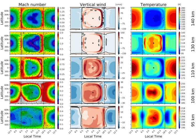
Atmospheric fields above 70 km and averaged for 1 Vd are shown as a function of local time inFig. 1, of latitude inFig. 2, and as maps

(5)

at different altitudes inFig. 3. The circulation is dominated by the SS– AS circulation above 100 km of altitude, with winds converging from the SS point to the AS point, and wind speed exceeding 300 m s−1_at the terminator. The RZS circulation is dominant below 85 km (Fig. 1), with values around 100 m s−1 _{at the cloud top (∼ 70 km). Between} 90 and 105 km approximately lies a transition region consisting of a reversal of the zonal wind from retrograde (westwards) to prograde (eastwards) values between local times 0 h and 12 h (Fig. 1).Figs. 1

and3also show an asymmetry of the SS–AS zonal flow between the morning and evening branches and between 120 and 130 km due to the breaking of non-orographic gravity waves at those altitudes (see companion paper). The wind is slightly more westwards on the average, with convergence shifted away between midnight and 2 h between about 100 and 130 km, as apparent in the zero zonal wind contour ofFig. 1. Conversely, the SS–AS meridional flow is symmetric between the Northern and Southern hemispheres (Fig. 2), as the non-orographic gravity waves’ drag is weaker on the meridional direction compared to the zonal one. Because of this structure, a point with null wind speed (both zonal and vertical) exists at the equator at local time 6 h, and between altitudes 95 to 100 km (see average equatorial wind streamlines inFig. 1).

3.2. Temperature

Temperature decreases with altitude until the transition region, where local maxima of 240 K are centered near the Sub-Solar (SS) and AS point (bottom panels ofFigs. 1and2). The warming at the SS point between altitudes 100 and 110 km is due to near-IR heating produced by CO2molecules non-LTE absorption of solar radiation, as pointed out byGilli et al.(2017) andBrecht and Bougher(2012) and observed by the VIRTIS instrument on board VEx (Gilli et al.,2015). The warming near the AS point has also been observed with VEx (Bertaux et al.,

2007;Piccialli et al.,2015) and is due to the downward flow of day-to-night air by adiabatic compression and advection from the dayside, as shown by Gilli et al.(2017) andBrecht and Bougher(2012). Above these warm layers, temperature decreases anew with altitude, until EUV heating warms the dayside above 140 km. The cold nightside temperatures above 120 km and below 140 km observed by Pioneer Venus (Schubert et al., 1980) are due to CO2 cooling at 15 μm (Gilli

et al., 2017). The terminators are cooler than other local times at altitudes 95 to 115 km as shown in Figs. 1, 2, and3. This result is not in agreement with Piccialli et al.(2017), probably because they used a-priori CO profiles fromClancy et al.(2012) up to 100 km, and a constant value above, whereas our model predicts instead CO volume mixing ratio decreasing above that altitude (see companion paperGilli et al.,2021). A more detailed comparison of the temperature structure of this simulation is given inGilli et al.(2021).

3.3. Shock-like feature and downward motion near the terminator These results are in general agreement with previously published GCM studies and observations, and the mechanisms at stake understood to a large extent. However, our simulations reveal a particular structure consisting of downward vertical speeds maximal near the terminator on the nightside, with larger values near the morning terminator than the evening terminator, reaching 100 cm s−1_{above 120 km (see top panel} inFig. 1). This downward motion is associated with sharp horizontal gradients of horizontal winds (Figs. 1, 2, and 3), with a decrease reaching up to 200 m s−1_{over a distance of 500 km and less. A local} increase of temperature of up to 40 K is also associated with this downward motion (Figs. 1,2,3and4), producing a nightside ‘‘hot ring’’ feature above 120 km, well visible in the time-averaged field at 130 km inFig. 3, or in the instantaneous field at 120 km inFig. 8.

The nature of this structure is not straightforward. It is reminis-cent of the ‘‘tongue’’ of downward vertical motion and local heating

simulated byDickinson and Ridley(1975,1977) with a 2D altitude-solar zenith angle model, orBougher et al.(1986) with a 3D GCM. The tongue-like shape is apparent in the vertical, horizontal winds and temperature fields inFigs. 1and2, with the structure moving away from the terminator towards the AS point as it gets lower in altitude. According toDickinson and Ridley(1975), the cause of the hot ring is adiabatic heating from the downward motion caused by the decrease in altitude of isobars past the terminator.

However, there is a major difference between our simulation and these past works. In our simulation, the horizontal wind speed is higher, with values greater than 300 m s−1_{at an altitude of 130 km, compared} to 250 m s−1 _in _{Dickinson and Ridley}₍₁₉₇₅_, ₁₉₇₇_{), and 200 m s}−1 inBougher et al.(1986). Our result is in agreement with more recent ground-based measurements of Doppler winds as high as 348 m s−1_on the morning terminator (Clancy et al.,2015). Therefore, the simulated winds are supersonic, with Mach numbers attaining a value of 2 at 130 km (Fig. 3), with the Mach number defined as 𝑀 = 𝑣∕𝑐𝑠 with 𝑣 the wind speed, the speed of sound 𝑐𝑠 =

√

𝛾𝑅𝑇∕, 𝛾 the heat capacity ratio, 𝑇 the temperature, 𝑅 the ideal gas constant, and the molar mass. Given the Mach number is well above unity in our sim-ulation, followed by a sharp wind decrease and temperature increase at altitudes above 120 km (Fig. 4), it is reasonable to investigate the presence of a supersonic shock wave as a possible cause of the structure in the vicinity of the terminator. Atmospheric supersonic shocks have been studied in the context of hot, highly irradiated, giant exoplanets (e.g.Rauscher and Menou,2010;Heng,2012), but quite rarely for the Venusian upper atmosphere. By considering the air densities measured by Pioneer Venus, Seiff(1982) briefly discussed the possibility of a shock in the Venusian upper atmosphere as a dissipation mechanism to slow down the SS–AS flow. Moreover,Clancy et al.(2015) estimated a Mach number 1.5 from their observations, andHoshino et al.(2012) simulated supersonic winds, but neither mentioned a shock.

The primitive equations of the IPSL dynamical core are based on the hydrostatic equilibrium. Therefore, vertically propagating sound waves are filtered out, leaving horizontally propagating sound waves, also known as Lamb waves (Vallis,2006, Chapter 2). Although the IPSL dynamical core can simulate Lamb waves because it is a compressible core, a standing Lamb wave steepening into a shock may not be properly simulated because of the large grid resolution (> 100 km) compared to the rapid changes of atmospheric variables over a small distance, typical of a shock.

The limitation of this GCM configuration does not preclude inves-tigating the possibility of a shock in the Venusian upper atmosphere. With a hydrostatic dynamical core having the same limitations, Show-man et al. (2009) reported a structure of strong convergence and temperature increase on a narrow region for a hot Jupiter at 1 mbar, while Rauscher and Menou(2010) discussed the nature of a similar feature and concluded it may be a Lamb wave. Drawing on this re-sult,Fromang et al. (2016) performed simulations using a dynamical core with a proper treatment for shocks, eventually showing that hot Jupiter were prone to shocks. This useful result is pertinent for our case, as it proves that features such as Lamb waves with a limited dynamical core can be the first clue that shocks may be simulated, and actually exist, in the Venusian upper atmosphere. Future dedicated studies may be tackled with a more suitable numerical code, for instance a finite-volume one, with a higher resolution near the terminator.

One way to detect shock-like features in a numerical code is to consider the variable 𝜂 = −𝛥𝑥∇⋅ 𝐯

𝑐_𝑠 , with 𝛥𝑥 the horizontal grid spac-ing.Zhu et al.(2013) andFromang et al.(2016) empirically identified shocks wherever 𝜂 has values greater than 0.2. In our simulation, we find 𝜂 to be smaller than 0.2 in the upper atmosphere, except at the hot ring location, with values of 𝜂 between 0.5 and 1. This fact alone strongly suggests a shock-like mechanism.

Another indication of a possible shock-like feature is the dependence of the SS–AS flow results on the horizontal resolution.Fig. 4provides

(6)

Fig. 3. Maps of Mach number, winds and temperature averaged for one Vd at 5 different altitudes. Black contour can indicate Mach number unity (left column) and zero vertical

wind speed (middle column). Positive values of vertical speeds indicate downward winds.

an example of equatorial Mach number and temperature at 130 km for two resolutions: high (the present study) and low (the same employed in Gilli et al.,2017). While horizontal supersonic speeds (𝑀 >1) are obtained for both resolutions, the decrease of 𝑀 below unity hap-pens rather abruptly for the high resolution, over just two grid points past the morning and evening terminators. In contrast, the transition from supersonic to subsonic flow occurs smoothly over thousands of kilometers with the low resolution. Moreover, temperature increases just after the decrease of 𝑀 for the high resolution, forming the ‘‘hot ring’’ feature described above, whereas no such local maximum of temperature happens for the low resolution simulation. This behavior of Mach number and temperature is in line with a shock-like feature: a decrease of 𝑀 past the feature, and an increase of temperature. Shocks, including Lamb waves, happen when regions of lower density (e.g. generated by a wave) acoustically propagate faster than regions of higher density, possibly converging together if the flow is supersonic, and forming a shock. The formation and location of the shock thus depends on the profile of density perturbations and the flow’s speed, temperature, and pressure along a streamline. Therefore, it makes sense that an increase in resolution is more suited to resolve the convergence of density perturbations and that a shock is eventually simulated as the resolution increases, as noted byFromang et al.(2016) in the context of hot Jupiters.

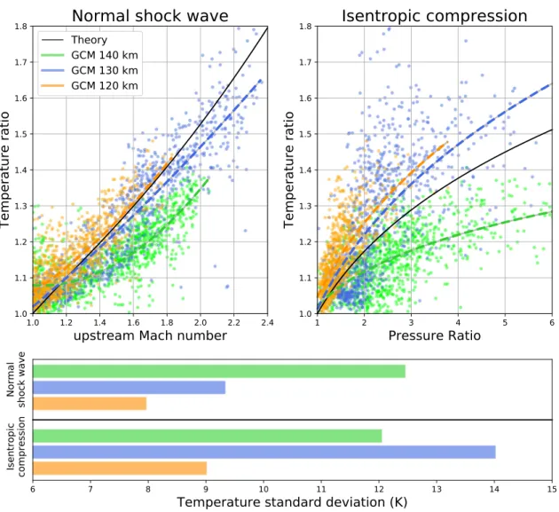
In order to test the hypothesis of a shock-like feature against sim-ulated values of temperatures and Mach number, we use the classic relation between temperature and Mach number of normal shock equa-tions from one-dimensional gas dynamics theory (e.g. Liepmann and Roshko,2001): 𝑇2 𝑇1 = ( 2𝛾𝑀2 1− (𝛾 − 1) ) ( (𝛾 − 1)𝑀2 1+ 2 ) (𝛾 + 1)2_𝑀2 1 (2) with subscripts 1 and 2 denoting the quantities upstream and down-stream of the shock-like feature, respectively. In this case, the increase

of temperature is a non-isentropic, irreversible, process caused by a decrease of wind speed. Alternatively, if the temperature increase were caused by adiabatic heating of descending air as found byDickinson and Ridley(1975,1977), the temperature ratio would be given by the isentropic relation: 𝑇2 𝑇₁ = (_𝑃 2 𝑃₁ )𝛾− 1 𝛾 (3) with 𝑃 the pressure.Fig. 5compares the temperature ratio of the hot ring to Eqs.(2)and(3). At altitudes of 120 and 130 km, the general trend of the temperature increase in the hot ring is in broad agreement with a shock-like feature as given by Eq.(2). At an altitude of 140 km, the temperature increase is, in general, systematically smaller by 20% than the one expected for a shock. Isentropic compression alone does not seem to account for the simulated increase in temperature, espe-cially at a high pressure ratio. The standard deviation between expected and simulated temperatures is smaller at 120 and 130 km for the case of a normal shock than for an isentropic compression (Fig. 5).

All in all, these results suggest that a strong (i.e. with 𝑀 > 1 upstream and 𝑀 < 1 downstream), normal, shock-like feature in the form a of standing Lamb wave, is present in our simulations above 120 km and is the main reason for the hot ring and strong wind deceleration. The enhanced downward motion must also play a role and will inevitably warm the descending air by adiabatic compression, but it is not the chief reason for the hot ring and wind deceleration above 120 km. Between 110 km and 120 km, where wind speeds are subsonic, adiabatic warming would then be the main reason for the persisting hot ring at those lower altitudes. Other processes also play a role, such as near-IR heating that may be responsible for slightly higher than expected temperature ratios at 120 km, and thermal conduction, possibly responsible for the lower than expected ones at 140 km. Moreover, and as pointed out by Seiff (1982), the air needs to be

(7)

Fig. 4. Equatorial Mach number and temperature at an altitude of 130 km for high (96 × 96) and low (48 × 32) resolutions. The atmospheric flow is directed towards the AS

point at local time 0 h. Dots indicate the horizontal spacing for each model resolution.

diabatically cooled to avoid high unrealistic nightside temperatures regardless of the cause of the hot ring.

It results that there is a normal shock-like feature, dissipating kinetic energy, resulting in downstream increased temperature, pressure, and density. The shock-like feature is the strongest at an altitude of 130 km, with 𝑀 ∼ 2 (Fig. 3). The horizontal wind speed upstream of the shock-like feature increases roughly from 200 m s−1_{at 110 km to 300 m s}−1 at 130 km (Figs. 1and2), while the upstream temperature roughly decreases from 200 K at 110 km to 100 K at 130 km, and then increases to 200 K at 140 km in the thermosphere. Therefore, as 𝑀 ∝ _√‖𝐯‖

𝑇 , the largest impact on the Mach number upstream of the shock-like feature is the local minimum of temperature with altitude, located at 130 km. This structure consisting of a shock-like feature above ∼ 120 km, and adiabatic heating below, would be apparent in the temperature and density structures of horizontal profiles, but so far no such observation seems to exist. The nightside temperature maps measured by SPICAV on board VEx (Piccialli et al.,2015) are scattered, and their coverage is quite limited at the local times of the terminator structure, at 18–20 h and 4–6 h.Piccialli et al.(2015, figure 7) show a 15 K bump centered at 19 h at 115 km, but is much less than the variability of the nightside, as explained in the next section. Moreover,Clancy et al.(2015) retrieved supersonic cross-terminator zonal winds at 100 to 125 km, with faster winds in the evening than in the morning side, which is the case in our simulation at altitudes 130 km and above (Fig. 1).

4. Variability of the nightside dynamics

The time-averaged view of atmospheric fields in Section3does not show a crucial point of the GCM results: the strong variability of the nightside, in stark contrast to the quiet dayside, as seen inFigs. 6,7, and

8. The SS–AS circulation on the dayside is very simply described as a time-independent increase of horizontal winds with solar zenith angle, modest temperature changes of less than 10 K at any location, and an almost constant atmospheric composition of 96% CO₂. Meanwhile, the nightside is subject to abrupt changes of atmospheric composition, horizontal wind velocity, vertical wind speed, and temperature on a timescale of tens of hours.

As SS–AS horizontal winds are decreased due to non-orographic gravity waves, a shock-like feature, and downward motion at the ter-minator, converging air flows form multiple local subsiding ∼ 1000 km size eddies that vary in strength and location in a seemingly unstruc-tured way. This behavior is apparent in the local maxima and minima of wind vorticity (e.g. at 130 km in Fig. 7), with those eddies on the nightside forming and disappearing in a matter of a few hours. The changes of horizontal wind speed induce a change in atmospheric composition. Indeed, CO2 is photodissociated into O and CO on the dayside, and air depleted in CO2 piles up wherever horizontal wind gets slower. CO2 concentration thus varies in both local time and latitude (Fig. 6). Moreover, individual species start to diffuse separately according to their masses above the homopause due to molecular diffusion, leading to the prevalence of the lightest species, such as CO and O. Therefore, air composition is a tracer of dynamics on the

(8)

Fig. 5. Top: ‘‘Hot ring’’ temperature ratio as a function of upstream Mach number and pressure ratio. Black solid lines indicate the analytical 1-D normal shock equation given

by Eq.(2)or the isentropic compression by Eq.(3). Dots indicate GCM values, and dashed color lines indicate the best fit to those values. Bottom: standard deviation between the GCM simulated temperature and Eqs.(2)and(3)for each case. The downstream (upstream) values are obtained for 10 Earth days from the locations of the local maximum (minimum) of temperature after (before) 𝑀 − 1 become negative along the SS–AS lines. (For interpretation of the references to color in this figure legend, the reader is referred to the web version of this article.)

nightside, with air composition and wind speed well correlated in

Fig. 6. The varying vertical wind speed is well correlated locally with nightside temperatures, as the descending air is warmed by adiabatic compression in the region between the AS point and the hot ring caused by the shock-like feature (Fig. 8).

Such behavior of highly time-variable planetary scale structures on the nightside is not seen in simulations at lower resolution with the same GCM (Gilli et al., 2017), and was not reported with other GCMs (Brecht et al., 2011; Hoshino et al., 2012; Nakagawa et al.,

2013), all having a lower resolution than the GCM simulation presented here. Fig. 9 compares the time-integrated eddy enstrophy 𝑞 on the daysides and nightsides of simulations at low (7.5◦_{× 5.625}◦_{) and high} (3.75◦_{× 1.875}◦_{) resolution with:}

𝑞(𝑧) =

∫𝐷|∇ × 𝐔|

2

𝑑𝑆 (4)

with z the altitude and D the considered domain (e.g nightside or dayside). Eddy enstrophy is a useful quantity to assess eddy activity and the transience of the atmospheric flow. It gives a global metric of the wind vorticity and the associated energy per mass. The difference of eddy enstrophy by a factor 5 inFig. 9at altitudes 70 to 85 km between the two GCM resolutions is simply due to increased resolution that resolves more eddies. For the high resolution, eddy enstrophy above 90 km is seven times higher on the nightside than on the dayside.

The difference between dayside and nightside eddy enstrophy increases to a factor 10 at 100 km for both resolutions, with a smaller spread, because the circulation of the dayside flow is direct and less variable than on the nightside. Above 110 km, the nightside enstrophy at high resolution does not vary much with altitude, whereas the low resolution one decreases by a factor around 3 between 110 and 130 km. The reason for such a difference between the two different resolutions is the presence of the shock-like feature above 110 km in the high-resolution case only, which reduces horizontal wind speeds and increases the number of large-scale eddies downstream of this shock-like feature. It is worth noting that eddy enstrophy is nearly constant with altitude above 100 km, so potential vorticity is not conserved, indicating a sink or source of potential vorticity from diabatic heating in the upper at-mosphere, unlike the polar vortex at the cloud deck level (Garate-Lopez and Lebonnois,2018).

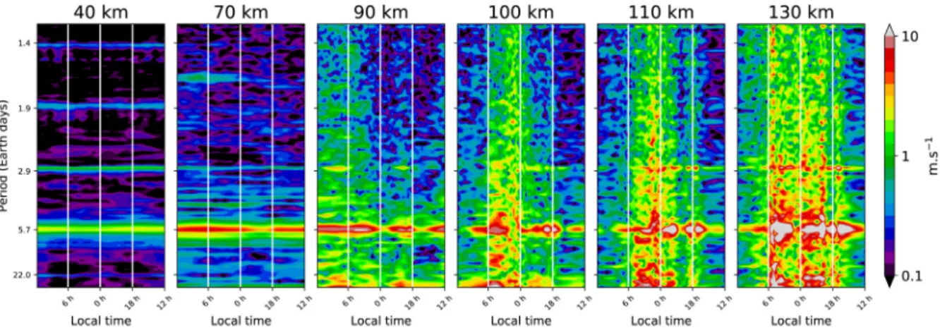
Fig. 10presents the periodograms of equatorial wind speed as a function of altitude and local time. There is a dominant 5.7 Earth days period at all altitudes above 40 km due to a Kelvin wave, as further explained in Section5. Another period at 2.9 Earth days is also present at all those altitudes. The periodicity does not depend on local time in the lower atmosphere, in contrast with the transition and SS–AS regions. At 90 km, in the transition region, the atmospheric flow is more variable from midnight to noon, that is to say downstream to the AS

(9)

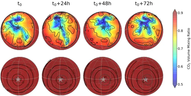
Fig. 6. Snapshots 24 h apart each of (colors) CO2in volume mixing ratio and (contour) wind speed in m s−1at an altitude of 130 km for the (top) nightside and (bottom) dayside

of Venus. The position of the subsolar point is indicated by a light gray star and the antisolar point by a dark gray star. (For interpretation of the references to color in this figure legend, the reader is referred to the web version of this article.)

Fig. 7. Same asFig. 6with (colors) wind vorticity and wind streamlines at an altitude of 130 km for the (top) nightside and (bottom) dayside of Venus. (For interpretation of the references to color in this figure legend, the reader is referred to the web version of this article.)

point and below the inversion of zonal wind at the morning terminator (Figs. 1and3), than from noon to midnight, upstream of the AS point. Above 100 km, the local times for which the wind variability is greater are found between 0 h and 6 h. At 130 km, the whole nightside is variable, in contrast to a quieter dayside. The impact of the shock-like feature on wind variability is obvious at 130 km, with higher nightside variability clearly delimited at the location of the shock-like feature near the terminators. The 5.7-day period caused by the Kelvin wave is a major periodicity for all the atmospheric layers, but we could not assess if smaller frequencies would exist without it. In other words, it is not clear if the strong variability of the equatorial horizontal wind at high altitudes, and by extension of the upper atmosphere in general, requires this 5.7-day period from the lower atmosphere, or if it is an inherent characteristic of the nightside dynamics caused by the shock-like feature and downward motion.

5. Impact of the Kelvin wave

Kelvin waves in the Venusian atmosphere have been observed (e.g. Belton et al. (1976), Covey and Schubert (1982), del Genio and Rossow(1990)) and modeled (e.g.Yamamoto,2019) on multiple occasions. Our simulation produces a westward propagating Kelvin wave excited in the middle and upper cloud deck, between 60 and 65 km. This Kelvin wave appears when a sufficiently strong zonal wind produces a Coriolis force for the local atmospheric flow (Peralta et al.,

2015). The Kelvin wave may be linked to the meridional discontinuity observed in the lower cloud (Peralta et al.,2020). The detailed char-acteristics of this wave in the lower atmosphere are beyond the scope of this paper, but we can nevertheless briefly mention its main points. This wave also enters in resonance with a Rossby mode at mid-latitudes, forming a Kelvin–Rossby instability (Wang and Mitchell,2014). Note

(10)

Fig. 8. Same asFig. 6with (colors) temperature and (contours) vertical wind speed (cm/s, downward positive) at an altitude of 120 km for the (top) nightside and (bottom) dayside of Venus. (For interpretation of the references to color in this figure legend, the reader is referred to the web version of this article.)

Fig. 9. Eddy enstrophy as a function of altitude averaged over 1 Vd and latitude lower

than 75◦_{, on the day and night sides, at high (96 × 96) and low (48 × 32) resolutions.}

The envelopes show the minima and maxima for 1 Vd.

that under Venusian conditions, and as it spans more than 100 km in altitude, the true nature of the wave we simulate is not straightforward, and may be a Kelvin-like, a Kelvin–Rossby type, or else. Therefore, we simply refer to it as a ‘‘Kelvin wave‘‘ and leave those considerations for further studies. When it reaches the cloud top, we note that the Kelvin

wave has an average zonal wind amplitude of 5 m s−1 _{at 70 km and} 15 m s−1_{at 80 km (}_{Fig. 11}_{), and its latitudinal extent is 60}◦_{S to 60}◦_N. The period of this wave is 5.7 Earth days (Fig. 10) and depends on the zonal wind speed below the cloud deck. At the cloud top, this wave propagates slower than the mean zonal wind, while recent Akatsuki UV observations suggest that the Kelvin wave propagates faster (Imai et al.,

2020). As our GCM underestimates the zonal wind speed at altitudes 30 to 40 km (Garate-Lopez and Lebonnois,2018, Fig. 5), we would expect the period of the wave to be actually lower (Peralta et al.,2020). All in all, our simulated Kelvin wave’s period and amplitude are in general agreement with observations of the cloud top (Imai et al.,2016;Imai et al.,2020), even if its period is too large, and if the morphology of the Y-feature is not apparent in the simulated zonal wind field at a fixed altitude or pressure. The absence of this feature could be due to the lack of a transported UV absorber in the GCM, that reveals such a spatial pattern in the observations (Peralta et al.,2015).

5.1. Impact on the upper atmosphere

The Kelvin wave has a considerable impact on both the transition region and the SS–AS circulation. The phase and amplitude structure of the equatorial zonal wind perturbed by the Kelvin wave is shown in

Fig. 11. The wave has a wavenumber-1 structure up to roughly 95 km, and perturbs the wind field above and excites wind fluctuations that are seen with high amplitude on the nightside, but much less on the dayside (though they are still present). These fluctuations are excited by the wavenumber-1 Kelvin wave below 95 km, but do not keep this wavenumber-1 structure as they do not propagate upward the same way in the night and in the day. These perturbations are certainly secondary waves, excited by the Kelvin equatorial wave.

Therefore, the Kelvin wave is able to impact the SS–AS circulation except for local times close to noon. This result is contrary to the conclusion of analytical models, using idealized zonal wind vertical profiles of decreasing speed above the cloud top (Kouyama et al.,2015;

Nara et al., 2020), that a Kelvin wave is attenuated below 80 km. Indeed, the structure of the zonal wind simulated by the IPSL VGCM is different, with speeds higher than 100 m s−1 _{on average in the} transition region at the vicinity of the evening terminator (Fig. 1).

Brecht et al.(2021) prescribed Kelvin and Rossby waves-like per-turbations in an upper atmosphere GCM with a lower boundary at 70 km, and found that the Kelvin wave propagate up to 110 km

(11)

Fig. 10. Periodograms of equatorial (10◦_S-10◦_{N) horizontal wind speed at different altitudes.}

Fig. 11. Spectral decomposition of equatorial (10◦_S-10◦_{N) zonal wind at frequency 2𝜋/T, with T = 5.7 Earth days, showing the westwards propagation and impact of the Kelvin}

wave for half of its period. The cloud bottom and top altitudes are indicated at 48 and 70 km. Thick solid line indicates where zonal wind values are zero on average. Upper and lower limits of the cloud deck are represented by two horizontal gray lines. The time zero is chosen as the cloud top maximum at local time 12 h.

only, due to differences with their vertical wind profile and amplitude and wavelength of their wave forcing, compared to the Kelvin wave naturally simulated in the IPSL GCM.

As a consequence of the resulting vertical profiles of horizontal wind, the zonal wind field impacted by the Kelvin wave inFig. 11is a complex structure, and is not straightforward to interpret. The vertical wavelength is 15 km in the lower and middle cloud deck, with an amplitude of 10 m s−1₍_{Peralta et al.}_,₂₀₂₀_{). In the upper cloud deck,} the vertical wavelength dramatically changes, and is equal to 50 km, comparable to Hoshino et al. (2012). Downstream of the shock-like feature and downward motion on the nightside terminator, the zonal wind is 180◦ _{out-of-phase with the upstream side. This makes sense} because in case of a shock, the faster a supersonic flow is, the slower the downstream subsonic flow is (c.f. Liepmann and Roshko,2001). Another contribution to the out-of-phase structure on the nightside is the retrograde zonal flow entering from the transition region inside the region delimited by the shock-like feature, creating a temporary reversal of the SS–AS flow at 110 km with a delay of a few tens of hours. This reversal can be seen in the meridional wind structure of

Fig. 12.

5.2. Impact on the nightside transition region

Fig. 12 shows the impact of the Kelvin wave on the meridional wind and oxygen species as the wave passes through the night. In the absence of a Kelvin wave, the SS–AS winds at 110 km are balanced in all directions, creating a convergence at the AS point. The Kelvin wave perturbs the zonal wind in the transition region below 95 km,

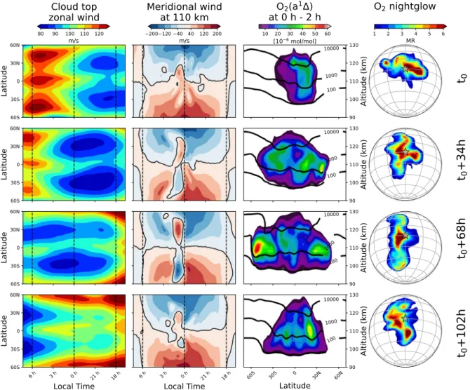
creating a retrograde imbalance of the flow towards the morning side. As westwards wind rushes into the nightside from the evening terminator, two 2000 km large-scale transient vortices are formed in the transition region between local times midnight and 3 h, one in each hemisphere, as also seen inFig. 15. As a consequence, a strong poleward transport attaining 150 m s−1 _{is present for approximately} 100 h in both hemispheres, up to 60◦_{latitude and 130 km of altitude.} This causes the periodic transport of atomic oxygen to high latitudes after its downward transport. The location of the recombination of oxygen into O₂(1_𝛥_{) thus happens at all latitudes from the equator to 60}◦ in the transition region, with periodic episodes of high latitude 1.27 μm oxygen nightglow (Fig. 14).

5.3. Impact on the dayside SS-AS circulation

Similarly,Fig. 13shows the impact of the Kelvin wave on the circu-lation and O species at 130 km of altitude. At this altitude, the Kelvin wave has a negligible impact on the zonal wind between local times 6 h and 15 h. Between 15 h and 18 h, the Kelvin wave creates a local maximum (minimum) of horizontal wind lasting approximately 100 h when the Kelvin wave cloud top zonal wind is minimum (maximum). This is shown in the panel at times 0 and 3T/8 ofFig. 11, with zonal wind maximum on the nightside in the RZS circulation, ducting into the dayside of the SS–AS circulation from the evening terminator. Then, the whole nightside is impacted by the Kelvin wave perturbation on the SS–AS evening branch, even if the Kelvin wave does not propagate into in the SS–AS morning branch between local times midnight to noon due to the zonal wind inversion at altitude 95 km. Since the cloud top zonal

(12)

Fig. 12. Four consecutive snapshots, from left to right, of: (1) map of cloud top zonal wind, (2) map of meridional wind at 110 km, (3) latitude vs. altitude volume mixing ratio

of O2(1𝛥𝑔) (colors) and O (contours), (4) O2nightglow at 1.27 μm, with the AS point indicated by a gray star. (For interpretation of the references to color in this figure legend,

the reader is referred to the web version of this article.)

Fig. 13. Left: Equatorial zonal wind at 70 km (black contours) and 130 km (colors). Right: Column density of atomic oxygen for altitudes above 130 km (colors). Gray shaded

areas indicate where the vertical wind is greater than 17 cm s−1_{upwards at an altitude of 130 km. (For interpretation of the references to color in this figure legend, the reader}

(13)

Fig. 14. Time series of noon cloud top zonal wind speed, dayside O column abundance above 130 km as a proxy for OI 135.6 nm dayglow, and O2nightglow at 1.27 μm at mid

latitudes.

wind is maximum, the dayside SS–AS circulation is weakened, and thus the dayside upwards vertical wind is decreased (Fig. 13). Conversely, the upwards vertical wind is increased when the cloud top zonal wind is minimum. As can be seen in the right panel ofFig. 13, this increase of upwards motion, associated with a decrease of horizontal wind between 15 h and 18 h, favors a decrease of CO₂abundance above 130 km, and an increase of O and CO abundances. Indeed, as explained in Section3, the air composition at altitudes where CO2 is being photodissociated depends on the local wind speeds. For instance, the vertically integrated column of O above 130 km, shown in Fig. 13, increases from 20 to 25 moles km−2_{. All in all, CO}

2varies by 2000 ppm on the dayside due to the Kelvin wave, much less than the difference between the dayside and the nightside.

6. Oxygen airglows

The structure of the upper atmosphere and the impact of the Kelvin wave help us to understand the observations of two airglows: the emis-sion of O2(1𝛥) at 1.27 μm, and OI at 135.6 nm. We focus on these two airglows because they notably reveal the circulation at different local times and altitudes. Our GCM simulation provides new insights into the existing observations of these airglows. Other emissions have been observed, such as the nitric oxide UV nightglow (Stewart et al.,1980;

Stiepen et al., 2013), OII 83.4 nm and OI 130.4 nm dayglows ( Ma-sunaga et al.,2015,2017). However, the IPSL GCM does not yet include the nitrogen chemistry, and the OI emission at 130.4 nm is optically thick, making it difficult to interpret the O abundance (Masunaga et al.,

2015).

6.1. O₂(1_{𝛥) nightglow}

While O, O2, and CO2 are dynamical tracers computed online in the IPSL Venus GCM, the O₂(1_𝛥_{) nightglow at 1.27 μm can be entirely} calculated offline from the simulated GCM atmospheric fields. We employ the reaction rate coefficient 𝑘1 of the trimolecular reaction O + O + CO2→O2(1𝛥) + CO2 given byCampbell and Gray(1973):

𝑘₁= 2.5 × 9.4610−34exp(485 𝑇

)

(5) with 𝑇 the temperature. The volume emission rate VER (in photons.cm−3_s−1_{= 10}−4_{kR km}−1_{) is calculated as:}

VER = 𝜖𝑘1 𝑛_𝑐𝑜 2𝑛 2 𝑜 1 + 𝜏𝑞𝑛_𝑐𝑜 2 (6) with 𝑛𝑐𝑜2 and 𝑛𝑜 the concentration of CO2 and O species in

molecules.cm−3, 𝜏 = 4470 s the Einstein coefficient, a quenching coefficient 𝑞 = 0.5 × 10−20 _cm3 _molecule−1_s−1_{, and 𝜖 the fraction of} molecules produced in the O2(1𝛥)state, rather than in higher excited

states. This fraction is quite uncertain and may lie between 0.6 and 1. In his detailed discussion,Krasnopolsky(2011) recommended a value of 0.7. We adopted 𝜖 = 0.75 for consistency withGérard et al.(2009) andSoret et al.(2012). In this paper we present the nightside column integrated O2(1𝛥) nightglow (Figs. 12,15, and Appendix A), as it would be observed from nadir (Crisp et al.,1996;Lellouch et al.,1997;Hueso et al.,2008;Soret et al.,2012,2014;Gorinov et al.,2018). On average, the nightglow is centered on the AS point. Still, the strong variability, detailed previously in Sections4and5, creates a varied morphology of the nightglow’s spatial structure. Nightglow intensity varies up to 12 MR in the vicinity of the AS point. Elongated structures up to 8 MR at mid-latitudes (30◦_{to 60}◦_{) seen by}_{Crisp et al.}₍₁₉₉₆_{) and}_{Soret et al.} (2014) are large-scale fronts created by the periodic poleward transport in the transition region triggered by the Kelvin wave, and associated with a 2000 km size vortex that varies on a daily timescale, as seen byGérard et al.(2014). At lower latitudes, below 30◦_{, highly variable} bright spots are caused by eddies of subsiding flow whose location and intensity vary on a 10 h timescale.

6.2. OI 135.6 nm dayglow

OI 135.6 nm emission dayglow is produced by photoelectron impact in the upper atmosphere and is nearly proportional to O column density above 130 km (Masunaga et al., 2015; Nakamura et al., 2016). As explained in Section5, the amount of atomic oxygen on the dayside is periodic and in phase with the cloud top noon zonal wind.Fig. 14

shows the time series of zonal wind and O dayside column as a proxy for the OI 135.6 nm dayglow. The total amount of dayside O is approximately 35 × 1028_{moles above 130 km, with variations ranging} from 2 × 1028_{to 3 × 10}28_{moles, giving a variation of ∼6 to ∼8%. This} value compares well to the ∼4% variation of dayglow reported byNara et al. (2020). The difference in observed and simulated variations may be explained by the fact that these observations were restricted to the morning side, and that the proportionality between O density and dayglow is sensitive to UV solar intensity. At the same time, we integrate the whole dayside with an average solar intensity in the GCM.Nara et al. (2020) reported a 3.6-day periodicity in both the dayglow and the cloud top zonal wind andMasunaga et al. (2015) a 4-day periodicity, while our model simulates a 5.7-day periodicity. This discrepancy stems from the atmospheric dynamics in the deep atmosphere in the cloud deck, since the Kelvin wave originates, as explained in Section5. Artificially imposing more realistic faster winds in this region in the GCM results in a faster phase speed of the Kelvin wave (Peralta et al.,2020), as the Kelvin wave phase velocity depends on the zonal wind vertical profile (Peralta et al.,2015).

(14)

Fig. 15. 1.27 μm oxygen nightglow with wind arrows at 95 km. The black contours indicate the cloud top zonal retrograde wind at 100 m s−1_{to show how the wind field is}

perturbed by the Kelvin wave underneath. See Appendix A for an animated version of this figure. (For interpretation of the references to color in this figure legend, the reader is referred to the web version of this article.)

6.3. Airglow intensities and cloud deck dynamics

Nara et al.(2020) reported and modeled a phase lag of 4 ± 2 h between the noon cloud top and the O dayglow intensity, and explained it as the sum of the times of vertical propagation of waves and diffusion of O. The mechanism revealed by our simulation does not let us determine on a phase lag. The complex pattern of wave propagation in the thermosphere (Fig. 11) is not entirely understood, while the analysis of simulated time series of zonal wind and O density suggest the absence of a phase lag between the noon cloud top and the O dayglow intensity (Fig. 14). The phase lag in the observations could be an artifact caused by uncertainties to the sensing altitude at the cloud top, and noise and sampling. Alternatively, the IPSL Venus GCM in its present form could inaccurately estimate a zero phase lag, due to

inaccurate modeled background wind and temperature fields affecting the vertical propagation and impact of the Kelvin wave.

Interestingly, the same periodicity is also clearly visible in the O₂ nightglow emission at mid-latitudes, lagging behind the noon cloud top zonal maximum by approximately one-fourth of the Kelvin wave period, i.e. ∼1.4 days. This phase lag is due to the phase lag of the Kelvin wave structure between the cloud top at the SS point, and the transition region at the AS point and the transport of O enriched air to high latitudes from the equator to mid-latitudes. The former is approximately one-eighth of the Kelvin wave period, as can be seen in the panel T/8 ofFig. 11, i.e. ∼0.7 days. The latter corresponds to the transport of oxygen over from 30◦ _{to 50}◦ _{latitude at ∼80 m s}−1 (Fig. 12), i.e. ∼0.3 days. To our knowledge, no periodic behavior in the observations of the O2(1𝛥) nightglow has ever been reported.

(15)

Fig. 16. Relative contributions of horizontal transport, vertical transport, and chemical reactions in the apparent motion of O2nightglow. AG stands for AirGlow column emission.

7. Interpreting nightglow’s apparent motions

Hueso et al.(2008),Soret et al.(2014), andGorinov et al.(2018) tracked the observed O2 nightglow emission and derived its apparent horizontal motions. Variations of O₂ nightglow can be caused by hori-zontal transport, vertical transport, chemical reactions, or local change in temperature or density. Thus, the apparent motion is not necessarily equal to actual horizontal wind speeds, as hinted by Ohtsuki et al.

(2008), who pointed out the importance of local strong downward flows on the O2 nightglow. Therefore, how, when, and where the O2 nightglow apparent motion is a good tracer of the atmospheric flow is a legitimate question. Since we benefit from a GCM able to simulate reasonably well the O2nightglow emission, the first model capable of reproducing the variability and high latitude events of observations, we aim to address this question.

(16)

A first look atFig. 15and associated animation (see Appendix A) reveals that large scale eddies play an important role in the nightglow apparent motion. O₂(1_𝛥_{)-enriched air is trapped inside downwelling} eddies, and is every so often ejected from the eddy as it is disrupted or merges with other eddies. Those eddies are produced by the highly variable motion of flow past the shock-like feature in the thermosphere, and are subject to intense vertical downwards motion (Fig. 7), directly transporting atomic oxygen from higher altitudes, and eventually being a favored location of O2(1𝛥) production. This could explain the bright emission patches observed by Ohtsuki et al. (2008), and seen and tracked in Soret et al. (2014), implying that their apparent motions reflect the eddy motion, rather than horizontal winds. Emission at high latitudes are caused by the poleward transport of O. Since this transport stops after a few tens of hours, the apparent motion at the front of the elongated structure is caused by the progressive lack of O available for recombination. This may have been observed byGorinov et al.(2018), with elongated structures at high latitudes subject to a decrease of intensity at the end of the Kelvin wave cycle.

To quantify these behaviors, we computed the respective contribu-tions from three terms responsible for the nightglow apparent motion: namely horizontal transport, vertical transport, and chemical reactions. Other terms, such as diffusion, are orders of magnitude smaller than these three terms. The apparent motion is related to the local change of the volume emission rate VER computed in Eq.(6):

𝑑VER 𝑑t =

𝜕VER 𝜕t ||||chem

+ 𝐔⋅ ∇VER (7)

with 𝐔 the Eulerian wind. The chemical contribution is obtained from the recombination of atomic oxygen with rate coefficient 𝑘1 from Eq.(5)for the source term, with inverse lifetime of k2 = 1/𝜏 = 1/4470 s−1₍_{Lafferty et al.}_,₁₉₉₈_{) for the sink term:}

𝜕VER 𝜕t ||||chem

= 𝜖𝑘1𝑛𝑐𝑜2𝑛

2

𝑜− 𝑘2𝑛𝑜2(1𝛥)− 𝑞𝑛𝑜2(1𝛥)𝑛𝑐𝑜2 (8)

Thus, the horizontal, vertical, and chemical contributions to𝑑VER 𝑑t , respectively noted h, v, and c, are computed as:

ℎ=|𝑈𝑥𝑑𝑥VER + 𝑈𝑦𝑑𝑦VER| (9)

𝑣=_|𝑈𝑧𝑑𝑧VER| (10)

𝑐=|𝜖𝑘1𝑛𝑐𝑜2𝑛

2

𝑜− 𝑘2𝑛𝑜2(1𝛥)− 𝑞𝑛𝑐𝑜2𝑛𝑜2| (11)

with 𝑑𝑥, 𝑑𝑦, and 𝑑𝑧 the derivatives with respect to the x, y, and z directions. The ratios ℎ ℎ+ 𝑣 + 𝑐, 𝑣 ℎ+ 𝑣 + 𝑐, and 𝑐 ℎ+ 𝑣 + 𝑐, vertically weighted by VER, and averaged for four classes of total column intensity, are shown as maps in Fig. 16. On average, it is rare that one single contribution accounts for more than two-thirds of the total nightglow variation, meaning that, generally speaking, each of the three terms has comparable values. The vertical profiles for each contribution in

Fig. 16 show that where the VER peaks near 95 km, the chemical contribution accounts for 50% of the VER variation, the horizontal transport for 30%, and the vertical one for 20%. Indeed, this altitude in the transition region is the major location of O2(1𝛥) production and loss, while the nightside circulation is mostly horizontal. The vertical transport dominates the horizontal one above 100 km, with downward motion of the SS–AS circulation, and a peak of the relative abundance (volume mixing ratio) of O2(1𝛥) inFig. 12near 110 km, higher than the VER peak at 95 km.

For nightglow emission < 1 MR, vertical transport dominates be-tween local times 0 h and 22 h. At higher nightglow emissions, hori-zontal transport plays a dominant role. For nightglow emissions > 2 MR and more, the chemical contribution dominates at latitudes greater than 30◦_{, as it corresponds to episodes of strong changes driven by} the sudden influx or lack or atomic oxygen, such as the bright patches confined in eddies, or the high latitude episodes triggered by the Kelvin wave.

These results show that horizontal motions cannot alone explain the apparent motion of the fast changing nightglow in the complex circulation of the transition region, unlike clouds that act as mostly passive tracers, usually in quieter atmospheric flow. It does not mean that existing observations of nightglow apparent motion are necessarily poorly correlated with horizontal wind speeds. It rather means that apparent motion should be analyzed with caution, especially if such an analysis spans wide ranges of latitudes, local times, total emissions, morphology patterns, and Kelvin wave phases. For instance, manual tracking (Gorinov et al., 2018) discards features that are deformed or disappeared over short timescales, ensuring a crude, pragmatic, filtering that might select horizontal transport over vertical transport and chemical variations.

Interpreting nightglow apparent motion can greatly benefit from the outputs of such a GCM. Data assimilation would be an ideal technique for this feat, as it would optimally combine both the information given by observations and a GCM. It would be an interesting application to the emerging field of Venusian data assimilation (Sugimoto et al.,

2017). Moreover, it could serve for the identification of possible GCM biases in the transition region, which is sensitive to both upper and lower atmosphere processes.

8. Discussion

Though we provided clues to long-standing scientific questions per-taining to Venus upper atmospheric circulation, some open questions remain nevertheless. These questions may be answered with further GCM studies with an emphasis on comparison between models, includ-ing data assimilation, as well as the analysis of existinclud-ing observations and the planning of future ones:

8.1. Is there a supersonic shock in the Venusian upper atmosphere? We provided evidence that the ‘‘hot ring’’ may indicate a shock, but the limitations of the dynamical core of the IPSL GCM currently only hints, but does not prove, that a shock may develop in the flow of the SS–AS circulation. The fact that the vertical component of sound waves are filtered out by the hydrostatic dynamical core probably hinders the modelling of the three dimensional structure of the shock-like feature. For instance,Fromang et al. (2016) found that vertical shear instabilities were leading to weak shocks in hot Jupiters. A shock-resolving code, applied to Venus, will answer the question of if and how a shock can actually form in its upper atmosphere.

One piece of the puzzle might be the measurements of cross-terminator supersonic winds byClancy et al.(2015), showing a major unexplained characteristic: their high temporal variability, more than 100 m s−1 _{over an hourly timescale, with a fine limb resolution of} ∼0.2 h in local time, but a large horizontal resolution of 3000 km. They concluded that an unknown large-scale forcing mechanism must be invoked to account for these changes. Such a mechanism could be a moving shock, as it is a process that reduces wind speeds. Our simulations predict the Kelvin wave makes the shock-like feature position oscillate by ∼0.5 h in local time on the evening, and ∼0.2 h on the morning (left panel ofFig. 13). Thus, the measurements may have caught a shock passing through the limb, efficiently reducing wind velocity upstream.

8.2. What are the parameters controlling the characteristics of the Kelvin wave and the possible shock in the upper atmosphere?

The complex circulation modeled by the GCM creates waves that play a key role in atmospheric physical processes. However, under the complexity of the modeled waves (for instance the patterns ofFig. 11) and because of the lack of sufficient observational constraints, it not clear what controls some of their important characteristics, such as their amplitude, the location of the shock-like feature, the propagation