HAL Id: hal-01497681
https://hal.sorbonne-universite.fr/hal-01497681
Submitted on 29 Mar 2017
HAL is a multi-disciplinary open access
archive for the deposit and dissemination of
sci-entific research documents, whether they are
pub-lished or not. The documents may come from
teaching and research institutions in France or
abroad, or from public or private research centers.
L’archive ouverte pluridisciplinaire HAL, est
destinée au dépôt et à la diffusion de documents
scientifiques de niveau recherche, publiés ou non,
émanant des établissements d’enseignement et de
recherche français ou étrangers, des laboratoires
publics ou privés.
To cite this version:
Alizée Pottier, François Forget, Franck Montmessin, Thomas Navarro, Aymeric Spiga, et al..
Unrav-eling the Martian water cycle with high-resolution global climate simulations. Icarus, Elsevier, 2017,
291, pp.82-106. �10.1016/j.icarus.2017.02.016�. �hal-01497681�
ACCEPTED MANUSCRIPT
Unraveling the Martian water cycle with high-resolution global climate
simulations
Aliz´ee Pottiera,b,∗, Fran¸cois Forgetb, Franck Montmessina, Thomas Navarrob, Aymeric Spigab, Ehouarn
Millourb, Andr´e Szantaib, Jean-Baptiste Madeleineb
aLATMOS/IPSL, UPMC Univ. Paris 06 Sorbonne Universit´es, UVSQ, CNRS, Guyancourt, France bLaboratoire de M´et´eorologie Dynamique/IPSL/CNRS, UPMC Univ. Paris 06, Sorbonne Universit´es, Paris, France
Abstract
Global climate modeling of the Mars water cycle is usually performed at relatively coarse resolution (200– 300 km), which may not be sufficient to properly represent the impact of waves, fronts, topography effects on the detailed structure of clouds and surface ice deposits. Here, we present new numerical simulations of the annual water cycle performed at a resolution of 1◦×1◦(∼ 60 km in latitude). The model includes the radiative
effects of clouds, whose influence on the thermal structure and atmospheric dynamics is significant, thus we also examine simulations with inactive clouds to distinguish the direct impact of resolution on circulation and winds from the indirect impact of resolution via water ice clouds. To first order, we find that the high resolution does not dramatically change the behavior of the system, and that simulations performed at ∼ 200 km resolution capture well the behavior of the simulated water cycle and Mars climate. Nevertheless, a detailed comparison between high and low resolution simulations, with reference to observations, reveal several significant changes that impact our understanding of the water cycle active today on Mars. The key northern cap edge dynamics are affected by an increase in baroclinic wave strength, with a complication of northern summer dynamics. South polar frost deposition is modified, with a westward longitudinal shift, since southern dynamics are also influenced. Baroclinic wave mode transitions are observed. New transient phenomena appear, like spiral and streak clouds, already documented in the observations. Atmospheric circulation cells in the polar region exhibit a large variability and are fine structured, with slope winds. Most modeled phenomena affected by high resolution give a picture of a more turbulent planet, inducing further variability. This is challenging for long-period climate studies.
Keywords: Mars, atmosphere, Atmospheres, dynamics, Mars, climate, Meteorology
∗Corresponding author at: LATMOS, 11 boulevard d’Alembert, Quartier des Garennes, 78280, Guyancourt, France
ACCEPTED MANUSCRIPT
1. Introduction
Since the early days of Mars exploration, diverse, intriguing water ice clouds have been observed on Mars. The occurrence and thickness of clouds depend on locations and seasons. One notable Viking era compilation exists (Tamppari, 2003). There can be high altitude (mesospheric) clouds, tropospheric clouds, thick polar hood cover (Briggs & Leovy, 1974), or fog and haze in low lands or detached layers (Jaquin
5
et al., 1986), as well as orographic clouds (Briggs et al., 1977). Since then, other missions have enhanced the dataset on cloud coverage, including Mars Global Surveyor (Wang & Ingersoll, 2002; Pearl et al., 2001), and Mars Express (Zasova et al., 2005; Madeleine et al., 2012b).
Global climate models (GCMs) are useful tools to analyse the seasonal cycle of clouds and their main formation areas. They are able to simulate a realistic spatial and temporal distribution of clouds when the
10
global circulation advects water vapor realistically (Richardson & Wilson, 2002a; Montmessin et al., 2004). But some questions still remain. For example, unresolved mesoscale circulation patterns in the polar regions, a major source of water, seem to play a very important role in water advection (Tyler & Barnes, 2014). One of the open questions about the martian water cycle is whether it is in equilibrium or not. The theory tends to show there is a slow loss of water from the north to the south pole, which acts as a cold trap for water
15
with its remaining CO2 ice even in the hottest part of the summer (Richardson & Wilson, 2002a; Houben
et al., 1997; Jakosky & Farmer, 1982).
Previous model studies of the martian water cycle have usually been carried out at relatively low resolu-tions, typically about 64 per 48 grid points, or 5.625◦in longitude per 3.75◦in latitude in the global climate
model of the Laboratoire de M´et´eorologie Dynamique (LMD) (Madeleine et al., 2012a; Navarro et al., 2014).
20
Other examples in the literature are 6◦in longitude per 5◦in latitude, or 3.6◦per 3◦(Richardson & Wilson,
2002a), or 5◦in longitude per 4◦ in latitude (Urata & Toon, 2013). These resolutions are sufficient for first order climatic studies as they capture the emergence of synoptic phenomena and can represent baroclinic waves and thermal tides on Mars. With the increase in computational power, studies at higher resolutions are now accessible (see Table 1). More detailed topographical features can have an impact on the circulation.
25
Smaller atmospheric waves can be resolved, and the transport of water vapor and ice can be improved by limiting numerical diffusion typical of coarser advection schemes and by better representing filamentation processes due to wind shear. On Mars, a few studies with high resolution global climate models have been carried out, although they remain mostly unpublished in the refereed literature, see abstracts by Takahashi et al. (2006, 2011), and see Lewis & Montabone (2008), and without water cycle. Toigo et al. (2012) have
30
shown that the winter polar circulation is more sensitive to resolution in the northern hemisphere than in the southern one.
This paper addresses the following questions: how can resolution affect atmospheric dynamics and the transport of water vapor above the ground of Mars? What impact does it have on cloud coverage? What
ACCEPTED MANUSCRIPT
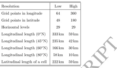
Resolution Low High
Grid points in longitude 64 360
Grid points in latitude 48 180
Horizontal levels 29 29
Longitudinal length (0◦N) 333 km 59 km
Longitudinal length (45◦N) 235 km 42 km
Longitudinal length (60◦N) 166 km 30 km
Longitudinal length (80◦N) 58 km 10 km
Latitudinal length of a cell 222 km 59 km
Table 1: Table of the main geometric features for the two resolutions of the study: number and size of cells.
insights can be gained into the water cycle and global climate from high-resolution simulations?
35
In section 2, we present the global climate model used in this study, and describe the simulations that were carried out. In section 3, the impact of the increase in resolution on the dynamics of the atmosphere and on the simulated thermal structure is studied. Then we focus in section 4 on the water cycle, using seasonal simulations performed over a whole year. In particular, planetary wave structures and their effect on clouds and vapor are investigated in section 5. Finally we study the sublimation processes on the northern
40
polar cap, the main water reservoir, in section 6. Working at high resolution means resolving the cap better, with, for example, a better rendering of Chasma Boreale on topographical profiles. This has an effect on the water cycle and on the climate.
2. Methodology
2.1. The LMD global climate model
45
The model used in this study is the martian global climate model of the Laboratoire de M´et´eorologie Dynamique (Forget et al., 1999). It is able to model a comprehensive water cycle for the red planet. The ability to simulate radiatively active clouds is included in the model (Madeleine et al., 2012a) (radiatively active clouds will also be called RAC in this paper). The cloud model includes a microphysical scheme that models the growth of water ice crystals onto dust nucleation cores (Montmessin et al., 2002), and whose
50
effects on the climate are described in Navarro et al. (2014). Fluid mechanics equations for the atmosphere are solved in a finite-difference grid point dynamical core. A spatial polar filter is used in the GCM to remove small scale waves which irrealistically accumulate energy due to the limitation in scale caused by the finite grid cells. The polar filter removes some numerical instabilities. Dust, ice, vapor and condensation nuclei are tracers that can be advected in air parcels. The dust vertical distribution and the dust particle
55
ACCEPTED MANUSCRIPT
column opacity is prescribed using observation-derived dust “scenarios” detailed in Montabone et al. (2015). This means that the climate of a particular martian year can be computed. Unless otherwise indicated, the runs presented in this paper were performed with the scenario for Martian year 26 from Montabone et al. (2015). The study of interannual variability of traveling waves and water transport is beyond the scope of
60
this paper.
2.2. Simulated cases
The standard resolution grid in previous studies of the water cycle with the LMD GCM makes use of 64 longitude per 48 latitude cells, with 29 vertical layers (Montmessin et al., 2004; Madeleine et al., 2012a; Navarro et al., 2014). Using the same number of vertical layers, with a model top at an altitude of about
65
80 km, this study aims at comparing these standard low resolution simulations (5.625◦× 3.75◦) with model
runs performed with a higher horizontal resolution (1◦× 1◦). Closer to the poles, one degree in longitude
represents a smaller arc of a circle (Table 1), whereas one degree in latitude represents the same distance on the ground (59 km). This means that the surface area of a grid cell decreases closer to the poles. A
polar filter limits effective longitudinal resolution of waves to the resolution at 60◦N. The improvement in
70
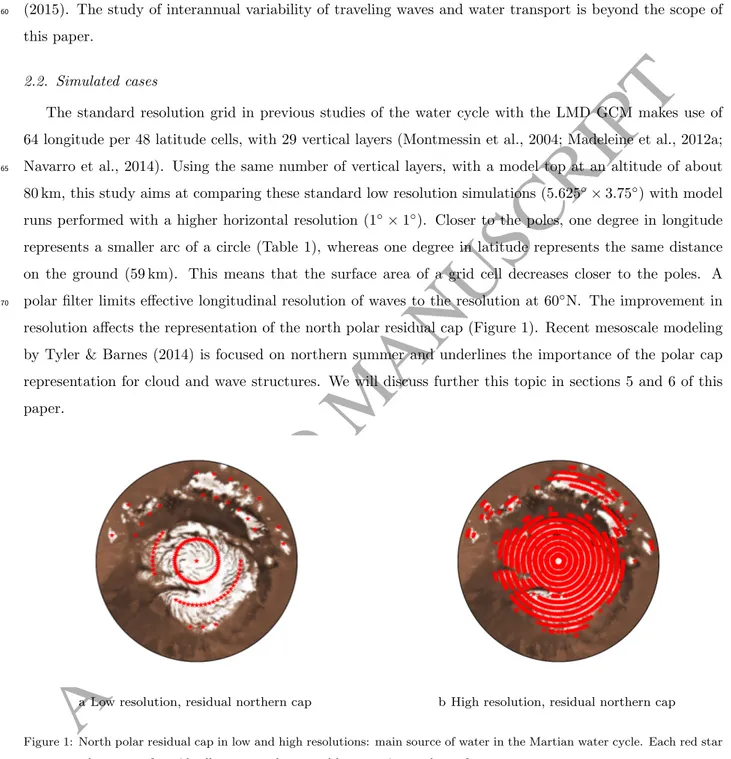
resolution affects the representation of the north polar residual cap (Figure 1). Recent mesoscale modeling by Tyler & Barnes (2014) is focused on northern summer and underlines the importance of the polar cap representation for cloud and wave structures. We will discuss further this topic in sections 5 and 6 of this paper.
a Low resolution, residual northern cap b High resolution, residual northern cap
Figure 1: North polar residual cap in low and high resolutions: main source of water in the Martian water cycle. Each red star represents the center of a grid cell permanently covered by water ice on the surface.
To compute an initial state for the high-resolution simulations, a lower resolution state from a simulation
75
ACCEPTED MANUSCRIPT
the north pole was inferred from a thermal inertia map of Mars. Where thermal inertia, taken from data (Mellon et al., 2000; Wilson et al., 2007), is higher than 500 J m−2K−1s−1
2, model cells are set to be part
of the water ice deposits. Topography (Smith et al., 2001a) and albedo (Christensen et al., 2001) maps at higher resolution are also used. Figure 1 shows the resulting map of the pole. The northern perennial ice cap
80
has a surface of AHR= 1.27× 10⁶km2 at high resolution, while it has a surface of ALR= 9.91× 10⁵km2 at
low resolution. As AHR= 1.28×ALR, the area of exposed water ice is consequently larger at high resolution.
Low resolution runs are converged, while high resolution ones were only run for one year. For high resolution runs, work was done when preparing the runs to make the transition from low to high resolution topography smooth, removing irrealistic amounts of ice deposited where no perennial cap is observed. These areas are
85
key to convergence. At the end of the year, the water vapor amount does not diverge that much compared to the beginning.
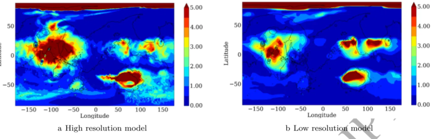
To understand the scales involved, Figure 2 shows two maps of the total cloud ice column at the time of
the northern summer solstice (Ls= 90◦), in the low and high resolution simulations with radiatively active
clouds. The observed fine-scale structure (“patchiness”) of clouds is better resolved in the high-resolution
90
run. There is a global increase of cloud thickness. Furthermore, the thick clouds in Hellas (> 5 pr. µm) fill only the northern part of the basin at low resolution, whereas they encircle the edge of Hellas and spread to
the west in the high-resolution simulations. In the area between 60◦E and 180◦E, east and south of Hellas,
there is a wide area of textured clouds that extends as far as the south pole, that are not present in lower
resolution runs. More clouds appear over Argyre and overall south of 50◦S. Such maps can be compared
95
to Mars Orbiter Camera pictures depicting water ice clouds in shades of blue (Wang & Ingersoll, 2002). Clouds on Mars on orbiter pictures during daytime are really textured and are anchored to topographical features like Tharsis Montes. Fog is present inside Valles Marineris and Hellas on MOC orbiter images at a local time of 2 P.M. The fragmentation of clouds in high-resolution runs tends to match MOC images more closely. However the aphelion season in high latitudes in the north and south tends to be too cloudy in
100
the LMD MGCM (clouds are too thick, both during the day and the night), compared to MCS (McCleese et al., 2010) and TES data (Smith et al., 2001b). Faint nighttime low-latitude clouds seem more widespread in observations (MCS data, again) than in the LMD GCM model. Data showing the winter polar hood is difficult to obtain, but for example nighttime TES data (Pankine et al., 2013) in northern winter shows that the edge of the polar hood qualitatively agrees with the LMDZ Mars model (simulated clouds having the
105
tendency to spread a bit further south, though). Pankine et al. (2013) could not observe well the core of the polar hood due to a lack of thermal contrast. Figure 2 of Navarro et al. (2014) shows that the simulated polar hood clouds are thicker than indicated in TES diurnal observations. We will discuss in section 4 how resolution affects this result.
To better pinpoint resolution effects, low (LR) and high resolution (HR) versions of the model were also
110
ACCEPTED MANUSCRIPT
a High resolution model b Low resolution model
Figure 2: A comparison of two maps of the column of atmospheric water ice (in pr. µm) at the northern summer solstice as modeled by the LMD Mars GCM at high and low resolution (see Table 1). Midnight is at longitude 0. Contours of MOLA topography (black lines) show main surface features at 1◦× 1◦for both maps.
ambiant infrared and visible radiation in the atmosphere of the planet. The non-linear thermodynamical effects caused by the interaction between airborne ice particles and light are suppressed (Navarro et al., 2014). The modification of water sources at the different resolutions changes the water cycle, but these changes are amplified by the radiative effect of clouds, owing to positive and negative feedbacks between
115
atmospheric dynamics, cloud formation, and the impact thereof on the thermal structure. The inactive runs conducted in this study, at both high and low resolutions, help untangle the phenomena. Inactive runs are less realistic (Madeleine et al., 2012a; Navarro et al., 2014), as will be confirmed later in the paper.
3. Vertical structure: atmospheric profiles and thermal tides
The aim of this section is to review the impact of resolution on the average vertical structure of the
120
atmosphere, studying temperature profiles, and the link with cloud content, vapor profiles, and dust loading. Profiles, averaged over all longitudes (zonal mean) and over twenty days, are studied. They help quantify exactly the effect of resolution, with or without radiatively active clouds.
3.1. Runs without radiatively active clouds
Overall, high- and low-resolution cases without radiatively active clouds (or HRIC and LRIC cases) are
125
quite similar, except for the polar warming in the polar night, which is known to be model dependent (see Figures 8 and 9 of Forget et al. (1999)) and notably sensitive to resolution (Toigo et al., 2012).
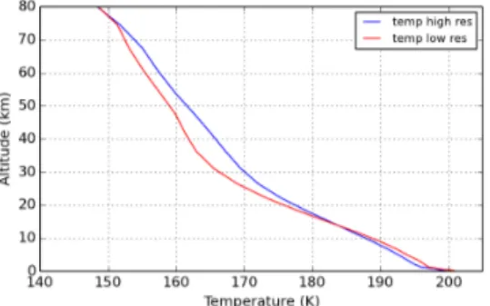
Figure 3 shows temperature and water vapor profiles from LRIC and HRIC runs. The yearly average profiles of temperature for the whole planet are very similar, with a slightly colder higher atmosphere
(40− 100 km) in the high resolution case. The temperature inversion is a consequence of the adiabatic
130
ACCEPTED MANUSCRIPT
with a 7 K increase in high altitudes at high resolution. At the South pole at its winter solstice, the high
resolution model is colder at high altitudes. This is confirmed at Ls = 270◦: the air is warmer at high
altitudes above the winter pole in low resolution, which means the Hadley cell circulation slightly decreases in activity with the increase in resolution in the IC case. The annual averages of the dust profiles in the
135
atmosphere (figure not shown) show little difference from run to run because of the prescribed dust loading read in the dust scenarios from data. Relative shifts could however happen between high and low altitudes. IC runs do not show any significant relative increase in dust loading in middle-to-high altitudes (10 to 40 km) and cannot explain the differences in temperature.
Yearly averaged cloud formation seems confined within the 10− 40 km height range with a peak around
140
15 km and 35 km, within the altitude range of clouds in published simulations and observations (Madeleine et al., 2012b; Wilson & Guzewich, 2014). Within the tropics there is an increase in vapor content in the lowest layers, and a smaller increase in cloud content. The southern polar hood at the winter solstice is thicker than at low resolution.
Terrestrial planets with a diurnal cycle and an atmosphere like the Earth or Mars are subject to diurnal
145
and semi-diurnal (harmonics of the diurnal cycle) waves. The sun heats periodically different areas of the planet and the atmospheric system responds to this forcing by producing waves. Lindzen (1970) presents an early discussion of the application of the Earth tidal theory to Mars. Tidal waves have been studied on Mars, for example, recently, using Mars Climate Sounder data (Kleinb¨ohl et al., 2013). These thermal tides are a key element of the global atmospheric dynamics on Mars. Overall, the latitudinal structure of the
150
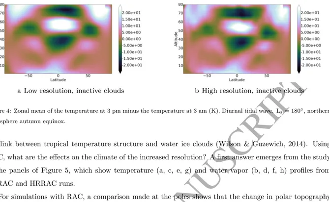
thermal tides is found to be almost insensitive to horizontal model resolution with an alternance of extrema where afternoon temperature is higher than night temperature and the reverse. On Figure 4, the zonal mean temperature at 3 P.M. minus the temperature at 3 A.M. (the local times observed by Mars Climate Sounder) is shown in an altitude versus latitude plot for high and low resolutions (without active clouds).
The time period is a snapshot of Ls= 180◦. This structure evolves slowly during the year. These graphs
155
are comparable to similar plots derived from MCS data (Figure 4 of Guzewich et al. (2012), or Figure 3 of Lee et al. (2009)).
3.2. Runs with radiatively active clouds
The IC runs show a rather unrealistic cloud cover. At first clouds were thought not to affect the martian climate, being only a byproduct of its effect on the water cycle. However, cloud coverage affects the climate,
160
as water ice clouds interact mostly with thermal radiation, absorbing and scattering it. There is a quantifiable effect on air and surface temperature via the greenhouse effect when the clouds are thick or high enough or both (Madeleine et al., 2012a). For example, RAC in summer in the northern hemisphere are responsible for higher nighttime surface temperatures under the aphelion cloud belt due to the supplementary infrared radiation (Wilson et al., 2007). Temperature inversions above Tharsis where clouds are the thickest show
ACCEPTED MANUSCRIPT
a T, yearly average, all latitudes b H2O, yearly average, all latitudes
c T, 30°N to 30°S, 20-sols mean around Ls= 90° d H2O, 30°N–30°S, 20-sols mean at Ls= 90°
e T, 75° to 90°N, 20-sols mean around Ls= 90° f H2O, 75°–90°N, 20-sols mean at Ls= 90°
g T, 75° to 90°S, 20-sols mean around Ls= 90° h H2O, 75°–90°S, 20-sols mean at Ls= 90°
Figure 3: Vertical profiles of temperature T (K), water mixing ratio of ice and vapor (mol/mol), zonally averaged, simulations with inactive clouds. Blue curves: high-resolution run, red curves: low-resolution run.
ACCEPTED MANUSCRIPT
a Low resolution, inactive clouds b High resolution, inactive clouds
Figure 4: Zonal mean of the temperature at 3 pm minus the temperature at 3 am (K). Diurnal tidal wave. Ls= 180◦, northern
hemisphere autumn equinox.
the link between tropical temperature structure and water ice clouds (Wilson & Guzewich, 2014). Using RAC, what are the effects on the climate of the increased resolution? A first answer emerges from the study of the panels of Figure 5, which show temperature (a, c, e, g) and water vapor (b, d, f, h) profiles from LRRAC and HRRAC runs.
For simulations with RAC, a comparison made at the poles shows that the change in polar topography
170
and ice distribution is reflected in the atmosphere as the water sublimates. There is more water released in the atmosphere (Figure 5f) at high resolution, the origin of which is surface ice sublimation. The increased ice sublimation results from a longer period of absence of polar hood, and better evacuation of water from the polar areas by air circulation within atmospheric cells and winds over the cap (see later subsections for details). While the LR profile exhibits a drop in water vapor near the ground, reflected in an increase in
175
cloud mass below 10 km, clouds are less thick at high resolution and their peak is higher in altitude. This reflects the earlier and more gradual disappearance of the polar hood (described in subsection 4). This affects temperature (Figure 5e): the polar hood cools the lower levels more intensively at low resolution, and both the low altitude and high altitude temperature inversions are not present at high resolution, while the temperature gradient is also less steep.
180
The increase of water vapor inventory has an effect on the aphelion tropical climate (Figure 5c), because thicker and more spatially extended clouds form by adiabatic cooling out of the wetter air masses traveling from the pole to the northern tropics (Figure 5d). The temperature profile is warmed up to an altitude of 50 km and is then colder above in the high-resolution run. This results from a strengthening of the Hadley cell circulation, induced by the radiative effect of clouds (Wilson et al., 2008; Madeleine et al., 2012a), that
185
in turn increases the cloud cover.
Averaged over the whole year and the whole planet (Figure 5b), the main result is an overall wetter atmosphere, in HR simulations, as more water is advected from the north polar cap. The air is noticeably drier in the upper atmosphere without the radiatively active clouds. This produces thicker clouds that also
ACCEPTED MANUSCRIPT
a T, yearly average, all latitudes b H2O, yearly average, all latitudes
c T, 30°N to 30°S, 20-sols mean around Ls= 90° d H2O, 30°N–30°S, 20-sols mean at Ls= 90°
e T, 75° to 90°N, 20-sols mean around Ls= 90° f H2O, 75°–90°N, 20-sols mean at Ls= 90°
g T, 75° to 90°S, 20-sols mean around Ls= 90° h H2O, 75°–90°S, 20-sols mean at Ls= 90°
Figure 5: Vertical profiles of temperature T (K), water mixing ratio of ice and vapor (mol/mol), zonally averaged, simulations with radiatively active clouds. Blue curves: high-resolution run, red curves: low-resolution run.
ACCEPTED MANUSCRIPT
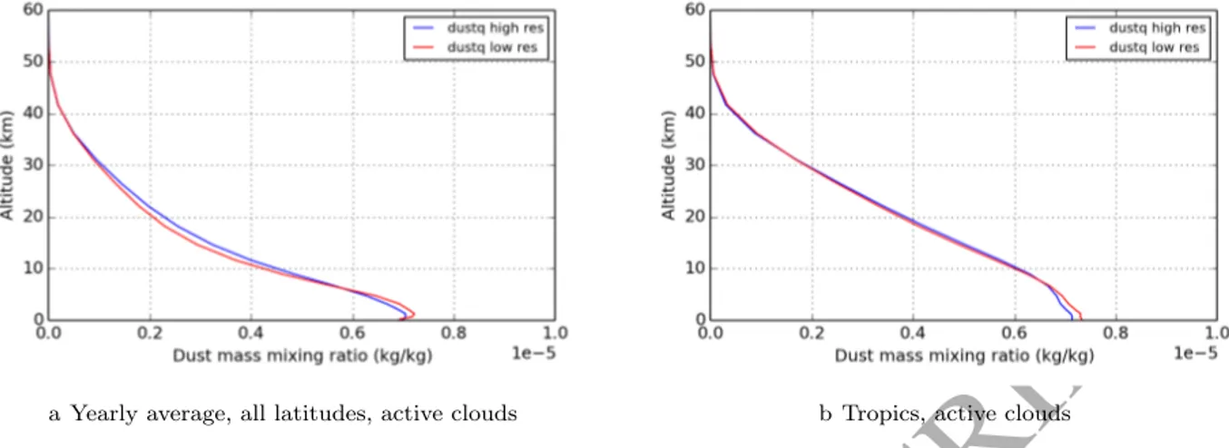
a Yearly average, all latitudes, active clouds b Tropics, active clouds
Figure 6: Profiles of dust mixing ratio (kg/kg), averaged over a year and zonally, as a function of altitude above areoid. Blue curves: high-resolution run, red curves: low-resolution run.
cover more area, especially during the aphelion season with its cloud belt (Figure 5d, see section 4). These
190
clouds have an impact on the Hadley cell circulation, which is strengthened. This results in dust transported to higher altitudes, with a dust depletion at lower altitudes, as can be seen on the yearly averaged dust profile shown on Figure 6a and b. The dust-cloud feedback is described in Kahre et al. (2015). However, the globally averaged vertical distribution of dust is only very slightly changed.
The winter south pole has more water vapor (at high resolution) incoming through high latitudes from
195
the Northern hemisphere, that condenses as clouds below 40 km. There was no water transport of this magnitude in both previously studied LRIC and HRIC runs. Ice is consequently deposited by sedimentation onto the seasonal cap (see Figure 5h). The low altitude temperature gradient remains the same (following
CO2condensation temperature) while at high altitude there is an increase of 30 K of the peak temperature.
A temperature of 170 K over the South Pole has been observed in the data, later in the soutern winter: see
200
Figure 25 of Kleinb¨ohl et al. (2009).
The strengthening of the temperature inversion over the South pole in winter is a symptom of the strengthening of the Hadley cell in the HR run. Indeed, this air is adiabatically heated in the descending branch of the cell which rises in the summer hemisphere (Forget et al., 1999). It contrasts with the behavior of the inactive runs that get colder in high altitudes in the high resolution runs.
205
In general, thermal inversion is less marked than in the inactive runs. Cloud and vapor content are enhanced in the active runs as compared to the inactive ones: RAC amplify this change, like catalysts. There is an averaged hotter higher atmosphere in the HR case, which is the opposite of what is observed with IC. Resolution does not change deeply the thermal structure, except in polar areas, (as expected, see 8 of Forget et al. (1999)), as Hadley circulation affects heating in polar areas and thermal effects are
210
ACCEPTED MANUSCRIPT
RAC. During the northern fall equinox, the high altitude north-to-south wave amplitude is greater at high
resolution, especially the 30◦S-30◦N latitude zone at a height of 80 km (Figure 7). This corresponds to the
dominant mode, which has a phase reversal at 22◦S and 22◦N (Zurek, 1976; Lee et al., 2009). The difference
between the thermal tide of the active and inactive cloud models is reduced at high resolution. Previous
215
works have shown that RAC increase the amplitude of the semidiurnal tide (Wilson et al., 2014). Wilson & Guzewich (2014) have shown that, as compared to IC simulations, RAC tend to heat the air in the night above 100 Pa, and cool it at 200 Pa near the base of the cloud deck, during the aphelion season. Here, a noticeable fact is that the vertical wavelength of the thermal tide is increased by about 10 km in active cloud simulations, showing the thermal effects of the clouds. At high latitudes, between 60 and 80 km, the wave
220
structure shows high-frequency perturbations. The tidal waves in HR simulations are overall consistent with LR simulations with RAC. The waves excited by the alternating sunlight and nighttimes are typically the same, to first order. High in the sky (> 70 km), the zonal wave amplitude is bigger in the high resolution simulation, and below, it tends to be a bit smaller. High resolution also allows fragmentation into smaller scale perturbations at high latitudes/altitudes. With RAC, horizontal resolution does not seem to impact
225
the vertical wavelength of the tide, which is an improvement if we compare to the inactive cases (where the vertical wavelength shrinks when resolution improves).
a Low resolution, active clouds b High resolution, active clouds
Figure 7: Zonal mean of the temperature at 3 pm minus the temperature at 3 am (K). Diurnal tidal wave. Ls= 180◦, northern
hemisphere autumn equinox.
4. Discussion: impact on the water cycle
In section 3, we discussed the thermal variation in active runs, the strengthening of the Hadley cell circulation, and the consequences on cloud thickness and height. The precise effect on the water cycle,
230
considering the atmosphere of Mars as a system with its reservoirs and transport vectors is discussed here and in the following sections. The column integrated amount of water vapor in the atmosphere, as presented in Figures 8 and 9, is a proxy for water cycle activity on the planet. At high resolution, with active clouds,
ACCEPTED MANUSCRIPT
from north to south in southern summer is less steep at high resolution than at low resolution. This has
235
an impact on the “Clancy” effect, as described in Clancy et al. (1996), explaining the asymmetry between northward and southward global transport of water by the trapping of water by the aphelion cloud belt. That non-linear coupling between circulation and cloud formation describes how the quantity and advection of water in the aphelion summer hemisphere is enhanced as the eccentric orbit affects water vapor saturation altitude.
240
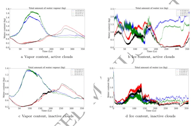
a Vapor content, active clouds b Ice content, active clouds
c Vapor content, inactive clouds d Ice content, inactive clouds
Figure 8: Total water ice and vapor content (kg) of the two martian hemispheres for one year, for runs with (top) and without (bottom) active clouds. In blue and red are the high-resolution masses of water in the northern and southern hemisphere respectively, while in green and black are the lower resolution northern and southern masses of water.
The total water budget for the two hemispheres allow us to assess the sensitivity to resolution of in-terhemispheric water distribution for inactive cloud simulations (figures not shown). A comparison can be made, for example, with the same inventory made with Viking data, see Figure 6 of Jakosky & Farmer (1982). This allows us to understand how the water distribution evolves throughout the year and the differ-ences between the models that were run, at high and low resolutions. The total hemispheric water content
245
illustrates the differences between the two models (see Figure 8). The mass of water vapor has an order of
magnitude of 1012 kg, while the order of magnitude of the ice mass is 1011 kg. As a rule of thumb, ice in
the atmosphere represents 10 % of the water available.
On Figure 8a the total amount of water vapor by hemisphere is shown for the RAC simulations. There are two main peaks which originate from the sublimation of the seasonal frost in summer. The first one, in
ACCEPTED MANUSCRIPT
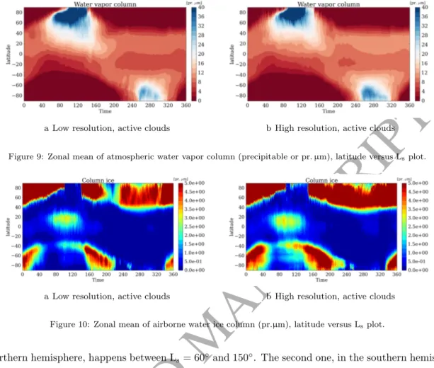
a Low resolution, active clouds b High resolution, active clouds
Figure 9: Zonal mean of atmospheric water vapor column (precipitable or pr. µm), latitude versus Ls plot.
a Low resolution, active clouds b High resolution, active clouds
Figure 10: Zonal mean of airborne water ice column (pr.µm), latitude versus Lsplot.
the northern hemisphere, happens between Ls= 60◦and 150◦. The second one, in the southern hemisphere,
peaks between Ls= 240◦ and 320◦. The crossing of curves at Ls= 200◦ corresponds to the shifting of the
water dominance from the north to the south as northern polar dusk falls. The high resolution maximum
water content is 0.2× 10¹²kg lower in the north than the lower resolution one. However there is more
water vapor available in the southern hemisphere. These graphs can be compared to TES hemispheric water
255
vapor data, figure 8 of Smith (2002), which shows a northern hemisphere maximum of more than 2× 10¹²kg
and a southern hemisphere maximum of 1.5× 10¹²kg. These early results were later adjusted with a 40%
decrease in the northern peak, more in agreement with PFS results (Fouchet et al., 2007). This means
the aforementioned maxima become 1.2× 10¹²kg (north) and 0.9
× 1012kg (south) respectively. These
values show that the HRRAC simulation is closer to the observations in the northern hemisphere wet season
260
(1.4× 10¹²kg of vapor at the peak instead of 1.7
× 1012kg value of LRRAC simulations). In the southern
hemisphere, the HRRAC simulations are too wet with a peak at 1× 10¹²kg instead of 0.8× 10¹²kg of the
LRRAC simulations. Another set of observations, SPICAM (Trokhimovskiy et al., 2015), giving total mass
of water on the whole planet, shows a too dry HRRAC model in the aphelion season (2.1× 10¹²kg are
observed) and a too wet HRRAC model in the southern spring and summer (1.3× 10¹²kg). As for water
265
ACCEPTED MANUSCRIPT
Indeed, there is an increase of 0.5× 10¹¹ kg of cloud amount in the south in the HR run as compared to
the LR one. And this difference is also found in the northern hemisphere in winter with roughly the same amplitude. The total amount of water ice also begins its northern fall increase earlier with a smaller increase. Active cloud simulations are drier at low latitudes, either at high or low resolution, as compared to IC
270
runs (Figures 8c and d). Polar ice sublimation is more efficient (as compared to IC runs) in northern and
southern summer north of 60◦N and south of 60◦S. There are more clouds everywhere and during the whole
year, these clouds are thicker. This is due to the reduced content of water released in the atmosphere in IC runs. Also, with RAC, when clouds appear at low altitudes, these clouds reflect the incoming sunlight and tend to further cool the atmosphere, resulting in even more clouds. But clouds at high altitudes absorb
275
thermal radiation from the planet and emit at that colder temperature: they should rather have a warming effect. This feedback loop is described in Navarro et al. (2014), for example. Kahre et al. (2015) explores the relationship between this feedback loop and the dust cycle, impacting polar warming.
With active clouds, resolution primarily influences the northern polar hood (see figure 10). At high resolution, the disappearance of the polar hood happens earlier and the cloud-free period around summer
280
solstice lasts longer, possibly because the higher resolution affects daytime duration, with a finer terminator representation. However there are transient polar clouds that are able to form locally. The polar hood is overall thicker. The study of baroclinic waves, in section 5, sheds light on atmospheric dynamics phenomena that can explain these differences. Yet again, it is apparent that the clouds’ interaction with incoming and outgoing radiation is key to the organization of the fluxes of water.
285
Assessing the realism of the polar hood simulations can be difficult. The observed thickness of the polar hood is difficult to assess (see also section 2.2). The thick polar hood clouds of RAC simulations seem unrealistic if we compare them to what we can see of the polar hood (i.e, its edge) in MCS or nighttime TES data (Pankine et al., 2013). But there is an observational bias that must be taken into account: the lack of thermal contrast affects the visibility of clouds from the heart of the polar hood. Temperature data can also
290
be used to try to understand indirectly which simulation is more realistic. Unlike for the tropical clouds, it is not easy to use surface temperature to constrain the characteristics of the polar hood clouds, for three
reasons. The ground under the polar hood clouds is covered by CO2 ice. Surface temperature data may be
affected by the presence of the clouds. In the regions where the polar hood forms, the difference between the modeled and observed temperatures seems to mostly result from the error in the timing of the modeled
295
CO2ice cap. The effect of the clouds is small compared to this error. Thus it prevents us from assessing the
realism of our cloud simulation. So, we have tried to look at low altitude temperatures to compare them with data. Global low altitude temperatures seems lower in RAC simulations. Thicker clouds seem to have a global cooling effect. However, a more detailed study shows that this depends on the time of the day, and on the altitude and thickness of the clouds. McCleese et al. (2010) (Figure 4) shows polar temperatures
300
ACCEPTED MANUSCRIPT
temperature inversion seem close to our results with RAC in the north polar winter (low or high resolution, figure not included in the paper). The temperature maxima seem to have a slightly higher altitude in the data, and the HRIC run, with its colder (170–180 K) temperature maximum, matches better the data than the LRIC. With RAC, the HRRAC and LRRAC are closer to each other, and both agree rather well with
305
the data during the north polar winter, qualitatively. As for the south polar hood, comparing Figure 5g and the MCS data, the HRRAC model matches the data better with its peak of temperature inversion at 170 K rather than the 140 K of the LRRAC (which is too cold). Madeleine et al. (2012a) has shown that in the LMD GCM the low level clouds cool the atmosphere at the poles (especially at equinoxes). The loss of infrared radiation to space makes the lower atmosphere near the north pole too cold by 15 K in early spring,
310
for example. This corrects a previous warm bias (so IC simulations are not realistic either with their too thin clouds) (Madeleine et al., 2012a), but replaces it by a cold one.
HR runs tend to be more cloudy, especially in the winter hemisphere. One hypothesis would be that polar hood edge dynamics, with a better resolved latitudinal temperature gradient, allow the formation of smaller ice particles due to smaller supersaturation and slower growth of crystals. These smaller ice particles
315
stay longer in the atmosphere. Stronger baroclinic waves (see later) also inject more easily water toward the pole and thus increase cloud quantity and coverage.
This shows the key part the active clouds take in atmospheric dynamics and their impact on the water budget. Overall there is more water everywhere and at all times, and the behavior of clouds is more erratic and different from one run to another, which is compatible with the presence of a feedback loop between
320
temperature, water vapor and clouds. Indeed, RAC GCM runs are more sensitive to model parameters, because of a positive feedback between cloud formation and temperatures (Navarro et al., 2014), and more unstable.
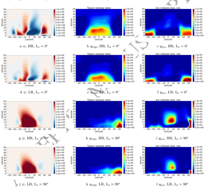
To further analyze the water cycle behaviour described in the paragraphs above, we show Figures 11 and 12 mean zonal stream functions, and water vapor and ice mixing ratios, all for the HRRAC and LRRAC runs
325
and for all seasons. At Ls= 0◦, at high resolution, there is an intensification of the low- to middle-latitude
circulation in the northern hemisphere, and also in the high-latitude cell in that same hemisphere. This results in an increase in the amount of water vapor, especially at higher altitudes. The aphelion cloud belt
is thicker, while there are less clouds near the north pole. At Ls = 90◦, the global north-to-south cell is
strenghtened with the increase in resolution, which results in more vapor above the north pole, and most
330
of all a wider vertical extension of the polar hood clouds. The aphelion cloud belt is thicker, which tends
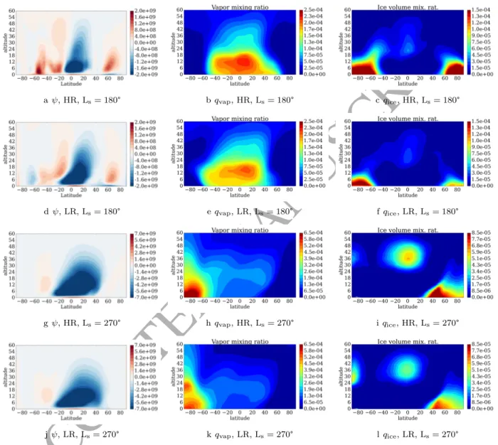
to reduce the amount of water vapor present at lower latitudes. At Ls = 180◦ , polar hoods are thicker
and have a greater vertical extension at high resolution. The middle- to low-latitude clouds are also thicker. Polar cells are strengthened. On the whole, there is more water vapor, but it is more spatially confined due
to the high-latitude cells. Middle to low latitudes are wetter at high resolution.At Ls = 270◦, again, the
335
ACCEPTED MANUSCRIPT
at the south pole, the atmosphere is wetter, not only at the pole but also above the middle to low latitudes. All clouds are thicker, except those high above the south pole. The double maxima of water vapor above the south pole merge at high resolution.
To conclude this study of mean meridional circulation, the fact that there is a global strengthening
340
of the Hadley cell circulation is confirmed, especially at solstices. The transition cells of the equinox are more complex, but show globally the same trend of a wetter and clouder atmosphere. Evolutions in cell morphology have consequences on the confinement of vapor and clouds and on the localization of maxima.
a ψ, HR, Ls= 0° b qvap, HR, Ls= 0° c qice, HR, Ls= 0°
d ψ, LR, Ls= 0° e qvap, LR, Ls= 0° f qice, LR, Ls= 0°
g ψ, HR, Ls= 90° h qvap, HR, Ls= 90° i qice, HR, Ls= 90°
j ψ, LR, Ls= 90° k qvap, LR, Ls= 90° l qice, LR, Ls= 90°
Figure 11: Mean zonal stream function (kg/s), water vapor (qvap) and ice (qice) mixing ratio (mol/mol), for the high- (HR)
ACCEPTED MANUSCRIPT
a ψ, HR, Ls= 180° b qvap, HR, Ls= 180° c qice, HR, Ls= 180°
d ψ, LR, Ls= 180° e qvap, LR, Ls= 180° f qice, LR, Ls= 180°
g ψ, HR, Ls= 270° h qvap, HR, Ls= 270° i qice, HR, Ls= 270°
j ψ, LR, Ls= 270° k qvap, LR, Ls= 270° l qice, LR, Ls= 270°
Figure 12: Mean zonal stream function (kg/s), water vapor (qvap) and ice (qice) mixing ratio (mol/mol), for the high- (HR)
ACCEPTED MANUSCRIPT
5. Baroclinic waves and the polar hood 5.1. Spectral analysis of baroclinic waves
345
Baroclinic waves shape the water transport on Mars at midlatitudes. In Barnes (1980, 1981), pressure data from the Viking 1 (22.5◦N, 48◦W) lander, and all data types from the lander 2 (48◦N, 226◦W), were used
to infer dynamical properties of eastward traveling transient disturbances caused by baroclinic instability
(Ls= 180–360◦). The two dominant spectral peaks of disturbances were calculated to have wavenumbers
of 2 to 4. Periodicity was about 3.1 sol and 6 to 8 sol. Reduced activity was noted around Ls= 280–313◦
350
during wintertime. Barnes (1981) confirmed the first results, and also detected baroclinic waves centered to the north of the Lander 2 site. The 6–8 sol periodicity has a zonal wavenumber of 1.5–2, and the higher frequency peak (2 to 3 sol) tends to have a higher wavenumber (3–4). The onset of dust storms seems to strengthen atmospheric heating during the day, and strengthen the diurnal cycle signature, decreasing the signal of baroclinic waves.
355
The instrument TES aboard the MGS spacecraft provided a more complete dataset for the study of waves. TES nadir temperature data revealed zonal wavenumbers 1 and 2 waves, the former, prominent at the winter solstice, being bimodal, with a slow higher altitude wave (periods of more than 10 sol) and a fast surface wave (period of 6–7 sol), the latter, dominant in autumn or spring, having periods of 3–4 and 6–7 sol (Banfield et al., 2004). MGS MOC data and MGS radio occultation data confirmed the presence of
360
a dominant eastward-travelling wave with zonal wavenumber 3, and secondary ones at 2 and 1, all three having a period of 2.3 sol (Hinson & Wang, 2010), plus a wavenumber 2 stationary wave (Rossby wave that
shapes the polar hood clouds). Shifts in frequencies were observed around Ls= 230◦ from a period of 2 to
3 sol for zonal wavenumbers 1 to 3 waves (Hinson & Wang, 2010). In Hinson et al. (2012), MGS TES and Radio Science experiment data were used to analyze the triggering of regional dust storms in the northern
365
hemisphere basins by the zonal wavenumber 3 mode. Indeed, zonal wavenumbers of 1 to 3 exist, with the mode 3 having the smallest periods (2–3 sol), and the mode 1 the longest (P > 6 sol). Baroclinic wave modes are anticorrelated; when one is strong, others tend to be weak, and longer waves of zonal wavenumber 1 or 2 tend to have deeper vertical structure than the shorter ones. A mode tends to stay coherent for 15 to 30 sol (Hinson et al., 2012). Traveling dust storms may symmetrically and non-linearly enhance the zonal
370
wavenumber 3 traveling waves under specific conditions according to global climate simulations (Wang et al., 2013).
Lewis et al. (2016) used MGS TES assimilation inside the LMD/UK GCM and explored the repeatable pattern of wave decrease around solstices, when low altitude transient waves reach a minimum around winter solstice, while thermal contrast between the summer hemisphere and the winter pole is maximal.
375
This solsticial pause is most visible in wavenumber 2 to 3 waves (stronger in spring and autumn) while wavenumber one waves are rather prominent near the solstice (Lewis et al., 2016). GCM sensitivity studies
ACCEPTED MANUSCRIPT
are important as the interaction with topography seems to greatly influence the rise of different wavenumbers in spectral studies of the baroclinic waves. Indeed, by modification of near surface flow, the zonal variations of topography weaken transient eddies around solstice in both hemispheres (Mulholland et al., 2016). The
380
intercomparisons between inactive and RAC simulations are revealing as RAC are known to increase low-level winds of the eastward propagating waves of periods of 1.5 to 10 sol, as their radiative cooling within the polar hood in spring and fall seasons influences the structure of the polar vortex (Wilson, 2011). They are also known to play a role in the dampening of baroclinic waves around winter solstices, due to a decrease of the vertical shear of the westerly jet near the surface around solstices, see also section 5.3 (Mulholland et al.,
385
2016). In this section, we will study Fourier transforms of the waves that are visible in the LRIC, HRIC, LRRAC and HRRAC models to analyze how harmonics of the transient eddies are respectively impacted by horizontal resolution and RAC: Figures 13 and 14 show the Fourier transform of the surface pressure at two latitude ranges for northern fall and winter (Ls= 180◦ to 360◦) waves.
Impact of radiatively active clouds. At 48◦N (the Viking lander 2 location, Figure 13), RAC result in the
390
shifting of the dominant frequency and wavenumber from 0.17 sol−1(wavenumber 1 to 2) to 0.4 sol−1(2.5 sol
period). The frequencies are consistent with the slow and fast waves observed in Viking data, with a trend of
higher frequency for higher wavenumbers (Barnes, 1981). At higher latitudes (70◦N to 80◦N latitude band,
Figure 14) the shifting is opposite as modes from 0.05 to 0.15 sol−1 become populated at high resolution,
while inhibited in HRIC simulations. At the Viking lander 2 latitude, and thus further to the south, waves
395
tend to exhibit higher wavenumbers (see for exemple the 0.17 sol−1waves). The waves propagate more slowly
than in the inactive run. Wavenumber 2 waves seem to widen and lean towards wavenumber 1 at higher frequencies. For RAC simulations, westward waves appear (they are only very faintly present in the HRIC
run). The wavenumber is−1 (westward), and the peak frequency is at 0.1 sol−1(10 sol). Comparing IC and
RAC runs, there are more harmonics in the active run, and more wave frequency dispersion. Irregularities
400
in the baroclinic instabilities are the consequence of the cloud feedback that intercepts outgoing radiation. Non linear effects and positive feedback loops in active clouds seem to favor the wavenumber 1 waves. Effect of resolution. The recurring most prominent feature of the spectra is the peak at a frequency of
0.17 sol−1 (5.9 sol period), with a wavenumber 1 in most of the cases. There is also an ubiquitous weaker
family of waves of wavenumber 2 at a frequency of about 0.38 to 0.55 (2.6 to 1.8 sol−1). High resolution
405
populates the spectra with higher frequency and wavenumber oscillations, as a wider range of waves is generated by the increased irregularities and chaos, see for example Figure 13; in IC runs the high frequency peak becomes bimodal at high resolution with frequencies of 0.38 and 0.45 (2.6 and 2.2 sol respectively). The westward waves are enhanced by higher resolution. More frequency dispersion also appears in HR runs compared to the LR ones. The more detailed topography and smaller scale phenomena interaction cause
ACCEPTED MANUSCRIPT
Figure 13: Two dimensional Fourier transform of the surface pressure variable (Pa) for the period Ls = 180◦–360◦, colorbar
ACCEPTED MANUSCRIPT
Figure 14: Two dimensional Fourier transform of the surface pressure variable (Pa) for the period Ls = 180◦–360◦, colorbar
ACCEPTED MANUSCRIPT
this wider variety of waves. Differences in wind shear can also emerge from large-scale circulation differences such as the Hadley cell strengthening described earlier in this paper (see also next subsection).
5.2. Effect of wave propagation on cloud structures and water vapor
The use of Hovm¨oller plots (Hovm¨oller, 1949) reveals how the underlying wave patterns affect cloud
structures. We describe thereafter Hovm¨oller plots as excursion from the zonal mean for different variables,
415
mostly clouds, that show baroclinic wave propagation. The effect of the baroclinic instability on the clouds is stronger than the diurnal cycle, although the diurnal cycle is known for triggering mode fluctuations (Collins et al., 1996). Figures 15 and 16 in this section are representative of wave activity at all seasons. These focus on times when the transient eddy activity is maximal.
Looking at a span of five days around the northern fall equinox, total cloud column (Figure not shown
420
here) and total water vapor column show the eastward baroclinic wave patterns (the steep, upwards slope) intersecting the diurnal cycle (the less steep, nearly horizontal stripes). At this time of year, the northern
fall equinox, the waves are present from latitude 50◦N to 90◦N (see section 5.3). They are less developed
at low resolution. Not surprisingly, there is a difference between IC and RAC models: the IC waves are weaker, and not as clearly marked. The non-linear effect of RAC enhances the signature of waves in the
425
cloud column. Active runs show an eastward propagation of baroclinic waves with a wavenumber of 2, and a period of 5 to 6 sols (figures not shown here). Propagation is slower at high resolution. Inactive clouds result in less baroclinic activity. Plots (not shown here) show a wavenumber 1 stationary wave for that time span. The water vapor graphs (not shown here) confirm this diagnosis.
Hovm¨oller graphs for northern fall, at Ls = 220◦, show a peak of baroclinic wave activity for active
430
clouds (see also section 5.3). Looking at the water vapor variable (not shown), the signature of an eastward propagating wavenumber 2 wave with a period of about 5 sols is visible. The HRIC run shows a strengthened amplitude (by 0.5 pr. µm on average, occasionally as much as by 2 pr. µm). RAC graphs show the baroclinic waves mixed with a stationary component which, we hypothesize, is topographic in nature, with a maximum
at a longitude of around 50◦E, and a wavenumber of 1 to 2. Looking at the baroclinic waves in water ice
435
cloud column data (Figure 15), the signal of the 5–6 sol period is striking, with an amplitude of about 4 pr. µm, and a wavenumber 2, for low resolution. The HRRAC model run clearly shows a wavenumber of 3 and slower waves: quite different from the HRIC case. The amplitude of the waves in terms of cloud content seems to be the same for all simulations. Surface pressure data show a wavenumber 2 to 3 stationary wave,
with a maximum at longitude 50◦W, which is due to the impact of topography. The surface temperature
440
evolves similarly.
Ls= 330◦ in the Martian northern winter marks the onset of the last period with many waves following
the solsticial pause (see section 5.3). During the winter period, there is a general destabilization of the polar vortex which generates storms and cyclonic cells (Read et al., 2015) and affects middle and high latitude
ACCEPTED MANUSCRIPT
a Low resolution, active clouds b High resolution, active clouds
Figure 15: Hovm¨oller plots of deviation of water ice column (pr. µm) from zonal mean, for latitude 60◦, sol 439 to 444, beginning
of fall in the northern hemisphere. Ls= 220◦.
climate. Looking at the water vapor excursion from zonal mean, waves have more amplitude with RAC, and
445
even more at high resolution. The eastward propagation of the baroclinic waves is similar to the pre-solstice period, but is not as marked. It can be understood as a result of the air being drier in winter (less in active runs than in inactive ones). The plots of the non-zonal component of ice clouds (Figure 16) show a propagation with a period of 5 to 6 sol for the low resolution run which becomes wavenumber 3 with cloud activity. The propagation of the wave is not as clear at high resolution, there is a cloud fragmentation
450
and finely structured higher harmonic waves. The HRRAC run especially shows lots of irregularities. A wavenumber 2–3 wave is discernable, but with cloud fragmentation, generating streaks of clouds. The waves
seem a bit slower when clouds are active. At the end of the northern winter winter season (Ls = 360◦)
there is still a peak in baroclinic wave instability and activity. IC runs show a wavenumber 2 wave at low resolution and a wavenumber 3 one at high resolution. RAC runs host bursts of water (Figure not shown
455
here), are much less regular, with an approximate wavenumber of 1. There is fragmentation, instability, in clouds, and a phase shift between high and low resolution. RAC induce more irregularities and wave transition throughout wintertime.
a Low resolution, active clouds b High resolution, active clouds
Figure 16: Hovm¨oller plots of deviation of water ice column (pr. µm) from zonal mean, for latitude 60◦, sol 614 to 619, beginning
of fall in the northern hemisphere. Ls= 330◦.
ACCEPTED MANUSCRIPT
and early winter. There is still a significant baroclinic instability and variability in waves at this season,
460
but it also comprises the solsticial pause, which is a relative minimum of wave activity. Wilson et al. (2002) presented TES observations and MGCM simulations that show a transition between a slow wave which is a large amplitude Rossby wave and faster waves that have a 6.5 sol period, from baroclinic instability (both have zonal numbers one). The increase in wave speed occurs around the winter solstice. There is an increase
in wave peak-to-peak amplitude and we confirm the increase in wave speed after Ls= 260◦. This behavior
465
is even more marked and present in the HRRAC simulation. Wave amplitude exceeds 2.5 pr. µm which is not the case for the other runs. Looking at water cloud data during this midfall to midwinter period (Figure 17), in IC runs, there is a stronger contrast in wave peaks for the HR case than for the LR one. There are transitions between wavenumber 2 and 1 over intervals of time. At high resolution, wavenumber
2 is present almost everywhere. The HRRAC run shows very clearly, after Ls = 260◦, a wavenumber 1
470
stationary wave. For the active runs, the wavenumber is clearly higher at high resolution compared to low
resolution. There is an increase in phase speed with a transition between Ls= 247◦ and Ls = 260◦. The
gradual increase appears slightly earlier at low resolution (between Ls = 234◦ and Ls = 247◦). And the
predominance of a zonal wavenumber 1 wave around the solstice matches previous studies as it is in the higher wavenumbers that the solsticial pause is most visible (Lewis et al., 2016). The water vapor data
475
(Figure 18) shows is a wavenumber 2 stationary wave (forced by topography), that is more pronounced than
in total cloud column Hovm¨oller plots. The amplitude of the waves is larger in RAC runs and in HR runs.
For IC runs, the decrease in wave propagation speed seems to appear earlier at low resolution than for the high-resolution run. Temperature and pressure variables (not shown here) mostly corroborate the previous observations.
480
At high resolution higher wavenumbers are produced and the phase speed increases closer to winter solstice. This can be correlated with the overall increase in Hadley circulation in the HR runs, and perhaps also with various changes in wind shear from various sources (cloudiness, topography...). The mechanism behind wave development and resonance deserves further study. Furthermore, Wang et al. (2013) find a link between traveling waves and traveling dust storms before and after the northern winter solstice. Interranual
485
variability is seen in the distribution of wave amplitude and wavenumber, see for example Figure 1 of Wang & Toigo (2016). This is an incentive to further investigate waves in future simulations intercomparing forcing dust scenarios.
5.3. Effect of the baroclinic waves on the polar hood
At Ls= 200◦, there is a temporary reduction of the northern polar hood at low resolution that is clearly
490
less marked at high resolution (compare Figure 10b to Figure 10a). In the HR runs, the thick clouds of that period can be explained by stronger baroclinic waves, which transport water into the polar regions, and that is what is analyzed in this section. Baroclinic wave signature in surface pressure peak-to-peak amplitude is
ACCEPTED MANUSCRIPT
a Low resolution, active clouds b High resolution, active cloudsFigure 17: Hovm¨oller plots of deviation of water ice column (pr. µm) from zonal mean, for latitude 60◦, sol 439 to 547, beginning
ACCEPTED MANUSCRIPT
a Low resolution, active clouds b High resolution, active cloudsFigure 18: Hovm¨oller plots of deviation of water vapor column (pr. µm) from zonal mean, for latitude 60◦, sol 439 to 547, end
ACCEPTED MANUSCRIPT
given in Figure 19. The signature of baroclinic waves (Figures 19a and 19b) shows that baroclinic waves
are stronger for Ls = 180− 200◦ at high latitudes. The vertical extension of the waves is also different
495
(Figures 19c and 19d): at the altitude of the cloud (8 km), the Ls = 170− 200◦ period holds waves with
increased amplitude in temperature at the edges of the seasonal caps (receding in the south and expanding in the north). At 8 km, in RAC runs, baroclinic waves have a larger amplitude at high resolution than at
low resolution. There is no local minimum of waves between Ls= 180◦and 220◦ at high resolution. And at
low resolution the maximum amplitude of the waves happens at Ls= 160◦, i.e. 20◦of solar longitude earlier
500
than at high resolution. The mid-fall polar hood break is affected by this difference in phasing and strength of the waves and almost disappears in the high resolution runs.
a Low resolution, active b High resolution, active
c Low resolution, T at 8 km, active d High resolution, T at 8 km, active
Figure 19: Baroclinic wave peak-to-peak intensity diagnostic (in surface pressure units — Pa —, computed with < Max∆t(Pst−
Ps∆t)− Min∆t(Pst− Ps∆t) >zonal, with ∆t = 10 sol here.). Figures 19c and 19d, same diagnostic, but with temperature (K)
at 8 km (the height of clouds in active clouds simulations).
The weakening of the baroclinic waves around Ls = 270± 10◦ is present in RAC runs and not in IC
ones. For IC runs, baroclinic waves signals in terms of temperature change are much weaker at altitudes from 4 to 10 km than when clouds are radiatively active. At an altitude of 20 km, where clouds reside in the
505
polar hood in IC runs, there is a relative increase in wave activity (∆T = 40 K for Ls= 240◦), but it is still
weaker than in RAC runs. This demonstrates the role of RAC in this decrease.
This phenomenon is called the solsticial pause, as introduced by Lewis et al. (2016) and analyzed further in Mulholland et al. (2016), who link it to the capacity of ice clouds to decrease wind shear at middle and
ACCEPTED MANUSCRIPT
high latitudes, decreasing baroclinic growth rates. MGCM simulations (Wilson et al., 2006) with analysis of
510
eddy activity have shown that, apart from the sensitivity to RAC, Hadley cell intensification and increased dust loading can impact surface stresses and suppress baroclinic wave activity. The precise origin of waves and their generation is beyond the scope of this article. Processes at play are clearly non-linear. Generation of these atmospheric waves can be affected by a modification of convection, shear generation. Topography of course plays a significant role in the triggering and development of waves and the better resolved topograpy
515
plays a role in the appearance of more harmonics and a wider range of wavenumbers. The increased Hadley circulation present in high-resolution runs can increase wind shear and instabilities in the baroclinic waves.
6. Focus on the polar regions
The North polar cap is the main reservoir of water in the Martian water cycle (Kieffer et al., 1976; Toon et al., 1980). Refining the resolution results in a more realistic surface ice coverage (Figure 1) and
520
topography for the polar regions.
6.1. Cloud morphology and polar hood dynamics
The main source of the martian water cycle are the Northern polar layered deposits, as reviewed by
Byrne (2009), which consist of a CO2− H2O ice seasonal cap, that covers a residual H2O ice cap itself
sitting on top of a layered deposit of older H2O ice mixed with dust. In contrast, the South residual ice
525
cap is covered with carbon dioxyde ice (or dry ice) above H2O ice. The shape of the residual caps could be
the result of years of interaction with atmospheric global and regional circulations. This is the case e.g. of spiral troughs on the northern polar residual ice cap (Smith et al., 2013). High resolution models can help understand how water vapor is advected from the poles, and particularly from the North Pole, to form the main source of the entire water cycle. Hereafter we explore the role played by horizontal resolution on the
530
predictions of instabilities, transient eddies and storms at the edge of the seasonal cap.
Spiralling patterns of clouds or dust are commonly observed in orbiter data. Figure 20 shows remarkable examples of such occurences. In Wang & Ingersoll (2002), a spiral cloud is described (their Figure 12,
Ls= 160◦ to 185◦). Others are described in Hunt & James (1979) and reprinted in Figures 20a and 20c .
Such spiralling patterns are not resolved by LR run; HR runs are required. Figure 21 shows a typical spiral
535
storm, in a view of the north pole of Mars at Ls= 151◦. The cloud structure simulated by HR runs is more
complex and shows a spiralling pattern of clouds and winds centered on−20◦E, 80◦N. A southward flux of
air and clouds comes down from the pole via Chasma Boreale.
Temperature maps help track the air masses at the origin of the formation of these spiral storms. Cold
air (about 170 K) flows from the pole, going down over the edge of Chasma Boreale. At −20◦E, there is
540
ACCEPTED MANUSCRIPT
a MOC, various examples b MOC, Ls= 152.03°
c Viking, Ls= 126° d Viking, Ls= 105°
Figure 20: Orbiter pictures of spiral storms on Mars in the Northern hemisphere (Hunt & James, 1979; Wang & Ingersoll, 2002). Reprinted by permission from Macmillan Publishers Ltd: Nature, Hunt & James (1979), copyright 1979.
ACCEPTED MANUSCRIPT
a Low resolution, active clouds b High resolution, active clouds
Figure 21: Views of the north pole’s water total cloud ice column (pr. µm) and winds (horizontal component in m s−1) at 0 km,
Ls = 151◦, poleward of 70◦N. The color scale shows the total cloud column, and arrows are a subset of the wind vectors for
clarity (one in two in longitude for the low resolution map, one in ten in longitude and one in three in latitude for the high resolution map).
whirlwind originates where the two air masses collide. In fact we note that, a few sols before the spiral cloud formation, there was a burst of cold air coming down from the pole. This isolated cold air mass, at the altitude of the clouds (5 to 10 km), spirals counterclockwise from the pole and around it. The origin of this cold air mass is topographical (Chasma Boreale). One day before the snapshot of the storm, cold air from
545
the pole sliding down Chasma Boreale meets relatively warmer air bound eastwards from lower latitudes
(75◦N). The spiral storm breaks out at the meeting point, with relatively warmer air trapped in the center.
Other types of spiralling pattern happen in winter according to Wang & Ingersoll (2002). These are streak clouds, shown in Figure 8 in Wang & Ingersoll (2002). They tend to spiral in toward the pole, turning counterclockwise. They are mostly present between the middle of the northern fall and winter.
550
Their estimated lifetime is at least several hours. Such large scale systems of atmospheric phenomena also exist in our HR runs (Figure 22). The polar hood exhibits a peculiar morphology with filamentation spiralling outward from the pole. Some snapshots of one of these phenomena are shown in Figures 22c and
22d. The main bulks of clouds spiral counterclockwise for a few sols around Ls = 286◦. A single streak
of thicker clouds crosses the pole at longitudes 60◦E and 120◦W. From this inflexion point its extremities
555
spiral eastward and dislocate. Figure 22a and 22b shows the thicker polar hood during northern fall. Spirals of relatively clearer air travel southward from the pole.
ACCEPTED MANUSCRIPT
a Sol 414 (Ls= 205°) b Sol 460 (Ls= 234°)
c Sol 538.875 (Ls= 285°) d Sol 541.375 (Ls= 287°)
Figure 22: Polar hood streak clouds (total cloud column in pr. µm) in northern winter for the high-resolution run with active water ice clouds, poleward of 60◦N. Wind vectors are plotted for a subset of grid points for clarity (horizontal component of
ACCEPTED MANUSCRIPT
The high-resolution modeling greatly improves the representation of polar hood dynamics and reproduces cloud formations commonly observed in satellite data. The role of dust scenarios in the triggering of such storms shall be studied in future work. Storm zones are well defined, but the precise triggering location of
560
storms is subject to interannual variability.
6.2. Vertical structure of the outward flux from the pole
The key phenomenon controlling the martian water cycle is the sublimation of ice from the northern polar region during spring and summer (Richardson & Wilson, 2002a). There is a cycle of sublimation and recondensation at that time while the seasonal cap recedes (Houben et al., 1997): released water vapor
565
recondenses again northward and the water ice cap thickness increases. In summer, there is a period devoid of any seasonal frost (which has smaller grain size). This period begins in early summer for the central polar region and in late summer for the edges of the permanent ice cap (Langevin et al., 2005). Higher resolution runs can resolve with more accuracy latitudinal retreat, the topographical features of this retreating polar cap and the baroclinic waves responsible for the poleward transport of water. They also improve the accuracy
570
of the representation of the polar dome. Indeed, mesoscale modeling studies of the north polar region during summertime showed that a realistic modeling of the polar circulation requires a sufficiently high resolution (15 km in Tyler & Barnes (2014)). Tyler & Barnes (2014) suggested that a 1◦ resolution is appropriate to
obtain a realistic polar circulation. However, polar mesoscale models have similar grid cells regardless of their location, or use more convenient polar projections, while the 1◦× 1◦longitude-latitude grid cells of the 575
GCM are smaller closer to the pole (see Table 1). Thus, a high-latitude polar Fourier-space operator filtering higher frequency fluctuations (called polar filter) is necessary for the stability of numerical integrations in the GCM. Its non-physical wave dampening could affect polar circulation.
Figures 23 and 24 show cross-sections of the total water content (the sum of water vapor and ice mixing
ratios) in the north polar area of Mars, for high and low resolutions respectively, at Ls = 90◦. The polar
580
profile is far better resolved at high resolution and the water activity is stronger, with overall more ice and vapor. Wind vectors show distinct areas of water sublimation and deposition. The vertical water gradient
is stronger at high resolution and the vertical wind structure is more complex at Ls = 130◦ (Figure not
included). On the west side of the polar dome, water vapor is more abundant near the slopes. The low-resolution simulation with active clouds is much less active in terms of water transport from the pole in the
585
end of spring and beginning of summer. The circulation is very different, especially over the western side of the pole away from Chasma Boreale.
A seasonal average of these variables from Ls= 90◦ to Ls= 120◦ filters out transient events and helps
understand which recurring summertime features are affected by the change in resolution and how. According to Tyler & Barnes (2014) the northernmost parts of the atmosphere of the polar dome are permanently in
590
ACCEPTED MANUSCRIPT
a 45°E b 107°E
Figure 23: Cross-section of the north pole along different meridians, at high resolution. Colours: mixing ratio of water vapor, contours: mixing ratio of water ice, mol/mol. Wind vectors (v and w components, in m/s). Ls= 90◦, 06:00 AM at longitude
0.
a 45°E b 107°E
Figure 24: Cross-section of the north pole along different meridians, at low resolution. Colours: mixing ratio of water vapor, contours: mixing ratio of water ice, mol/mol. Wind vectors (v and w components, in m/s). Ls= 90◦, 06:00 AM at longitude