HAL Id: hal-02871023
https://hal.umontpellier.fr/hal-02871023
Submitted on 31 Jul 2020HAL is a multi-disciplinary open access archive for the deposit and dissemination of sci-entific research documents, whether they are pub-lished or not. The documents may come from teaching and research institutions in France or abroad, or from public or private research centers.
L’archive ouverte pluridisciplinaire HAL, est destinée au dépôt et à la diffusion de documents scientifiques de niveau recherche, publiés ou non, émanant des établissements d’enseignement et de recherche français ou étrangers, des laboratoires publics ou privés.
Reassessment of paleointensity estimated of a single lava
flow from Xitle volcano, Mexico, by means of
multispecimen domain-state corrected
L.M. Alva-Valdivia, M.A. Bravo-Ayala, P. Camps, A.N. Mahgoub, Thierry
Poidras
To cite this version:
L.M. Alva-Valdivia, M.A. Bravo-Ayala, P. Camps, A.N. Mahgoub, Thierry Poidras. Reassessment of paleointensity estimated of a single lava flow from Xitle volcano, Mexico, by means of multispecimen domain-state corrected. Journal of South American Earth Sciences, Elsevier, 2020, 100, pp.102549. �10.1016/j.jsames.2020.102549�. �hal-02871023�
Multispecimen domain-state corrected paleointensity determination of a
1
detailed single lava flow, Xitle volcano (Mexico)
2 3 4
L. M. Alva-Valdivia1*, M. A. Bravo-Ayala1, P. Camps2, A. N. Mahgoub1,3, and Thierry
5
Poidras2
6 7 8
1 Laboratorio de Paleomagnetismo, Instituto de Geofísica, Universidad Nacional Autónoma
9
de México, C.P. 04510, Coyoacán, México 10
2 Géosciences Montpellier, CNRS and University Montpellier, Montpellier, France
11
3 Geology Department, Assiut University, Assiut 71516, Egypt
12 13
*Corresponding author: lalva@igeofisica.unam.mx 14
15 16
Abstract 17
Determining paleomagnetic field intensity (paleointensity: PI) for lavas with high reliability 18
and low measurement uncertainty is still difficult to achieve. In addition to the factors on 19
which the PI used methods depend, this could be attributed to some non-ideal physical and 20
magnetic characteristics of lava sample, including grain size, cooling rate effect, and thermal 21
stability. Xitle volcano (SW Mexico City) is a good example to illustrate and discuss this 22
problem because dozens of previous PI studies were carried out on its evolved flow units, 23
which have commonly resulted in different mean values with large dispersions. Indeed, 211 24
published PI data obtained by use of Thellier and microwave experiments gave a mean of 25
64.1 µT with a standard deviation of 11.0 µT. After a careful evaluation, we found that only
26
134 of these data can be considered reliable, as they meet a set of selection criteria designed
in this study. These evaluated data gave an average mean of 62.0 ± 9.3 µT. In order to 28
strengthen the PI estimates of Xitle, we conducted a multispecimen domain-state corrected 29
(MSP-DSC) method along one vertical (~ 4.5m) and three horizontal (~ 1.25m, each) 30
profiles. Top horizontal and vertical profiles have fulfilled a stringent criteria set while central 31
and bottom profiles exceeded the alteration check criteria limit and thus are considered 32
unreliable. Accordingly, Xitle PI mean derived from MSP-DSC experiment is calculated at 33
60.5 ± 4 µT, thus in a good agreement with the mean value estimated from previous filtered
34
data. The result and success rate obtained may be ascribed to cooling rate variations 35
commonly found at the lava profile, and indicate that MSP-DSC outcome is governed by the 36
magnetic properties such as the domain-size behavior and the thermal stability of the 37
magnetic carriers present in the treated specimens, as in the conventional Thellier & 38
microwave-style experiments. From these two averages, a combined mean and standard 39
deviation of 61.9 ± 9 µT is calculated, which technically is considered the most probable 40
intensity estimate at the Xitle eruption time, 𝑐𝑎. 370 AD. 41
Keywords: paleointensity; lavas; rock magnetic properties; multispecimen method; Xitle; 42 Mexico 43 44 45 46 1. Introduction 47
Over the long history of our planet, the magnetic field generated in the liquid outer core 48
changed on different time scales from years to billions of years. Understanding the spatio-49
temporal evolution of this field requires careful determination of its strength. Because of its 50
large contributions in deciphering the geodynamo behavior (Biggin et al., 2012) and 51
improving the global geomagnetic field models (e.g., SHA.DIF.14k, Pavón-Carrasco et al., 52
2014), several methods were proposed to obtain a reliable estimate of the PI: the classical 53
Thellier-Thellier experiment (Thellier & Thellier 1959( and other protocols (e.g., Coe et al., 54
1967; Aitken et al., 1988; Tauxe and Staudigel, 2004); the Shaw method (Shaw, 1974) and 55
its variants (e.g. Tsuanakawa and Shaw, 1994); pseudo-Thellier (Tauxe et al., 1995); the 56
microwave technique (Hill & Shaw 1999); and the recent approach of multispecimen 57
(Biggins and Poidras, 2006; Dekkers and Böhnel, 2006; Fabian and Leonhardt, 2010). 58
Despite the improvements achieved in the laboratory protocols, these methods give reliable 59
intensity with a low success rate (generally less than 30%) from basalts, the material of 60
interest in this study. This was showed by comparing PI data retrieved from historically 61
erupted lava flows, such as those in Hawaii (e.g. Yamamoto et al., 2003; Böhnel et al., 2011; 62
Grappone et al., 2019) and Etna (e.g. Hill and Shaw, 1999; De Groot et al., 2013), with the 63
actual geomagnetic field intensity that is well known from geomagnetic observatories. Th 64
elow success rate in the PI methods to recover the expected field intensity with high accuracy 65
could be attributed to several reasons, including the presence of non-ideal physical and 66
magnetic properties, magneto-mineralogical alteration, the cooling rate difference and 67
presence of local magnetic field effects (Stacey & Banerjee 1974). From the PI point of view, 68
lava samples must contain ferromagnetic particles of single domain (SD; < ~80 nm) to 69
pseudo-SD (PSD; < ~0.1 µm) size . This condition however, is not easily reached because in 70
naturally cooled lavas there are always contributions from grains larger than ~1.0 µm, of 71
multidomain (MD) size. In this context, Cromwell et al. (2015) have showed the capability 72
of subaerial basaltic volcanic glass to give accurate field intensity as they have cooled quickly 73
and behaves as SD particles. Unfortunately, these glassy samples are not usually available, 74
but indeed the most commonly encountered material is a lava flow which depends on its 75
position and cooling rate can take from days to several months to cool, and thus a wide range 76
of domain size is expected. 77
All these factors may be responsible for over- or under-estimating the PI values. Xitle lava 78
flows (Fig. 1) allowed to illustrate and discuss this problem because dozens of previous PI 79
estimates conducted on them have commonly yielded different mean values with large 80
dispersions . These data were mainly obtained by means of Thellier method and some others 81
were provided by means of microwave and Shaw techniques. It should be mentioned here 82
that previous data are of uneven quality and thus in the next section we will discuss their 83
reliability based on today’s set criteria parameters (Paterson et al., 2014; Thellier et al., 2014). 84
The present work was designed to reinforce Xitle PI estimates and to reduce its errors through 85
applying MSP-DSC method along one vertical (ca. 4.5m) and three horizontal profiles. 86
Providing a new reliable PI value for a dated flow unit is important to (among others) enhance 87
the global harmonic spherical models of the secular variation of the geomagnetic field over 88
the last millennia (e.g. Nilsson et al., 2014 and Pavón-Carrasco et al., 2014) and improve our 89
knowledge of the local field intensity behavior in central Mexico at ca. 370 AD. 90
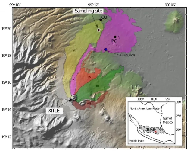
2. Geological setting and sampling 91
The study profile (19.328° N; 99.189° W) is part of the flow VI of Xitle (Fig. 1) located 92
inside the campus of UNAM (Universidad Nacional Autónoma de Mexico). Xitle lies in the 93
central sector of the Trans-Mexican Volcanic Belt (TMVB, Fig. 1) which is an E–W trending 94
zone of ca.1000 km length extending from the Pacific Ocean to the Gulf of Mexico. The 95
TMVB is divided in western, central, and eastern sectors. The Sierra de Chichinautzin 96
Volcanic Field (SCVF) is located in the central sector (inset Fig. 1). 97
The SCVF contains high concentration of monogenetic volcanoes with about 220 Quaternary 98
volcanic products including cinder cones and lava flows (Siebe, 2000; Rodríguez-Trejo et 99
al., 2019) of wide compositional range. Xitle is considered as the youngest monogenetic 100
volcano of the SCVF with a radiocarbon age of 1530-1630 uncalibrated yr BP (cal. 370±60 101
AD; Siebe et al., 2004; Arce et al., 2013). Xitle eruption is an example of the impact of 102
volcanic disaster on the human population, as supposedly it had damaged the pre-Hispanic 103
settlements around Cuicuilco pyramid (Fig. 1) which prompted them to emigrate (Siebe, 104
2000), as like in the historical eruptions of the Jorullo (1759–1774 AD; Guilbaud et al., 2011; 105
Rasoazanamparany et al., 2016; Alva-Valdivia et al., 2019) and Paricutin (1943–1952 AD; 106
Luhr and Simkin, 1993; Pioliet al., 2008) monogenetic volcanoes. 107
The sampled site was selected so that the bottom and top of the lava section (Fig. 3) are 108
visible. Sampling was done using a portable gasoline powered drill, and 72 core samples, 109
each with 5-10 cm long and 2.5 cm diameter, were collected. In this study, four profiles(Fig. 110
3)were taken and distributed as follow: one vertical profile (V) of ca. 4.5 m thickness and 111
composed of 43 cores; and three horizontal profiles (H) of ca.1.25 m length for each: top 112
horizontal (HT) of 11 cores; middle horizontal (HM) of 10 cores; and the bottom horizontal 113
(HB) of 11 cores. 114
3. Previous PI studies 115
Nine PI studies were conducted on Xitle lava flows by means of the double heating Thellier 116
(Nagata et al., 1965; Urrutia-Fucugauchi, 1996; Gonzales et al., 1997; Alva Valdivia, 2005; 117
Böhnel et al., 1997; Morales et al., 2001, 2006; Mahgoub et al., 2019); microwave (Böhnel 118
et al., 2003); and Shaw (Urrutia-Fucugauchi, 1996; Gonzales et al., 1997) methods.Sampling 119
in five of these studies were collected randomly and its coordinates are of low precision 120
which makes us unable to define target flow unit in some of them. On the other hand, three 121
studies (Böhnel et al. , 1997; 2003; Alva-Valdivia et al., 2005) were designed so as to sample 122
vertical profiles over a specific cooling unit. 123
Two studies (Böhnel et al., 2003; Mahgoub et al., 2019) were carried out on pottery fragments 124
that were reheated by Xitle eruption and thus acquired their magnetization at the same time. 125
Böhnel et al. (2003) have performed microwave experiments on lavas and pottery fragments, 126
with the field applied perpendicular and parallel to the their NRMs. We note also that PI data 127
points presented in Böhnel et al. (1997) have been re-analyzed by Böhnel et al. (2003) 128
applying a stringent set of selection criteria. At this point, it must be stated that Böhnel et al. 129
(1997) carried out their study rather to find out how PI varies over the Xitle flow (see section 130
5.2) and if there is a relation between rock magnetic properties and success rate, therefore 131
they have not used a very strict selection criteria. Morales et al. (2006) tried to figure out the 132
cause of PI dispersion through conducting cooling rate correction. Based on their results, a 133
significant decrease in PI-dispersion was obtained (from 7.5 to 3.5 µT), thus they have 134
claimed that cooling-rate effect may have a prominent role in the observed dispersion. There 135
are two points to be mentioned in this context: the first is that Morales et al. (2006) have 136
obtained positive and negative corrections from nearby samples (of 10-20 cm distance) that 137
should have a very similar cooling rate. Secondly, if the change in the cooling rate is the 138
reason for the PI-dispersion, then, reasonably, Thellier results will give less scatter than 139
microwave approach, as the duration of each microwave step is 𝑐𝑎. 10 seconds (Hill and 140
Shaw, 1999). Böhnel et al. (2003), though using microwave technique on a nearby profile, 141
provided PI mean results with similar dispersion as commonly obtained in Thellier. These 142
two points most likely rule out the effect of cooling rate as a major cause of intensity variation 143
acquired from Xitle volcano. 144
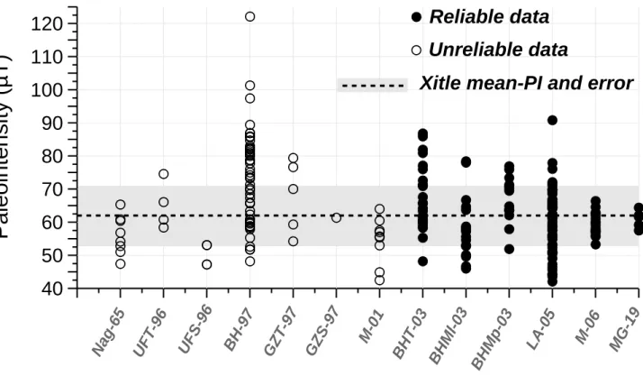
In order to demonstrate the PI mean and scatter in each study and to illustrate the consistency 145
between different studies, we plot the PI data at specimen level on Figure 2. They are 214 146
data points [211 derived from Thellier and microwave and 3 from Shaw method] considered 147
acceptable by the author(s) of each work. As Figure 2 illustrates, the data from each study is 148
highly scattered and the whole data are inconsistent as well. We note that the PI-dispersion 149
of these studies cannot be compared as the number of data is not equal: half of data were 150
obtained by Böhnel et al. (1997) and Alva-Valdivia et al. (2005) while Urrutia-Fucugauchi 151
(1996) and Gonzalez et al. (1997) provided only 3 PI data points using Shaw technique. Using 152
all data, we calculate Xitle PI mean at 64.1 µT (Fig. 2) and the 95% standard deviation (σ) is 153
11 µT, ca. 18% of the mean. Since the number of data is generously available and meet the 154
suggestion of Biggin et al. (2003) that PI mean value of any lava flow should be based on as 155
many samples as possible (at least five). Apparently this dispersion could be related to, 156
among others, some problems in the experimental PI methods (especially those applied long 157
time ago). We evaluate previous 211 Thellier and microwave - derived PI data in terms of 158
recently proposed reliability standards (e.g. Tauxe and Staudigel 2004; Chauvin et al., 2005; 159
Paterson et al., 2014). There are some other problems that could be seriously responsible for 160
such dispersion, including alteration of the ferromagnetic particles, cooling rate effect, and 161
presence of local magnetic field effects. These effects will not be addressed here. 162
Besides the low number of provided data, the two studies that used Shaw experiment 163
(Urrutia-Fucugauchi, 1996; Gonzalez et al.,1997) cannot be considered reliable as they did 164
not perform alteration tests (e.g. Tsunakawa and Shaw, 1994). In Thellier experiments, 165
samples are heated up gradually from low (e.g. 100 °C) to high temperature (commonly 166
below curie point) and the natural remanent magnetization (NRM) is consecutively replaced 167
by laboratory induced thermal remanent magnetization (TRM), in a known laboratory field. 168
This must be done with some alteration checks (Coe et al., 1978) in order to ensure that no 169
alteration occurred during repeated heating. Laboratory procedure of microwave method is 170
the same as Thellier but instead of heating in a conventional oven, samples are demagnetized 171
by exposure to high-frequency microwave (Walton et al., 1993). It has been proved by Hill 172
et al. (2002) that microwave demagnetization is equivalent to thermal counterparts implying 173
that sample’s NRM is replaced by a laboratory induced TRM, for further details we refer to 174
the work of Hill and Shaw (2000) and Böhnel et al. (2003). Due to similarity in experimental 175
approaches, we have set for PI data derived from Thellier and microwave the same criteria 176
set, which are: 177
1) Treated sample must have been checked for thermal alteration during heating by means of 178
the pTRM check criterions (δCK and/or δpal); 179
2) The stability of the sample’s NRM directions during the experiments must have been 180
evaluated by one or all next parameters: MADanc, α, or DANG; 181
3) Following Biggin et al. (2003) suggestion, at least 5 specimens must have been used to 182
compute lava flow mean intensity with σ ≤10 μT or ≤20% of the mean. 183
Applying these criteria set, we found that data presented in the work of Nagata et al. (1965), 184
Urrutia-Fucugauchi (1996), Gonzalez et al. (1997), Böhnel et al. (1997), Morales et al. (2001) 185
do not satisfy the mentioned criteria (Fig. 2). On the other hand, studies of Böhnel et al. 186
(2003), Alva Valdivia (2005), Morales et al. (2006), and Mahgoub et al. (2019) are reliable. 187
We calculate the Xitle mean PI from the 134 data considered as reliable data at 62.0 µT with 188
σ of 9.3 µT (see Fig. 2). This mean value is slightly below the mean calculated from all data 189
and the error is also reduced, however statistically they are indistinguishable at the 95% 190 confidence limit. 191 4. Methods 192
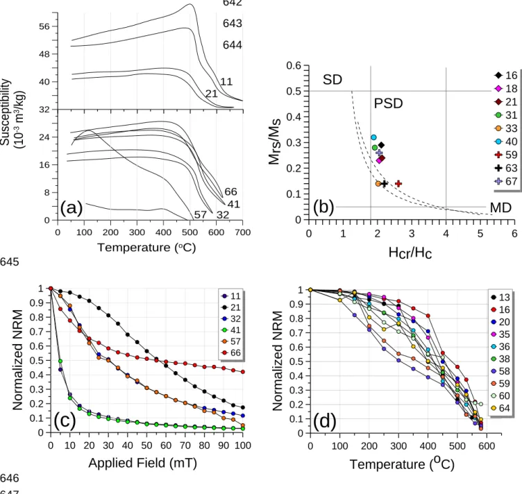
Rock magnetic experiments represented by the susceptibility versus temperature (k-T) 193
analyses and hysteresis measurements were done on 2-3 samples from each sampled profile 194
in order to check the magnetic variability in both horizontal and vertical directions. 195
Alternating field (AFD) and thermal demagnetization (THD) were measured in all the 196
samples of each profile. k-T curves were carried out up to ~700°C with a Bartington-MS2 197
susceptibility-meter coupled with the furnace XXXX (????), and the mean Curie temperature 198
(Tc) were defined as the inflection point after peaks in k. We evaluate the thermal alteration 199
that could occur during the laboratory heating by calculating a reversibility 200
parameter: 𝑅𝑃% =𝑘ℎ−𝑘𝑐
𝑘ℎ ∗ 100; where khand kc represent values of k at heating and cooling
201
curves at 100°C, respectively(reference ??°). Zero RP% indicates that the heated specimen 202
does not experience alteration. Hysteresis analyses were executed with the AGFM 203
(Alternating Gradient Force Magnetometer)for which samples weighting 5 to 40 mg were 204
used. The hysteresis parameters (saturation magnetization (Ms); saturation remanent 205
magnetization (Mrs); coercive force (Hc); and coercivity of remanence (Hcr)) lead to have 206
an idea of the magnetic domain state of the magnetic carriers, Day diagram (Day et al., 1977). 207
AFD measurements were progressively applied from 5 to 100 mT with an AGICO LDA-3 208
equipment. Also, THD was carried out with ASC TD-48 thermal demagnetizer model in 209
every 50 °C from 100 to 500 °C and then from 530 to 600 °C in 30 °C step. From the 210
demagnetization measurements, we have calculated the median destructive field (MDF) and 211
median destructive temperature (MDT), which defined how the alternating field and 212
temperature values of the NRM loses half of its value. 213
PI experiments were estimated with the multispecimen method (Dekkers and Böhnel, 2006) 214
through which specimens are heated only once in different DC fields directed, independently, 215
parallel to the their NRM. The original protocol includes two steps: m0 and m1. Thereafter, 216
two additional steps (m2 and m3) were proposed by Fabian and Leonhardt (2010) in order to 217
correct for the domain state effect, and one more step (m4), where we repeat m1, is proposed 218
to check for any mineralogical alteration occurred during the experiment. In this study, 37 219
specimens were taken from all profiles to conduct the original (MSP-DB; referred to Dekkers 220
and Böhnel) and corrected (MSP-DSC; referred to domain state correction) protocols. 221
Heatings were carried out by use of a new infra-red-heating ultra-fast furnace developed and 222
available in the Geosciences Montpellier laboratory, called ‘FUReMAG’. The heating-223
cooling time in the FUReMAG furnace lasts 45 minutes. Based on the k-T curves and THD 224
results, the set-temperature will be selected so as to ensure unblocking sufficient portion of 225
NRM. Thus, we can get steeped linear fit with small confidence limit (Monster et al., 2015a), 226
and also magneto-mineralogical alteration can be avoided. To eliminate unwanted viscous 227
component in the NRM, the specimens were heated to 100°C and cooled to room temperature 228
in zero field, before the NRM measurement (m0 step). To be consistent with this pre-229
treatment, the low temperature pTRM[100°C,Troom] was removed in the same way after 230
each pTRM acquisition (m1, m2, m3, and m4 steps) involved in the MSP-DSC protocol. The 231
magnetic remanence was measured with a cryogenic magnetometer (2G). 232
5. Results 233
5.1 Magnetic properties
234
The k-T curves (Figs.4a) indicate the presence of several magnetic minerals in distinct 235
proportion. The Tc range from 540 to > 600 °C and RP% from 4 to 80%, suggesting the 236
presence of magnetite (Mag), Ti-poor titanomagnetite (Ti-poor TMag), and hematite with 237
varied reversibility degrees. In all studied samples, k value decrease after heating, indicating 238
that enclosed magnetic minerals have been oxidized. We found that both Tc and RP% do not 239
have any systematic behavior vertically or horizontally, but we can mention that HT and HM 240
profiles have moderate to good reversibility, respectively. Specimens of HB gave dissimilar 241
results and thus no clear conclusion can be outlined. 242
Hysteresis analyses show that all investigated samples are located in the range of PSD field 243
(Fig. 4b), which may suggest presence of a mixture of SD and MD particles in different 244
percentages. HT samples are located close together in the Day plot while those of HM and 245
HB did not show similar consistency. We deduced from these observations that HT profile 246
has a small homogenous PSD particles while, on the other hand, the middle and bottom 247
profiles have somewhat larger ferromagnetic particles of widespread type and/or size. 248
Apparently, few samples are provided this explanation and thus more samples would lead to 249
track better the domain state along vertical and horizontal profiles. However, the recent 250
findings of Roberts et al. (2018) should be mentioned where they find out that domain state 251
of a sample cannot be grasped simply from the Day plot as the hysteresis parameters are 252
based on several variables (Roberts et al., 2018). 253
Intensity-decay curves along the three horizontal profiles results from AFD measurements 254
(Fig. 4c) do not show any systematic behavior (as in previous experiments), and the MDF 255
ranges from 5 to 55 mT thus indicating the presence of varying magnetic grain composition 256
along the three sampled profiles. The THD data (Fig. 4d) showed the appearance of common 257
Tc point of magnetite (ca. 560°C) with small contribution from hematite, thus in agreement 258
with k-T curves. The MDTs are from 300 to 500 °C with a tendency of HB’s samples (58, 259
59 and 64) to have lower MDT in comparison to HT and HM. This tendency could be 260
attributed to the presence of different Ti contents (as they have low unblocking temperature 261
spectra) or to large magnetic minerals size in the HB samples. 262
To sum up, magnetic experiments showed that rock from the sampled profiles, although of 263
limited vertical and horizontal spread, have wide range of type composition and size of the 264
enclosed magnetic minerals. 265
5.2 MSP-DSC results
266
The multispecimen data corrected for domain state (DSC) were analyzed with MSP-267
Tool (Monster et al., 2015) software. The set-temperature throughout the experiments is 268
400°C and applied DC fields range from 10 to 80 µT. The domain state proxy (α-parameter) 269
was set to 0.5, as proposed by Fabian and Leonhardt (2010). Credibility of the MSP results 270
were checked by three parameters: thermal-induced alteration |εalt| parameter (Fabian & 271
Leonhardt 2010; Monster et al. 2015b); the maximum allowed angle (θ) between the isolated 272
NRM and acquired pTRM; and the intersection parameter (∆b) (Monster et al., 2015b), which 273
tests whether the linear fit regression line intersects the y-axis at the theoretically predicted 274
value of −1. In order to confirm the obtained and only reliable results, we have set |εalt| ≤ 275
5%, θ must be less than 10°, and a threshold value of ∆b is ± 0.1. In the MSP-Tool software, 276
the bootstrap statistics were applied to calculate the mean and 95% confidence intervals. 277
Technically, successful MSP experiments were obtained from profiles V and HT, while both 278
HM and HB failed to give reliable estimates as their εalt parameter exceeded the defined 279
limit. In V, three specimens out of nine were rejected (Fig. 5a) as they have altered during 280
the MSP run. The remaining six met the criteria limit defined above and thus a domain state 281
corrected PI mean of 62.9±2.6 µT was obtained for the vertical profile. The HT gave 282
successful MSP experiment in eight out of ten specimens (Fig 5b), with PI value of 58.6 µT, 283
after DSC procedure. We note here that 95% confidence interval in HT (+6.5/-6.3 µT) is 284
almost double the value of the confidence interval in V. Obviously, this high scatter is 285
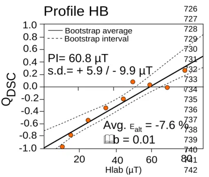
reasoned by the noticeable nonlinearity behavior, in the last field steps (Fig. 5b), between the 286
TRM and applied magnetic field. This non-ideal behavior can be attributed to presence of 287
large ferromagnetic particles, which can reduce the efficiency of linearity law (Selkin et al., 288
2007). Regarding to HM, only one specimen out of nine passed the alteration limit (Fig. 5c), 289
indicating that most of the middle-zone specimens are susceptible to alteration. In addition, 290
the last data points are not aligned linearly which probably point to the dominance of MD 291
particles. Therefore, no reliable results were obtained from this profile. 292
We have neglected the criteria limits to obtain reliable results without regard to data quality, 293
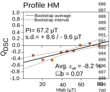
just to see the impact of the sample position in vertical profile on the PI results. A MSP-DSC 294
value of 67.2 µT was obtained, this is demonstrated in the supplementary Figure S1. Three 295
accepted data out of nine (33% success rate) was found along HB profile (Fig. 5d) and thus 296
no meaningful estimate could be obtained. As in HM, if we neglect the criteria set parameters 297
(Fig. S2), a value of 60.8 µT is calculated for HB profile. 298
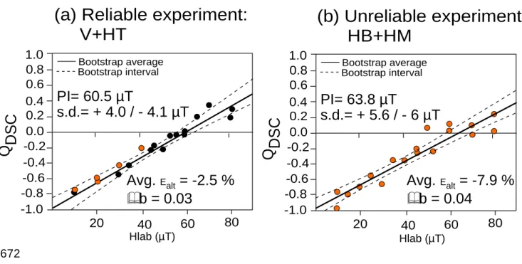
From the above results, it is obvious that only the vertical and upper horizontal profiles gave 299
reliable results that meet the proposed criteria limits. Therefore, combining all accepted 300
specimens from V and HT enables us to assign Xitle-mean PI (Fig. 6a) at 60.5 (+4.0/-4.1) 301
µT. Including all the 18 specimens of HM and HB (Fig. 6b) gives, unexpectedly, a mean
302
value of 63.8 (+5.2/-5.8) µT, which considering the uncertainty limits, isindistinguishable 303
from the mean value calculated from only reliable results.This consistency may denote that 304
the current conditions set for accepting the MSP results (εalt and ∆b) are ineffective. Such 305
explanation, however, cannot be confirmed in this study, as the actual intensity value during 306
Xitle eruption time (370 AD) is unknown. But, we can deduce that obtaining reliable MSP 307
results for a certain lava unit could be achieved by taking many specimens as possible from 308
different parts within the lava flow. However, these approaches will costs effort and time. 309
6. Discussion 310
Three horizontal profiles were sampled from Xitle in three levels from bottom to top in order 311
to discuss horizontal variations of paleointensity. Horizontal characteristics along these 312
profiles were investigated as well through sampling one vertical profile of ca. 4.5 m 313
thickness. Rock magnetic experiments were completed to infer the type and size of the 314
ferromagnetic minerals and their thermal stability. It must be mentioned that the number of 315
present samples that have undergone magnetic experiments and MSP run are few and uneven, 316
and thus the relationship between magnetic properties and paleointensity behavior along 317
lava’s profile may not be clear. However is not the main focus of this study, as we here try 318
to enhance the PI estimates of Xitle by evaluating previous data and conducting a new MSP 319
experiment. Completing this, we can provide an average value with low confidence limit, 320
through combining present PI results with reliable results obtained from previous studies. 321
Despite the limited number of data, we can give a general overview of the impact of lava 322
position and its physical and magnetic properties on the MSP results. Currently, few studies 323
have addressed the relation between rock magnetic properties and lava flow thickness. Some 324
studies (Coe et al., NATURE, 1995; Rolph, 1997; Hill and Shaw, 2000; Vérard et al., 2012) 325
have discussed this relation on thin lava flows, thickness < 2 m, some others extended these 326
studies to thicker lavas of ~6m long (Böhnel et al., 1997; de Groot et al., 2014), and up to 327
several tens of meters (e.g. Wilson et al., 1968; Audunssen et al., 1992). Findings from these 328
studies indicate an effect of the sampling location on the magnetic properties. Lava thickness 329
reflects different cooling history, the top and bottom parts cooled faster than the central part 330
of the flow. These variations in cooling time govern the size of the ferromagnetic crystals 331
and their oxidations states. The top part of the lava flows may produce smaller ferromagnetic 332
sensus lato particles with lower oxidation state in comparison to those formed in the middle 333
of the flow (see for example Böhnel et al., 1997; de Groot et al., 2014). 334
Böhnel et al. (1997) showed detailed results of Xitle’s rock magnetic properties (i.e. Tc, 335
magnetic susceptibility, hysteresis parameters, and coercivities) and PIs along a vertical 336
profile of 6 m thickness. Results indicate that, unlike magnetic properties, the PIs seem to 337
have a systematic behavior with tendency of middle flow samples to give larger PI variations 338
in comparison to the top and bottom samples. Despite the detailed study, they did not find 339
meaningful relation between PI variations and physical and magnetic properties. Our 340
sampled profile spaced only (0.96 km) from Böhnel et al. (1997) profile, implying that they 341
shared almost the same cooling history. The rock-magnetic experiments done in this study 342
showed that Ti-poor TMt and/or Mt is the dominant ferromagnetic mineral(s) and few 343
hematite is present, showed from k-T curves (Fig. 4a). These minerals are located broadly on 344
the PSD size with wide range of MDF ( from ca. 5 to 56 mT). From top to bottom (V), and 345
along each horizontal profile (HT, HM, HB), we do not find any systematic changes on the 346
magnetic properties although of the, above mentioned, differences in cooling times. Although 347
the magnetic parameters obtained in this study varied (e.g. RP%, MDF and MDT) 348
horizontally, we consider that they do not reflect true magnetic properties changes, as the 349
cooling time and content of the cooled lava on such a small scale (1.5 m) are seemingly 350
constant, at least in comparison to vertical direction. This discrepancy in magnetic data could 351
be attributed to the limited number of rock magnetic experiments carried out. In conclusion, 352
there is not a direct connection found between lava thickness and its 1.5 m lateral extent with 353
the magnetic properties. 354
Now, we discuss the influence of cooling time on the MSP results. Our contributed results 355
show that the topmost horizontal profile and the vertical profile have yielded successful MSP-356
DSC PI determinations from the 14 selected samples out of 19 available (74% success rate). 357
On the hand, samples from central and bottom parts of the flow do not give satisfactory MSP 358
results, as they have exceeded the limits of criteria set designed following Monster et al. 359
(2015). Apparently, getting differential MSP results and success rate from over a flow section 360
of 4.5 m thickness can be directly related to the cooling time of this flow. It means that top 361
part of the Xitle flow is appropriate for conducting MSP experiments as it has cooled faster 362
than underlying horizontal sections. Moreover, conducting the experiment vertically does 363
give almost the same results given from HT profile (Fig. 5a and b), which could indicate that 364
the effect of cooling time on MSP results may be insignificant or even disappeared if samples 365
are taken vertically. This explanation is based on a few number of samples and more studies 366
are needed to emphasize it. From these notes, we recommend sampling a lava flow 367
horizontally from its top part when the lava flow is notovered by a younger flow, and 368
vertically in order to give a reliable MSP estimates. 369
370 371
7. Conclusions 372
The rock magnetic properties indicate that the main magnetic minerals are Ti-poor 373
titanomagnetite with small contribution from hematite of PSD carriers accomplish the quality 374
criterion to be able for paleointensity experiments. 375
Successful MSP-DSC experiments were obtained from profiles V and HT, while both HM 376
and HB failed to give reliable estimates. Results obtained in this study from 14 accepted 377
specimens of HT and V profiles give an average mean for Xitle at 60.5 (+4.0/-4.1) µT. This 378
value constrains greatly the dispersion and we consider it should substitute the value for the 379
Xitle from the database used by models in order to do more precise the secular variation 380
curve used for the dating of geologic and archeomagnetic materials of this period. 381
This mean value is consistent with the mean (62.0 ± 9.3 µT) calculated from 134 filtered 382
Thellier & microwave old PI data. The whole PI mean value for Xitle, using a combined 383
formula (Higgins and Green, 2011) gives 61.9 ± 9 µT. This mean value is calculated from 384
high quality data provided from three different PI methods, therefore most likely represents 385
the intensity value for Central Mexico at ca. 370 AD. 386
387 388
Acknowledgments 389
We appreciate the financial support to L. M. Alva-Valdivia from PAPIIT-DGAPA-UNAM 390
IN113117 and ANR-CONACyT (France-Mexico) 273564, research projects. AN Mahgoub 391
acknowledged the financial support of the Universidad Nacional Autónoma de México-392
postdoctoral fellowship. M. A. Bravo-Ayala was partly financially supported by a 393
scholarship from CONACyT and a Research Grant from Dr. P. Camps and Dr. T. Poidrás 394
whom allowed the use of the Paleomagnetic laboratory of Geoscience University of 395
Montpellier, France. Thanks to J. A. González Rangel for the support on the Mexican 396
Paleomagnetic laboratory experiments. 397
398 399 400 401
402
References 403
Aitken, M., Allsop, A., Bussell, G., Winter, M., 1988. Determination of the intensity of the 404
Earth’s magnetic field during archaeological times: Reliability of the Thellier 405
technique. Rev. Geophys. 26 (1), 3–12. 406
Alva-Valdivia, L., 2005, Comprehensive paleomagnetic study of a succession of Holocene 407
olivine-basalt flow: Xitle Volcano (Mexico) revisited, Earth Planets Space, Vol. 57, 408
pp. 869-853. 409
Audunssen, H., S. Levi, and F. Hodges (1992), Magnetic property zonation in a thick lava 410
flow, J. Geophys. Res., 97(B4), 4349–4360. 411
Biggin, A.J., Steinberger, B., Aubert, J., Suttie, N., Holme, R., Torsvik, T.H., van der Meer, 412
D.G., van Hinsbergen, D.J.J. (2012) Possible links between long-term geomagnetic 413
644 variations and whole-mantle convection processes. Nat Geosci 5:526–533 414
Biggin, A.J., Böhnel, H.N. & Zuniga, F.R., 2003. How many paleointensity determinations 415
are required from a single lava flow to constitute a reliable average? Geophys. Res. 416
Lett., 30(11). 417
Böhnel, H., Morales, J., Caballero, C., Alva, L., McIntosh, G., González, S. y Sherwood, J., 418
1997, Variation of rock magnetic parameters and paleointensities over a single 419
holocene lava flow, J. Geomag. Geoelectr., 49, 523 - 542. 420
Böhnel, H., E. Herrero-Bervera, and M. J. Dekkers (2011), Paleointensities of the Hawaii 421
1955 and 1960 Lava Flows: Further Validation of the Multi-specimen Method, pp. 422
195–211, Springer, Dordrecht, Netherlands. 423
Böhnel, H., A. J. Biggin, D. Walton, J. Shaw, and J. A. Share (2003), Microwave 424
palaeointensities from a recent Mexican lava flow, baked sediments and reheated 425
pottery, Earth Planet. Sci. Lett., 214, 221–236. 426
Coe, R.S., 1967. Paleo-intensities of the Earth's magnetic field determined from Tertiary 427
and Quaternary rocks. J. Geophys. Res. 72 (12), 3247–3262. 428
Coe RS, Grommé S, Mankinen EA (1978) Geomagnetic paleointensities from radiocarbon 429
dated lava flows on Hawaii and the question of the Pacific nondipole low. J Geophys 430
Res Solid Earth 83(B4):1740–1756 431
Cromwell, G., Tauxe, L., Staudigel, H., Ron, H., 2015. PI estimates from historic and 432
modern Hawaiian lava flows using glassy basalt as a primary source material. 433
Phys. Earth Planet. Inter.241, 44–56. 434
de Groot, L. V., T. A. T. Mullender, and M. J. Dekkers (2013), An evaluation of the influence 435
of the experimental cooling rate along with other thermomagnetic effects to explain 436
anomalously low palaeointensities obtained for historic lavas of Mt Etna (Italy), 437
Geophys. J. Int., 193(3), 1198–1215, doi:10.1093/gji/ggt065. 438
de Groot, L.V., Dekkers, M.J., Visscher, M., ter Maat, G.W., 2014. Magnetic properties and 439
paleointensities as function of depth in a Hawaiian lava flow. Geochem. Geophys. 440
Geosyst.15. http://dx.doi.org/10.1002/2013GC005094. 441
Day, R., Fuller, M., Schmidt, V.A., 1977. Hysteresis properties of titanomagnetites: grain 442
size and compositional dependence. Phys. Earth Planet. Inter. 13, 260–267. 443
Dekkers, M.J., Böhnel, H.N., 2006. Reliable absolute palaeointensities independent of 444
magnetic domain state. Earth Planet. Sci. Lett. 284, 508-517. 445
Dunlop, D.J., 2002. Theory and application of the Day plot (Mrs/Ms versus Hcr/Hc) 1. 446
Theoretical curves and tests using titanomagnetite data. J. Geophys. Res 107(B3) 447
2056. doi:10.1029/2001JB000486. 448
Fabian, K., Leonhardt, R., 2010. Multiple-specimen absolute PI determination: An optimal 449
protocol including pTRM normalization, domain-state correction, and alteration test. 450
Earth Planet. Sci. Lett. 297, 84–94. 451
Gonzalez S, Sherwood GJ, Boehnel H, Schnepp E (1997), Paleosecular variation in central 452
Mexico over the last 30,000 years: The record from lavas. Geophys J Int 130: 453
201− 219. 454
González, S., Pastrana, A., Siebe, C., Duller, G., 2000. Timing of the prehistoric eruption of 455
Xitle volcano and the abandonment of Cuicuilco pyramid, southern Basin of Mexico. 456
Geol. Soc. London Sp. Pub. 171, 205-224.
457
https://doi.org/10.1144/GSL.SP.2000.171.01.17. 458
Grappone, J.M., Biggin, A.J., Hill. M.J., 2019: Solving the mystery of the 1960 Hawaiian 459
lava flow: implications for estimating Earth’s magnetic field. Geophys. J. Int., 218, 460
1796–1806. 461
Guilbaud, M.N., Siebe, C., Layer, P., Salinas, S., 2012. Reconstruction of the volcanic history 462
of the Tacámbaro-Puruarán area (Michoacán, México) reveals high frequency of 463
Holocene monogenetic eruptions. Bull. Volcanol. 74, 1187–1211. 464
465
Heizer, R.F., Bennyhoff, J.A., 1958. Archeological investigations of Cuicuilco, Valley of 466
Mexico, 1957. Science 127, 232±233. 467
Higgins J and Green S. Cochrane Handbook for Systematic Reviews of Interventions 468
Version 5.1.0. The Cochrane Collaboration, 2011, www.handbook.cochrane.org.
469
Hill, M. J., and J. Shaw (1999), Palaeointensity results for historic lavas from Mt Etna using 470
microwave demagnetization/remagnetization in a modified Thellier-type 471
experiment, Geophys. J. Int., 139(2), 583–590 472
Hill, M. J., and J. Shaw (2000), Magnetic field intensity study of the 1960 Kilauea lava flow, 473
Hawaii, using the microwave PI technique, Geophys. J. Int., 142, 487–504. 474
Luhr, J.F., Simkin, T., 1993. Paricutin: The Volcano Born in a Mexican Cornfield. 475
Geoscience Press (427 p). 476
Mahgoub, A.N., Juárez-Arriaga, E., Böhnel, H., Manzanilla, L.R., Cyphers, A., 2019. 477
Refined 3600 years palaeointensity curve for Mexico. Phys. Earth Planet. Inter. 478
Accepted. 479
Morales, J., Alva-Valdivia, L., Goguitchaichvili, A. y Urrutia-Fucugauchi, J., 2006, Cooling 480
rate corrected paleointensities from the Xitle lava flow: Evaluation of within-site 481
scatter for single spot-reading cooling units, Earth Planets Space, Vol. 58, pp. 1341-482
1347. 483
Morales, J., Goguitchaichvili, A. y Urrutia-Fucugauchi, J., 2001, A rock-magnetic and PI 484
study of some Mexican volcanic lava flows during the Latest Pleistocene to the 485
Holocene, Earth Planets Space, Vol. 53, pp. 893–902. 486
Monster, M.W.L., de Groot, L.V., Biggin, A.J., Dekkers, M.J., 2015a. The performance of 487
various PI techniques as a function of rock magnetic behaviour – a case study for 488
La Palma. Phys. Earth Planet. Inter. 242, 36–49. http://dx.doi.org/10.1016/ 489
j.pepi.2015.03.004 490
Monster, M.W.L., de Groot, L.V., Dekkers, M.J., 2015b. MSP-tool: a VBA-based software 491
tool for the analysis of multispecimen PI data. Front. Earth Sci. 3, 86. 492
http://dx.doi.org/10.3389/feart.2015.00086. 493
Nagata, T., Kobayashi, K., Schwarz, E.J., 1965. Archaeomagnetic intensity studies of South 494
and Central America. J. Geomagnetism Geoelectricity, 17, 399-405, 495
https://doi.org/10.5636/jgg.17.399 496
497
Nilsson A, Holme R, Korte M, Suttie N, Hill M (2014) Reconstructing Holocene 498
geomagnetic field variation: New methods, models and implications. Geophys J Int 499
198(1):229–248 500
Paterson GA, Tauxe L, Biggin AJ, Shaar R, Jonestrask LC (2014) On improving the 843 501
selection of Thellier-type paleointensity data. Geochem Geophys Geosyst 15(4): 502
1180–844 1192 503
Paterson, G. A., L. Tauxe, A. J. Biggin, R.Shaar, and L. C. Jonestrask (2014), On improving 504
the selection of Thellier-type paleointensity data, Geochem.Geophys. Geosyst., 15, 505
1180–1192,doi:10.1002/2013GC005135. 506
Pavón-Carrasco, F.J., Osete, M.L., Torta, J.M., De Santis, A., 2014. A geomagnetic field 507
model for the Holocene based on archaeomagnetic and lava flow data. Earth Planet. 508
Sci. Lett. 388, 98–109. 509
Pioli, L., Erlund, E., Johnson, E., Cashman, K.V., Wallace, P., Rosi, M., Delgado, H., 2008. 510
Explosive dynamics of violent Strombolian eruptions: the eruption of Paricutin 511
volcano 1943–1952 (Mexico). Earth Planet. Sci. Lett. 271 (1–4), 359–368. 512
Rasoazanamparany, C., Widom, E., Siebe, C., Guilbaud, M.-N., Spicuzza, M.J., Valley, J.W., 513
Valdez, G., Salinas, S., 2016. Temporal and compositional evolution of Jorullo 514
volcano, Mexico: implications for magmatic processes associated with a 515
monogenetic eruption. Chem. Geol. 434, 62–80. 516
Rolph, T.C., 1997. An investigation of the magnetic variation within two recent lava flows, 517
Geophys. J. Int., 130, 125–136. 518
Roberts, A.P., Tauxe, L., Heslop, D., Zhao, X., Jiang, Z., 2018. A critical appraisal of the 519
Day diagram. J. Geophys. Res. 123, 2618–2644. 520
https://doi.org/10.1002/2017JB015247. 521
Selkin, P. A., J. S. Gee, and L. Tauxe (2007), Nonlinear thermoremanence acquisition and 522
implications for PI data, Earth Planet. Sci. Lett., 256, 81–89, 523
doi:10.1016/j.epsl.2007.01.017. 524
Siebe, C., 2000. Age and archaeological implications of Xitle volcano, southwestern Basin 525
of Mexico-City. J. Volcanol. Geotherm. Res. 104, 45-64. 526
https://doi.org/10.1016/S0377-0273(00)00199-2. 527
Shaw, J., 1974, A new method of determining the magnitude of the paleomagnetic field 528
application to 5 historic lavas and five archeological samples. Geophysical Journal 529
of the Royal Astronomical Society 39: 133-141. doi: 10.1111/j.1365-530
246X.1974.tb05443.x. 531
Stacey, F.D. & Banerjee, S.K., 1974. The Physical Principles of Rock Magnetism, Elsevier, 532
Amsterdam. 533
534
Tauxe, L., T. Pick, and Y. Kok (1995), Relative PI in sediments: A pseudo-Thellier approach, 535
Geophys. Res. Lett., 22(21), 2885–2888. 536
Thellier, E. & Thellier, O., 1959. Sur l’intensité du champ magnétique terrestre dans le 537
passé historique et géologique, Ann Géophys., 15, 285–376. 538
Tauxe, L., Staudigel, H., 2004. Strength of the geomagnetic field in the Cretaceous Normal 539
Superchron: new data from submarine basaltic glass of the Troodos Ophiolite. 540
Geochem. Geophys. Geosyst. 5 (Q02H06). 541
Tsunakawa, H., Shaw, J., 1994. The Shaw method of PI determinations and its application to 542
recent volcanic rocks. Geophys. J. Int. 118, 781–787. 543
Urrutia Fucugauchi, J., 1996. Palaeomagnetic study of the Xitle- Pedregal de San Angel lava 544
flow, southern Basin of Mexico. Physics of the Earth and Planetary Interiors 97, 177-545
196. 546
Verard, C., R. Leonhardt, and M. Winklhofer (2012), Variations of magnetic properties in 547
thin lava flow profiles: Implications for the recording of the Laschamp Excursion, 548
Phys. Earth Planet. Inter., 200–201, 10–27, doi:10.1016/j.pepi.2012.03.012. 549
Walton, D., Share, J.A., Rolph, T.C. & Shaw, J., 1993. Microwave magnetisation, Geophys. 550
Res. Lett., 20, 109–111. 551
Wilson, R. L., S. E. Haggerty, and N. D. Watkins (1968), Variation of palaeomagnetic 552
stability and other parameters in a vertical traverse of a single Icelandic lava, 553
Geophys. J. R. Astron. Soc., 16, 79–96. 554
Yamamoto,Y., Tsunakawa,H.&Shibuya, H., 2003. Palaeointensity study of the Hawaiian 555
1960 lava: implications for possible causes of erroneously high intensities, Geophys. 556 J. Int., 153(1), 263–276. 557 558 559 560 List of Figures 561 562
Figure 1. Distribution of Xitle lava flows I to VI, with the location of the sampling site and 563
the Cuicuilco archeological site. Modified after Delgado et al. (1998). 564
Figure 2. Evaluation of previous PI data published for Xitle. The closed and open circles 565
represent reliable and unreliable data based on a set of selection criteria designed in this study 566
(see section 2). The dotted line and shaded area is the Xitle mean paleointensity value and 567
95% standard deviation, calculated from only reliable data. the x-axis represent different 568
studies that were done on Xitle. 569
for abbreviations: Nag-65 is Nagata et al. (1965); UFT-96 is Urrutia-Fucugauchi (1996), 570
from thellier experiment; UFS-96 is Urrutia-Fucugauchi (1996) from Shaw experiment; BH-571
97 is Böhnel et al. (1997); GZT-97 is Gonzales et al. (1997) from thellier; GZS-97 is Gonzales
572
et al. (1997) from Shaw; M-01 is Morales et al. (2001); BHT-03 is Böhnel et al. (2003) from 573
thellier after re-analyzing data of Böhnel et al. (1997); BHMl-03 is Böhnel et al. (2003) from 574
microwave done on lavas; BHMp-03 is Böhnel et al. (2003) from microwave done on 575
potteries; LA-05 is Alva-Valdivia (2005); M-06 is Morales et al. (2006); and MG-19 is 576
Mahgoub et al. (2019, accepted for publication). 577
578
Figure 3. Sampling profile. Lava flow with scale (1m). Three zones are observed with the 579
naked eye: the massive central zone and the upper zone that present abundant vesicles and 580
lower with much less and tiny vesicles. The core numbers are shown in order to be compared 581
with upcoming rock magnetic properties and paleointensities. 582
583
Figure 4. Rock magnetic results done in this study: (a) susceptibility vs. temperature curves; 584
(b) Day plot (Day et al., 1977) with thresholds for single domain (SD), pseudo single domain 585
(PSD), and multidomain (MD) shown as straight grey lines. Dashed curved lines represent 586
the SD-MD theoretical mixing curves, after Dunlop (2002); (c) intensity decay curves 587
obtained after alternating field demagnetization; (d) intensity decay curves after thermal 588
demagnetization. Numbers in each panel diagram represent core sample, see Figure 3. 589
AHMED, LAS CURVAS EN 4A CASI NO SE VEN. Y EN 4C Y 4D EL EJE Y DEBE SER 590
NORMALIZED MAGNETIZATION. 591
592
Figure 5. Multispecimen results obtained from four sampled profiles, after domain state 593
correction (DSC). In each DSC protocol, the average alteration parameter (εalt) and the 594
intersection criterion (Δb) are demonstrated to judge the credibility of the given results. Note 595
that data were analyzed with MSP-Tool software (Monster et al., 2015b) where bootstrap 596
statistics were applied to calculate the mean (solid black line) and 95% confidence interval 597
(dashed black lines lines). Black and orange circles represent those accepted and unaccepted 598
data, respectively, based on the criteria limit defined in the present study. (a and b) represent 599
accepted experiments done on profiles V and HT, as their specimens meet the designed 600
criteria limit, and (c and d) represent unaccepted experiments from profiles HM and HB and 601
thus no PI mean could be calculated from these two profiles. 602
603
Figure 6. (a) Xitle PI mean value calculated from only reliable experiments done on V and 604
HT profiles. (b) represents unreliable experiments (from profiles HM and HB), and the 605
bootstrap mean (solid black line) and 95% confidence interval (dashed black lines lines) are 606
shown to compare the Pi results obtained from reliable (a) and unreliable (b) data. 607
608 609
610 611
Figure 1. Distribution of Xitle lava flows I to VI, with location of the sampling site and 612
Cuicuilco archeological site. Modified after Delgado et al. (1998). WE ARE STILL 613
WORKING ON THIS FIGURE! 614 615 616 617 618 619
620 621 622
Figure 2. Evaluation of previous PI data published for Xitle. The closed and open circles 623
represent reliable and unreliable data based on a set of selection criteria designed in this study 624
(see section 2). The dotted line and shaded area is the Xitle mean paleointensity value and 625
95% standard deviation, calculated from only reliable data. the x-axis represent different 626
studies that were done on Xitle. 627
for abbreviations: Nag-65 is Nagata et al. (1965); UFT-96 is Urrutia-Fucugauchi (1996), 628
from thellier experiment; UFS-96 is Urrutia-Fucugauchi (1996) from Shaw experiment; BH-629
97 is Böhnel et al. (1997); GZT-97 is Gonzales et al. (1997) from thellier; GZS-97 is Gonzales
630
et al. (1997) from Shaw; M-01 is Morales et al. (2001); BHT-03 is Böhnel et al. (2003) from 631
thellier after re-analyzing data of Böhnel et al. (1997); BHMl-03 is Böhnel et al. (2003) from 632
microwave done on lavas; BHMp-03 is Böhnel et al. (2003) from microwave done on 633
potteries; LA-05 is Alva-Valdivia (2005); M-06 is Morales et al. (2006); and MG-19 is 634
Mahgoub et al. (2019, accepted for publication). 635 0 1 2 3 4 5 6 7 8 9 10 11 12 13
40
50
60
70
80
90
100
110
120
P
a
le
o
in
te
n
s
it
y
(
µ
T
)
Na g-6 5 UF T-9 6 UF S-9 6 BH -97 GZ T-9 7 GZ S-9 7 M-0 1 BH T-0 3 BH M l-03 BH Mp -03 LA -05 M-0 6 MG -19Unreliable data
Reliable data
Figure 3. Sampling profile. Lava flow with scale (1m). Three zones are observed with the 637
naked eye: the massive central zone and the upper and lower zones that present vesicles. The 638
core numbers are shown in order to be compared with upcoming rock magnetic properties 639
and paleointensities. 640
642 643 644 645 646 647
Figure 4. Rock magnetic results done in this study: (a) susceptibility vs. temperature curves; 648
(b) Day plot (Day et al., 1977) with thresholds for single domain (SD), pseudo single domain 649
(PSD), and multidomain (MD) shown as straight grey lines. Dashed curved lines represent 650
the SD-MD theoretical mixing curves, after Dunlop (2002); (c) intensity decay curves 651
obtained after alternating field demagnetization; (d) intensity decay curves after thermal 652
demagnetization. Numbers in each panel diagram represent core sample, see Figure 3. 653 654 0 100 200 300 400 500 600 700 Temperature (oC) 0 8 16 24 32 40 48 56 S u sc e p tib ili ty ( 1 0 -3 m 3 /k g ) 66
(a)
21 57 11 32 41 0 10 20 30 40 50 60 70 80 90 100 Applied Field (mT) 0 0.1 0.2 0.3 0.4 0.5 0.6 0.7 0.8 0.9 1 N o rm a liz e d N R M 11 21 32 41 57 66(c)
0 100 200 300 400 500 600 Temperature (oC) 0 0.1 0.2 0.3 0.4 0.5 0.6 0.7 0.8 0.9 1 N o rm a liz e d N R M 13 16 20 35 36 38 58 59 60 64(d)
0 1 2 3 4 5 6Hcr/Hc
0 0.1 0.2 0.3 0.4 0.5 0.6M
rs
/M
s
16 18 21 31 33 40 59 63 67SD
PSD
MD
(b)
655 656 657 658 659
Figure 5. Multispecimen results obtained from four sampled profiles, after domain state 660
correction (DSC). In each DSC protocol, the average alteration parameter (εalt) and the 661
intersection criterion (Δb) are demonstrated to judge the credibility of the given results. Note 662
that data were analyzed with MSP-Tool software (Monster et al., 2015b) where bootstrap 663
statistics were applied to calculate the mean (solid black line) and 95% confidence interval 664
(dashed black lines lines). Black and orange circles represent those accepted and unaccepted 665
data, respectively, based on the criteria limit defined in the present study. (a and b) represent 666
accepted experiments done on profiles V and HT, as their specimens meet the designed 667 Q D S C PI= 62.9 µT s.d.= + 2.6 / - 2.6 µT Bootstrap average Bootstrap interval -1.0 -0.8 -0.6 -0.4 -0.2 0.0 0.2 0.4 0.6 0.8 1.0
(a) profile V
20 40 60 80 Hlab (µT) Q D S C PI= 58.6 µT s.d.= + 6.5 / - 6.3 µT Bootstrap average Bootstrap interval -1.0 -0.8 -0.6 -0.4 -0.2 0.0 0.2 0.4 0.6 0.8 1.0 20 40 60 80 Hlab (µT) Avg. Ealt = -2.8 % b = -0.03 Avg. Ealt = -2.3 % b = -0.09(b) profile HT
Q D S C PI = null s.d= null -1.0 -0.8 -0.6 -0.4 -0.2 0.0 0.2 0.4 0.6 0.8 1.0 20 40 60 80 Hlab (µT)(c) profile HM
Q D S C PI = null s.d= null -1.0 -0.8 -0.6 -0.4 -0.2 0.0 0.2 0.4 0.6 0.8 1.0 20 40 60 80 Hlab (µT)(d) profile HB
criteria limit, and (c and d) represent unaccepted experiments from profiles HM and HB and 668
thus no PI mean could be calculated from these two profiles. 669
671
672 673 674 675
Figure 6. (a) Xitle PI mean value calculated from only reliable experiments done on V and 676
HT profiles. (b) represents unreliable experiments (from profiles HM and HB), and the 677
bootstrap mean (solid black line) and 95% confidence interval (dashed black lines lines) are 678
shown to compare the Pi results obtained from reliable (a) and unreliable (b) data 679 680 681
Q
D
S
C
PI= 60.5 µT
s.d.= + 4.0 / - 4.1 µT
Bootstrap average Bootstrap interval -1.0 -0.8 -0.6 -0.4 -0.2 0.0 0.2 0.4 0.6 0.8 1.0(a) Reliable experiment:
V+HT
20 40 60 80 Hlab (µT)Q
D
S
C
PI= 63.8 µT
s.d.= + 5.6 / - 6 µT
Bootstrap average Bootstrap interval -1.0 -0.8 -0.6 -0.4 -0.2 0.0 0.2 0.4 0.6 0.8 1.0 20 40 60 80 Hlab (µT)Avg.
Ealt= -2.5 %
b = 0.03
(b) Unreliable experiment:
HB+HM
Avg.
Ealt= -7.9 %
b = 0.04
Supplementary Materials 682
683
The supplementary materials consist of two figures. 684
685 686 687 688 689 690 691 692 693 694 695 696 697 698 699 700 701
Figure S1. Multispecimen results obtained from central profile (HM), after domain state 702
correction (DSC). The data were analyzed with MSP-Tool software (Monster et al., 2015b) 703
where bootstrap statistics were applied to calculate the mean (solid black line) and 95% 704
confidence interval (dashed black lines lines). We note that in this profile we do not apply 705
the selection criteria defined in the present study, as we just need to compare the unreliable 706
data with reliable data. 707 708 709 710 711 712 713 714 715 716 717 718 719 720 721 722 723 724
Q
D
S
C
PI= 67.2 µT
s.d.= + 8.6 / - 9.6 µT
Bootstrap average Bootstrap interval-1.0
-0.8
-0.6
-0.4
-0.2
0.0
0.2
0.4
0.6
0.8
1.0
Profile HM
20
40
60
80
Hlab (µT)Avg.
Ealt= -8.2 %
b = 0.07
725 726 727 728 729 730 731 732 733 734 735 736 737 738 739 740 741 742 743
Figure S2. Multispecimen results obtained from bottom profile (HB). For details see Fig. 744 S2 caption. 745 746 747