Study and modeling of vibration sources and turbulence in telecommunications systems based on laser satellites.

(1)

République Algérienne Démocratique et Populaire

Ministère de l’Enseignement Supérieur et de la Recherche Scientifique

Université Batna 2 – Mostefa Ben Boulaïd

Faculté de Technologie

Département d’Electronique

Thèse

Présentée pour l’obtention du diplôme de :

Doctorat en Sciences en Electronique

Option : Micro-ondes

Sous le Thème :

Study and modeling of vibration sources and turbulence in

telecommunications systems based on laser satellites.

Présentée par :

Al-Gobi Mohammed Senan Rageh

Devant le jury composé de :

M. FORTAKI Tarek Prof. Université de Batna 2 Président

M. BENATIA Djamel Prof. Université de Batna 2 Rapporteur

M. BOULAKROUNE M’Hamed Prof. ENP Constantine Examinateur

M. BENABDELKADER Souad MCA Université de Batna 2 Examinateur

M. BENSLAMA Malek Prof. Université de Constantine 1 Examinateur

M. BEDRA Sami MCA Université de Khenchela Examinateur

(2)

ركش

لا ةحصلاو ربصلاو ةدارلإا يناطعأ يذلا ميظعلا للها ركشأ نأ دوأ ، ءدب يذ ئداب

زاجن

لمعلا اذه

.

، يل هسرك يذلا تقولاو ةدعاسملا ىلع ةيطع نب لامج روسيفوربلا يفرشمل ركشلاب مدقتأ نأ دوأ

.ًادبأ رونلا ىرتل ةلاسرلا هذه نكت مل هنودبو

ليزجلا ركشلاب هجوتأ

ل

ةسائرب يل همدق يذلا فرشلا ىلع يقاطرف قراط روسيفوربل

نجل

ملا ة

قان

ةش

.

ا : نم لكب ةلثمتملا ةشقانملا ةنجل ءاضعأ اضيأ ركشا نأ دوأ

روسيفوربل

دمحم نورقلوب

نم

، ةنيطنسق ةعماج

و

كلام ةملاس نب روسيفوربلا

نم

ةنيطنسق ةعماج

1 ةعماجب رضاحم ذاتسأ داعس ردا قلا دبع نب و ،

ةنتاب

2 ىلع مهتقفاومل ةلشنخ ةعماجب رضاحم ذاتسأ يماس ةردب و ،

ييقت

.لمعلا اذه م

نع برعأ

صخاو رونلا ىلا لمعلا اذه جارخا يف مهاس و يندعاس نم لكل يريدقتو ينانتما قئا ف

ق يف ذاتسأ ذاعم يلاب ذاتسلأاو ةركسب ةعماجب ةيزيلجنلإا مسق يف ذاتسأ دباعلا رصان ذاتسلأا ركذلاب

مس

.داولا ةعماجب يللاا ملاعلاا

ذه زهتنا امك

نميلا نم ةذتاسلأا يتوخا ىلا ركشلاب مدقتلا ةصرفلا ه

و

مهنم صخا

للهادبع ذاتسلأا

لكوتملا

د

لا مسقب ةاروتكد يسبكلا ميهاربإ ذاتسلأاو ةركسب ةعماجب يلا ملاعا ةراوتك

م

ةعماجب كيناكي

لاا يف ةاروتكد راصعملا لامك ذاتسلأاو ةنتاب

شن

ةركسب ةعماجب تاءا

يف يل مهمعدو ةلاعفلا مهتمهاسمل

نع برعا امك .باعصلاو فورظلا كلحا

لاا عيمجل ينانتما

ةذتاس

ًادهج اورخدي مل نيذلا

ل قصو انريوطتل

.انتاراهم

، اًريخأ

ةفاسملا دعب نم مغرلا ىلع

نع برعأ .نميلا يف نيميقملا يتلئاع دارفأ عيمجل ةصاخ ةناكمب ظفتحا

قيمع

لامكتسلا مهعيجشتو يونعملا مهمعدب ، رارمتساب ينودعاس مهنلأ مهل ينانتما

لا اذه

لمع

.

(3)

ءادـــــــــــــــها

نيزيزعلا يدلاو حور لىا

,

يلافطو يتجوز لىا

,,

يتوخا لىا

,,, يتخا و

نطو لي دعي ملف رئازلجا ينطو لىا

,,,,

عضاوتلما لمعلا اذه يدهأ

(4)

Table of Contenants

Table of contenants

List of Figures ... 4

General introduction ... 5

1 General Overview of satellite communications ... 9

1.1 Introduction ... 9

1.2 Description of satellite communication system ... 9

Ground Sector ... 10

Space Sector ... 10

1.3 Orbits Tracked by Satellites ... 14

Circular orbits ... 15

Elliptical orbit ... 16

1.4 Satellite constellations ... 17

Low Earth Orbit Constellation ... 17

Medium Earth Orbit constellations ... 18

GEO Constellation ... 18

1.5 Geometry between earth and satellite ... 19

1.6 Basics of space mechanics ... 20

Kepler's laws ... 21

Orbital parameters ... 22

Orbital perturbations ... 25

Maintenance and survival in orbit ... 27

1.7 Conclusion ... 28

2 Optical telecommunications and the effect of atmosphere ... 30

2.1 History of optical telecommunications ... 30

2.2 Principle and characteristics of atmospheric optical links ... 33

Modulation of AOLs endo-atmospheric ... 34

Benefits of AOLs endo-atmospheric... 35

The limitations in atmospheric optical links ... 36

2.3 Atmospheric turbulence ... 36

The physical phenomenon of turbulence ... 36

Theory of energy cascades ... 37

The refractive index of air ... 39

(5)

2

Helmholtz equation ... 41

Paraxial approximation ... 42

Weak fluctuations Rytov approximation ... 42

Statistic properties of the field ... 43

Power spectral densities ... 44

Probability density function ... 44

2.5 Effects of turbulence on laser propagation ... 45

Atmospheric turbulence on the Gaussian beam waves ... 45

Impact of Scintillation on propagation ... 47

3 Adaptive Optics for Laser Satellite-To-Ground Communication ... 54

3.2 Adaptive Optics Systems ... 54

Principal components of adaptive optics ... 56

The wavefront analysis ... 57

Modal analysis of the turbulent phase ... 61

3.3 Optimization of adaptive optics system with a free wavefront sensor ... 63

Sensor-less stochastic technique ... 64

Different stochastic parallel optimization algorithms ... 64

3.4 Simulation tools for OA ... 68

OKOTECH ... 69

SCILAB ... 69

Object Oriented Matlab for Adaptive Optics (OOMAO): ... 69

4 Correction wavefront sensor based on stochastic technique for satellite-to-ground laser communication links ... 78

4.2 The SHWF and OOMAO closed-loop technique ... 79

The Shack Hartmann ... 79

OOMAO closed-loop ... 80

4.3 Stochastic technique (genetic algorithm) ... 84

Modeling the problem ... 84

Algorithm flow-chart ... 85

Experimental setup ... 86

(6)

Results of simulation ... 88

4.4 Hybrid GA solution ... 91

Principle of HGA solution ... 91

The flow-chart of HGA solution ... 91

Comparison between OOMAO and Hybrid Algorithm ... 92

4.5 Conclusion ... 92

General Conclusion ... 94

Future work ... 96

(7)

List of Figures

4

List of Figures

Figure 1-1: A component of satellite communication system. ... 10

Figure 1-2: Satellite structure [12]. ... 13

Figure 1-3: Circular orbits. ... 16

Figure 1-4: Elliptical orbit. ... 16

Figure 1-5: GEO constellation. ... 19

Figure 1-6: Geometry between earth and satellite. ... 19

Figure 1-7: Nadir angle and elevation angle. ... 20

Figure 1-8: The ellipse. ... 21

Figure 1-9: Law of areas. ... 21

Figure 1-10: Two-body problem. ... 22

Figure 1-11: Position of the orbit plane. ... 23

Figure 1-12: Classification of the different types of exploitable orbits. ... 28

Figure 2-1 :Optical telegraph of Mangin [27]. ... 31

Figure 2-2: Schematic representation of Graham Bell's photo phone [27]. Under the influence of speech, the mirror deforms and modulates the intensity of the light coming from the sun as it reaches the receiver. The resistance of the selenium receiver varies according to the intensity of the light received and allows the information to be retrieved. ... 31

Figure 2-3: A modern optical telegraph ... 34

Figure 2-4:An overview of the principle of energy cascade in a fluid in turbulent flow where the transfer is from large to small scale[47]. ... 37

Figure 2-5: Schema of the energy cascade process and the division of turbulence cells in the atmosphere. .. 38

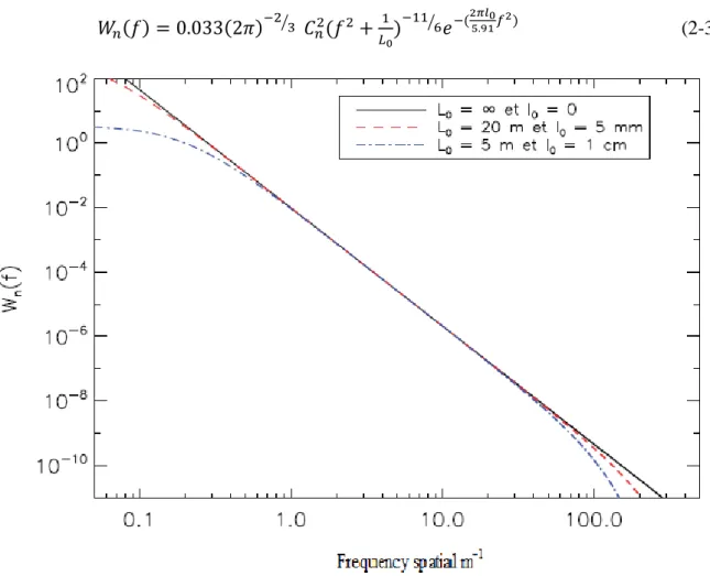
Figure 2-6: Power spectral density of refractive index fluctuations for 𝑪𝒏𝟐𝒉 = 𝟏and different values of inner scale and outer scale. ... 40

Figure 2-7: Propagation of a converging Gaussian beam (radius of curvature> 0 at the origin) in free space without turbulence. ... 47

Figure 2-8: The beam wander effect ... 48

Figure 2-9: Illustration of the impact of atmospheric turbulence on laser propagation in the detection plane. Each footprint corresponds to an independent realization of turbulence. ... 49

Figure 3-1: principle of an AO system in a laser communication application ... 55

Figure 3-2: Actuator layout of two deformable mirrors (left: BMC140 from Boston Micro machines, 140 actuators, segmented/continuous; right: OKO37 from Flexible Optical, 37actuators, continuous) with the typical optical pupil superimposed (from [81]). ... 56

Figure 3-3: principle of an AO system in a laser communication application ... 57

Figure 3-4: The Shack-Hartmann analyzer wave surface analyzer... 58

Figure 3-5: The first 21 Zernike polynomials ordered by increasing vertically by radial degree and horizontally by azimuthal degree [91]. ... 62

Figure 3-6: The notions of genetic algorithm ... 66

Figure 3-7: Principal of genetic algorithm work ... 68

Figure 3-8: The main classes of OOMAO during a simulation ... 70

Figure 3-9: The telescope object of OOMAO in matlab ... 74

Figure 3-10: The influence function in two cases monotonic and overshooted ... 76

Figure 4-1: The reference of lenslets and reference slopes [104] ... 83

Figure 4-2: The influence function monotonic ... 84

Figure 4-3: Algorithm flow-chart ... 85

Figure 4-4: Illustrative Example ... 88

Figure 4-5: Situation (a) Fitness according to Popsize ... 88

Figure 4-6: Situation (b) Fitness according to number of iteration ... 89

Figure 4-7: Situation (c) Fitness according to actuator current interval ... 90

Figure 4-8: Our Genetic Algorithm with OOMAO ... 91

(8)

General Introduction

General introduction

In the past, people looked at the sky and saw bright stars who could not imagine that they could fly. “Heavier-than-air flight”, this was a scientific principle mentioned by the English scientist William Thompson (also known as Lord Kelvin), who was a physicist and engineer, widely known for developing the Kelvin scale of absolute temperature. Until 1903 that principle was proven wrong by the Wright brothers who successfully built a powered plane, their engineering masterpiece inspired others, to develop and build flying machines "that were able to reach higher altitudes, and create one altitude record after another. The challenge got bigger when the idea came that we might one day send anything into space, let alone put men in an orbit.

The term "telecommunication" was used for the first time in 1904 by Edouard Estaunié [1], French novelist and engineer, in his practical treatise on electrical telecommunication. Edouard Estaunié, engineer at the Post and Telegraphs and director from 1901 to 1910 of the professional school of Post and Telegraphs, which then only considered electricity in its definition, wished to bring together under one discipline telegraphy, telephony and radio communications, taking into account technological developments compared to ordinary means of communication.

Nowadays, telecommunications characterized as follows: "the transmission, remote transmission and reception of information of all kinds by wire, radio electricity, optical or electromagnetic system" [2]. In other words, telecommunication is first and foremost an exchange of information in any given space. The specificity of telecommunications, unlike ordinary communication, is that information is conveyed using a medium (material or not), allowing it to be transmitted over long distances. Communications of all types have grown steadily. Television, much more than radio, symbolizes the transition from the industrial to the information age when it became a mass object in the late 1940s.

The idea of using satellites to communicate (on the ground and between each other) was brought up in 1928 by Austrian engineer Herman Potočnik [3], who specialized in rockets after studying electrical engineering at the Vienna University of Technology. His ideas must become

(9)

6 reality in 1957, when the Soviet Union launched its first satellite communication, "Sputnik 1 satellite; Americans launch their first satellite the following year [1].

The first satellites were initially passive; they simply reflected the signals from ground stations. The major drawback was that these signals were broadcast in all directions and could therefore be received anywhere in the world. The second types of satellites were then active. That is to say, they had their own reception and transmission systems [2],[4].

Communication systems by standard satellites used microwave radiation as a medium for transmitting information, but in the new generation of satellite networks, it was the laser (very narrow light beam and very concentrated in energy) that played the role of inter-satellite link and of a support in the communication between the satellites known today under the name of the laser satellites [4], [5].

The simplicity of implementing optical communications in free space, its low cost compared to fiber-optic links, as well as the significant capacities in terms of speed, contribute to the implementation of such communication systems. However, when the propagation distance increases, atmospheric turbulence deteriorates the quality of the link. Indeed, these reveal random movements of the laser beam, an enlargement and the scintillation which disrupt communications. Despite the advantages that optical links in free space can bring, the disturbances introduced by the atmosphere limit both propagation distances and flow. The difficulties of optical communications in terms of computing power of computers, delay the generalization of this principle of correction, which today equips the main world telescopes. The exploration of the solar system, as well as the ambitions of communication with spacecraft, motivated, the implementation of transmission systems between ground and space. Bandwidth, power and size are essential features of these systems. In the context of laser communications in free space, atmospheric turbulence has the notable effect of reducing the average flux received until the absence total signal and this with great temporal variability. This results in a much higher error rate than in the absence of turbulence, and which becomes incompatible with the conventional objectives of a link in terms of throughput, error rate and link permanence. These effects can be reduced by using the concept of adaptive optics (AO) which consists in measuring phase disturbances and compensating for them by means of a deformable mirror [6]. AO correction aims to concentrate and stabilize the flow at the receiving telescope. Fante [7] is one of the first to propose adaptive optics to solve this problem in the context of the transmission of information between ground and space.

(10)

In adaptive optics (AO), the most important element is the deformable mirror. Which controlled by the approximation algorithms [8]. There are many algorithms that can correct wave front sensor such as: the stochastic parallel gradient descent (SPGD), Simulated Annealing (SA), and genetic algorithm (GA) [9],[10]. This contribution provides a hybrid solution to correct wave front sensor. The provided solution consists of the combination of GA with AO solution. The hybrid solution gives significant results in correcting the wave front aberration in satellite laser communication.

In this work, we will treat the different sources that cause the vibrations of the emitted laser beam by a simulation tools called OOMAO and the different modulation schemes that ensure optimal performance.

We can summarize our work in four chapters:

• The first chapter concerns generalities on satellite transmission, constitution of the satellite, orbits, positions of satellites, etc ...

• The second chapter studies the different internal and external sources that cause the vibrations of the emitted laser beam and analyzes the standard structure of the optical communication system in laser satellite networks as well as the structure developed with its different communication schemes. We explain and focuses about the atmospheric turbulence, the effect of this turbulence for the laser satellite.

• The third chapter explains the adaptive optics systems, the wave front analysis, medialization and optimization of adaptive optics systems which make it possible to analyze and maximize the bandwidth of the communication system with variations in the amplitudes of the vibrations.

• The fourth chapter concerns the correction of wavefront sensor based on a satellite to ground laser communication links, we focused in this chapter to solve the problem of wavefront distortions and improve the proposed solution by new idea, the comparison between all used methods explain the satisfaction of the new solution, it includes the various concepts and improvements introduced in order to overcome the vibration effects and improve the quality of communication.

(11)

8

CHAPTER I:

General Overview of satellite

communications

(12)

General Overview of Satellite Communications

1 General Overview of satellite communications

1.1 Introduction

The development of the means of transmitting information, which is one of the main characteristics of our time, is the result, on the one hand, of a continuous increase in needs and, on the other hand, of the possibilities offered by technical progress.

One of the essential features of the evolution of our civilization is the constantly accelerating increase in the volume of information exchange (written, verbal or visual information). This increase in the volume of information transfers, their speed and the distances they cover profoundly controls the development of the major systems that characterize today's society: intercontinental transport, international industrial consortia, information agencies, forums for political confrontation between nations, weather forecasts, stock exchange exchanges, the dissemination of culture, etc.

The development of technology and its application to human needs has been carried out with unparalleled speed, which is characteristic of the acceleration of technical progress. At the forefront of this progress is satellite communications, which have taken a predominant place among the various means of transmitting information and which have made a major contribution to satisfying the immense needs. These satellite telecommunications systems have intrinsic qualities distinct from those of conventional terrestrial systems [5],[4].

This chapter begins with a general description of satellite telecommunications systems, focusing on the satellite itself (its make-up and the services that offers).

1.2 Description of satellite communication system

A satellite communication system is built around an earth sector (the earth stations), providing the connection to the ground networks, and a space sector (the satellite), providing the link between the stations.

(13)

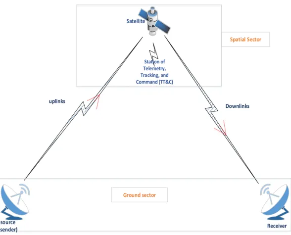
General Overview of Satellite Communications 10 Station of Telemetry, Tracking, and Command (TT&C) Satellite Downlinks uplinks Spatial Sector Ground sector source (sender) Receiver

Figure 1-1: A component of satellite communication system.

Ground Sector

The ground sector is made up of all earth stations, most often connected to users' terminals by a terrestrial network or directly in the case of small stations (VSAT: very small aperture terminal) and mobile stations. The stations are distinguished by their size, which varies according to the type of traffic (telephone, television, and data. A distinction is also made between fixed stations, transportable stations and mobile stations. Some stations are both transmitting and receiving stations. Others are receive-only (RCVO: receive only): this is the case, for example, of the receiving station of a satellite broadcasting system, or of a television or data distribution system [12],[13]. The cost of earth stations can be a determining factor in a communication network for which security, availability and reliability of equipment are prime requirements.

Space Sector

The space sector comprises the satellite and all the ground-based control means, in other words all the tracking, telemetry, and command (TT&C) stations, as well as the satellite control

(14)

center where all the operations related to station-keeping are decided and the vital functions of the satellite are verified [12].

1.2.2.1 Definition of the communications satellite

The satellite is naturally the essential part of a satellite communications system. At the beginning of the 1960s, when various possibilities of space telecommunications were being tested [1, 2], the satellite was a purely passive object, a large reflecting sphere moving in the sky whose only function was to reflect the received energy, but the poor results obtained led to the abandonment of such a system.

The satellite is now of the active type: it behaves like a real radio relay in the sky. It receives emissions from the earth (uplink) and retransmits them back to earth (downlink) after frequency translation and amplification. There are many kinds of satellites [14],[15]:

 Astronomical satellites: they observe space as they are placed above the atmosphere, they can see the stars and black holes better because they are not hindered by the layer of air and pollution.

 Navigation satellites: they are used to track the position of ships and marine currents.

 Meteorological satellites: they are used to take pictures of the earth, the pictures allow to forecast the weather. They are either geostationary or in constant rotation around the earth.

 Telecommunication satellites: telecommunication satellites are used for telephone communications, television pictures and radio.

 The military satellites: there are two types of military satellites: telecommunication and surveillance (terrestrial and maritime reconnaissance) as soon as a satellite has accomplished its mission, there are two ways to get rid of it:

(15)

12 2. It is allowed to fall back to earth: scientists calculate that it will fall back to an uninhabited area (often in the middle of the ocean). If it is small, when it reaches the atmosphere it disintegrates due to friction with the atmosphere.

1.2.2.2 Construction of a telecommunications satellite

The satellite is made up of a payload and a platform: The platform comprises all the subsystems that enable the payload to operate. We find:

 Power supply: all satellites need power to operate. The sun provides the energy needed for most satellites in orbit. This power supply system uses solar panels to convert light into electrical energy, batteries to store it, and a distribution system that transmits the electrical energy to each instrument.

 The control system: This system controls all of the satellite's functions. It is the satellite's brain. The heart of this system is called the Flight Computer. There's also an input/output processor that redirects all the control data that goes in and out of the Flight Computer.

 Altitude and orbit control and propulsion equipment: this system allows the satellite to remain stable and always be oriented in the right direction. The satellite has sensors that allow it to know its orientation. In addition, the satellite also needs to be able to move to correct its position, which is why it has a propulsion mechanism. The performance of the altitude control system depends on the use of the satellite. A satellite used to make scientific observations needs a more accurate control system than a communications satellite.

 TT&C tracking, telemetry and remote control equipment: this equipment consists of a transmitter system, a receiver system and various antennas to relay information between the Earth and the satellite. The ground control base uses this equipment to transmit new instructions to the satellite computer. This system also allows the transmission of images or other forms of recorded data to engineers on Earth.

 Thermal control: the system protects all satellite equipment from damage due to the space environment. In orbit, a satellite is exposed to sudden changes in

(16)

temperature (from -120° when the satellite is in darkness, to 180° when the satellite is exposed to the sun). Temperature control uses a heat distribution unit and a thermal blanket system to protect the satellite's electronic equipment from these sudden temperature changes.

The payload of a satellite represents all the equipment enabling the satellite to perform the function for which it is intended. For a communications satellite, the payload may represent the antennas reflecting the TV signal or the telephone signal. For an observation satellite, the payload consists of digital cameras and image sensors to take pictures of the Earth's surface. This payload consists of a set of channels, each channel being equipped with a transmit amplifier operating in a particular sub-band of the total band allocated to the satellite. This arrangement makes it possible to offer, in each channel, a power level commensurate with the state of technological development of the on-board microwave amplifiers, whereas the implementation of a single amplifier for the entire band would lead to a dissemination of the power of this amplifier.

Figure 1-2: Satellite structure [12].

1.2.2.3 Service provided by satellite

There is a strong demand for personal and mobile services. Recently, the notion of multicast service, i.e. from one source to a specific group of users, has emerged. This definition is to be contrasted with broadcast, which floods an entire region with users without any distinction other than geographical. In any case, this desire to share information makes relays

(17)

14 The distribution map between satellite networks and terrestrial networks is therefore changing radically in a synthetic way, the advantages of satellites are as follows:

 The covering of large geographical areas.

 The possibility to have multiple accesses and distinctions for the same Communication.

 The possibility of quick deployment of services.

 Adaptation to regions without telecommunications infrastructure.

 Observing the land, climate, plants and oceans.

 Transmit the waves: radio, television, telephone, and internet.

The waves they send out travel at 300,000 kilometers per second.

1.3 Orbits Tracked by Satellites

Satellites use the gravitational force of our planet in order to keep themselves at a certain position and distance from the earth. It is thus possible to define at any time what the characteristics of the satellite are in order to establish transmissions. We will see in this section what types of orbits are used and how they set certain limits or constraints in transmissions or equipment [16],[17].

 The orbit is the ideal trajectory that a satellite follows in the absence of disturbances.

 Orbits are usually classified according to their average altitudes and their synchronization with the earth or the sun.

Three different types of orbits can be distinguished: geostationary or geosynchronous orbit, medium-altitude or medium Earth orbit and low-altitude or low Earth orbit, each with different characteristics from the others [17].

We can also classify these orbits according to their shapes; in this case we distinguish two types: circular orbits and elliptical orbits.

(18)

Circular orbits

There are an infinite number of circular orbits, each corresponding to an inclination with respect to the orbital plane, but two kinds can be distinguished: the polar circular orbit and the inclined circular orbits [16].

1.3.1.1 Polar circular orbit:

The polar orbit is a circular orbit that passes over both poles of the earth. The main disadvantage for satellites in this type of trajectory is the slowness of their coverage, but this low speed still allows the satellite to cover a large part of the surface of the globe, or even the entire earth, given the rotation of the earth on itself. One example is the French observation satellite "Spot", located at an altitude of 800 km, which provides coverage of the entire surface of the globe in 21 days [18],[19].

1.3.1.2 Inclined circular orbit:

Inclined circular orbits also describe a circle around the earth, but each path is inclined at an angle to the equatorial plane. However, this inclination has a major disadvantage: since the highest latitude served by satellites with inclined orbits corresponds to the angular deviation from the equatorial plane, these satellites cannot cover the entire surface of the globe, but this orbit has an advantage: depending on the altitude of the satellite, it is possible to target areas of the globe, i.e. to serve parts of interest from the economic, military or other applications [16].

For example, the French project "Globalstar" plans to launch 48 satellites into a circular orbit inclined at 50° to the equator to provide mobile communications in most countries.

These two types of trajectories each have different characteristics, with different uses depending on the disadvantages and advantages. Nevertheless, they are used very little in comparison with the geostationary orbit, which currently has the most economic and practical advantages.

(19)

16

Polar Orbit Inclined circular Orbit

Geostationary Orbit

Figure 1-3: Circular orbits.

Elliptical orbit

As the name implies, a satellite placed in such an orbit describes an elliptical trajectory around the earth. The main characteristic of this type of orbit is the great variation in speed that the satellites undergo [17]. Indeed, the farther a satellite is from the earth, the lower its speed is because the speed "v" is inversely proportional to its altitude "h" according to the relation:

𝑣2 _{= 𝐺 ∗ 𝑚 ∗ (}2 ℎ−

1

𝑎) (1-1)

Where G is the gravitational constant, m is the mass of the satellite and has the half-major axis of the orbit.

Elliptical

o

rbit

(20)

However, because the altitude varies greatly during its period and the trajectory describes an ellipse, the position of the satellite for a ground-based observer is not fixed. Therefore, the tracking of each satellite requires the equipment of transmitting and receiving stations with mobile antennas, which is considered a disadvantage from a financial and qualitative point of view. Nevertheless, satellites in elliptical orbits have the advantage of being able to serve areas far from the equator, which is not necessarily the case for circular and geostationary orbits. This is not necessarily the case for circular and geostationary orbits, since with a high inclination, it is possible to fly over territories on the periphery of the hemispheres. The atmospheric layer being narrower, the quality of the signals is therefore a little better [12].

For example, in the "Molnya" system used by Russia, 3 satellites whose orbits are inclined at 63° to the equatorial plane, cover Siberia completely because their slow parts correspond to two thirds of their period and they are then located vertically over the Siberian territory [12],[13].

Elliptical orbits have advantages, such as coverage of areas far from the equator, but also disadvantages such as the qualitative and financial aspects of mobile equipment on earth. For circular orbits, however, these disadvantages are almost non-existent.

1.4 Satellite constellations

A satellite constellation can be defined as several similar satellites of the same type having the same function and designed to be similar, complementary and orbiting for a common purpose under shared control [20],[21].

There are three types of constellation according to their orbital altitudes:

Low Earth Orbit Constellation

Satellites in low orbit describe elliptical or (more often) circular orbits within 2,000 kilometers of the earth. The orbital period at these altitudes is between 90 minutes and two hours. As for the radius of the coverage area, it is between 3000 and 4000 km [17].

A LEO satellite can remain visible for up to 20 minutes for an observer on earth.

A global transmission system using this type of orbit required a large number of satellites in a number of different orbital planes. When a satellite in charge of a given user is no longer

(21)

18 visible to that user (it passes below the visible horizon), the satellite must be able to transfer the services for which it was responsible to another satellite in orbit identical or adjacent: this is the management of the hand-over [12],[17].

LEO constellations in any case offer particularly low propagation delays, of the order of around 20 ms, which allow them to provide services of the same type as those of terrestrial wired fiber optic networks.

Medium Earth Orbit constellations

ICO or MEO (Intermediate Circular Orbits, Medium earth orbits) satellites describe circular orbits at an altitude of about 10,000 kilometers. The orbital period is about 6 hours and an earth observer can have a visibility of a satellite of a few hours [12],[22].

A global transmission system using this type of orbit requires a smaller number of satellites compared to the LEO constellations. Only 2 to 3 orbital planes are needed to achieve global coverage.

An MEO-type constellation works very similarly to LEO systems; however, by structure, there is obviously less need for a hand-over system.

The propagation delay is greater than in LEO constellations, but still much less than in GEO systems.

GEO Constellation

The most commonly used satellites for telecommunication purposes are geostationary satellites. The altitude of these equatorial satellites, such that their orbit period is synchronous with the earth, i.e. one rotation in 23h 56mn 4s, will be approximately 36,000km. Three satellites placed at 120° on the geostationary orbit allow to "seeing" almost the whole earth, except for a small polar zone located at the extremes (Fig. I.5). The propagation delay is greater than in the LEO and MEO constellations [12],[21].

(22)

Figure 1-5: GEO constellation.

1.5 Geometry between earth and satellite

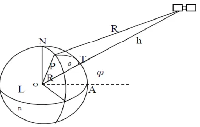
Each satellite is defined by its latitude and longitude relative to a reference point p [12].

Figure 1-6: Geometry between earth and satellite.

Where: φ is a satellite latitude; λ: satellite longitude; l: latitude of a point of satellite longitude; θ: longitude of P; L= θ -λ: difference in longitude of satellite and point P; h: satellite altitude; RT=6378Km: earth radius; r=RT+h: distance between the centre of the earth and the satellite; 𝑅 = √𝑅𝑇2+ 𝑟2− 2𝑅_𝑇𝑟𝑐𝑜𝑠∅: Distance between the satellite and point P With 𝑐𝑜𝑠𝜑 = 𝑐𝑜𝑠𝐿. 𝑐𝑜𝑠𝜃. 𝑐𝑜𝑠𝑙 + 𝑠𝑖𝑛𝜃. 𝑠𝑖𝑛𝑙

Two angles are used to locate the satellite from a point P on the earth's surface, usually the elevation angle and the azimuth [23].

(23)

20  The elevation angle El is the angle between the horizon at the point in question

and the satellite, measured in the plane containing the point in question, the satellite and the center of the earth.

 The azimuth angle A is the angle, measured in the horizontal plane at point P, between the direction of true north and the intersection of the plane containing the satellite and the center of the earth.

Figure 1-7: Nadir angle and elevation angle.

 Another useful angle is the nadir angle S. This is the angle at the satellite between the direction of the centre of the earth and the direction of the reference point P.

1.6 Basics of space mechanics

We consider the evolution of a mobile assimilated to a material point in the vicinity of a celestial body. It is assumed that [23]:

 The only forces taken into account are the Newtonian forces of attraction.

 The celestial body is assumed to be spherically symmetrical and of constant mass distribution.

Under these conditions, the study of the motion of the mobile can be assimilated as a first approximation to a 2-body problem: a particle of mass m attracted by a particle of mass M.

(24)

Kepler's laws

1.6.1.1 First Law or Law of Orbits

In the heliocentric frame of reference, the orbit of each planet is an ellipse with one of its foci occupied by the sun [16],[17].

Figure 1-8: The ellipse.

In fact, the first law states that all orbits have the shape of an ellipse. This law does not prohibit circular orbits, in fact the latter are considered as ellipses whose two foci are confused.

1.6.1.2 Second Law or Area Law

The motion of each planet is such that the line segment connecting the sun and the planet sweeps equal areas for equal lengths of time [16].

Figure 1-9: Law of areas.

1.6.1.3 Third Law or Law of Periods

For all the planets, the ratio between the cube of the trajectory's half-major axis (a) and the square of the period (T) is the same [12],[16].

(25)

22

𝑇2

𝑎3

= 𝑐𝑡𝑒

(1-2)

This means that the time it will take the satellite to complete one orbit (period) can be calculated from half the dimension of the half-major axis.

The law indicates that the satellite will have a slower speed at higher altitudes and conversely a faster speed at lower altitudes.

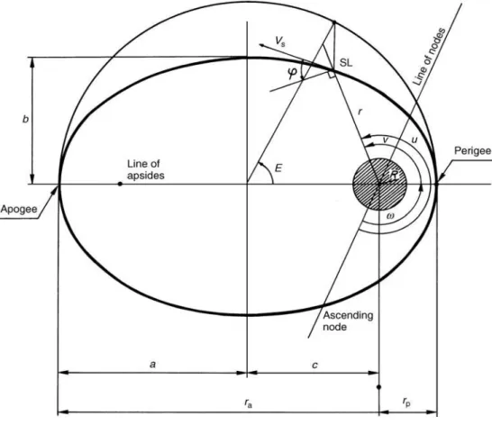
Orbital parameters

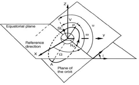
An elliptical trajectory is characterized by six orbital elements (corresponding to six degrees of freedom). Two define the shape of the ellipse: a and e which are respectively the semi-major axis and the eccentricity. Three orbital elements are used to orient the position of the ellipse in space: w, Ω, i, respectively the perigee argument, the right ascension of the ascending node and the inclination [12],[13].

(26)

1.6.2.1 Reference axis

The satellite's orbit crosses the plane of the equator at two points called the descending node ND at the northern hemisphere to southern hemisphere crossing point, and the ascending node NA at the northern hemisphere crossing point. The line (NA, ND) is the line of nodes [16],[24].

1.6.2.2 Parameters defining the position of the orbit plane

We know by Kepler's first law that motion is plane and that the trajectory has the shape of an ellipse [12].

Figure 1-11: Position of the orbit plane.

We can therefore define 2 angles allowing to position the plane of the orbit with respect to an initial equatorial reference frame :

I= the inclination with respect to the equator.

Ω= the right ascension of the ascending node i.e. the angle between the X axis and the line of intersection of the plane of the orbit with the equator (longitude).

The node line (NA, ND) bisects the equatorial plane and the orbit plane.

 The angle I formed by the half-plane of the orbit containing the satellite's trajectory from NA to ND and the half-plane of the equator containing the

(27)

24 from 0° to 180°. The orbit is said to be direct when i is less than 90° and retrograde when i is greater than 90°.

 The angle Ω which, in the plane of the equator, forms the node line and the direction of the vernal point, defines the orientation of the node line. It is the straight ascent of the ascending node which is measured from 0° to 360°, from the vernal point to the ascending node, in the direction of rotation of the earth or direct direction.

1.6.2.3 Orbital shape and position

In the plane of the orbit, the ellipse itself is characterized by two parameters:

a: the semi-major axis, b: the semi-small axis.

We very often replace b by the eccentricity e, knowing that

𝑏2 _{= 𝑎}2_{(1 − 𝑒}2₎ _(1-3)

Then defines an origin on the ellipse; conventionally, we are used to locate it at the perigee (the point closest to the earth) of the orbit.

The position of the major axis in the plane of the orbit is defined by the angle ω, formed by the line joining the center of the earth at perigee on the one hand and the line of the nodes on the other. It is the argument of the perigee ω, which is measured from 0° to 360°, from the ascending node to the perigee in the direction of the satellite's revolution.

1.6.2.4 Position of the satellite in orbit

Now we need to know exactly where the satellite is positioned on the ellipse [16].

The angle determining the position of the satellite relative to the perigee can be expressed in different ways:

V= the varying anomaly actually corresponds to a polar coordinate.

E=the eccentric anomaly by projecting the satellite on the main circle of the ellipse

(28)

This fictitious angle M makes it possible to simply define the Keplerian motion as a function of time by:

𝑀 = 𝑀₀+ 𝑛(𝑡 − 𝑡₀) (1-4)

Where n is the mean motion equal to:

𝑛 = √

_𝑎𝜇3 (1-5)

In addition, constant due to Kepler's third law. We thus obtained 6 orbital parameters: 𝑎, 𝑒, 𝑖, 𝜔, Ω, 𝑉 𝑜𝑟 𝐸 𝑜𝑟 𝑀.

The main advantage of the Keplerian parameters is that, if the disturbances are not taken into account, the first five are constant over time while the sixth (V, E or M) varies linearly with time.

Orbital perturbations

There are a number of physical contributions that influence the trajectory of a body in Earth orbit. These are called perturbations and if it is not always possible to take them into account analytically in the calculation of the orbit, it is necessary to take them into account, for example, to make periodic corrections to the trajectory.

There are various numerical methods [13] to evaluate these disturbances

1.6.3.1 Perturbation of the third body

The presence of the sun and moon causes variations in all orbital elements, but the secular (long-term linear) effects are mainly on the right ascension ω and the perigee argument ω [1],[16].

For satellites with circular orbits and a higher attitude than a geostationary one, this disturbance predominates.

(29)

26

1.6.3.2 Disturbance due to the non-spherical earth

For satellites whose orbit is less than or equal to a geostationary orbit, it is the effect of the flattening of the earth at the poles that dominates, causing variations on the right ascension and the perigee argument [12].

1.6.3.3 Disturbances due to atmospheric friction

This is the main force of non-gravitational origin that affects satellites in Low Earth Orbit (LEO). This friction causes them to lose kinetic energy and therefore altitude. As a result they can end up re-entering the atmosphere if the trajectory is not compensated [5].

1.6.3.4 Solar radiation perturbations

At altitudes above 800 Km, another disturbance takes precedence over atmospheric friction: the pressure due to solar radiation which causes an acceleration, applied in the direction of the sun, equal to [5],[13]:

𝑎 = −4.5. 10−8_𝐴/𝑚 _(1-6)

Where A is the surface exposed to the sun and m the mass of the satellite.

1.6.3.5 Intrinsic perturbations

There is a range of disturbances that depend directly on the construction of the satellite. Among them are the following [5],[12]:

 Uncertainties about the center of Les gravity.

 Uncertainties about propulsion.

 The vibration modes of the structure.

These intrinsic disturbances mainly concern the attitude (the angular position of the satellite and its variation with respect to time) of the satellite but can also indirectly influence the orbital trajectory.

(30)

Maintenance and survival in orbit

The earth contains strong magnetic fields, which affect its surroundings. Specifically, some areas beyond the earth's surface have radiation levels high enough to damage electronic components that pass through them [12],[25].

At high altitudes, the Earth's magnetic field is strongly distorted by the pressure of the solar wind, and at low altitude and (LEO), it is approximately that of a dipole tilted about 11.5 degrees from the Earth's rotation axis.

One of the most important effects of the Earth's magnetic field, in terms of engineering is due to Van Allen's belts, named after the American physicist who discovered them in 1958. They are two toric zones, where the electron concentration and of protons is very important because they have been trapped by the magnetic field [19]. The first belt is between 600 and 90000 Km of altitude for a latitude between +40° and -40°; the second is located at an altitude of about four times the Earth's radius and largely overlaps the first [12].

There are four main regions where satellites are put into orbit:

 The LEO (Low Earth Orbit) zone, between the end of the atmosphere and the first Van Allen belt, from 400Km to 1500 Km of altitude.

 The MEO zone (Medium Earth Orbit), between the two Van Allen belts, from 5000 Km to 13 000Km of altitude.

 The HEO (High Earth Orbit) zone, whose apogee is beyond the Van Allen belts, but which, within the framework of elliptical orbits, encompasses one or more of the previous zones.

 The GEO (Geostationary Earth Orbit) zone, which could be seen as a special case of HEO, for geostationary satellites, at an altitude of Seventy-five thousand miles.

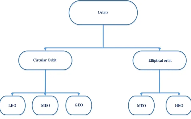
It is not interesting to place a satellite with an elliptical orbit in the LEO area, given the small margin that one has (the main half-axis and the minor half-axis are both between 7 000 Km and 8 000 Km). There is still the possibility of placing them in orbit, or passing them through the Van Allen belts, which reduces the lifetime of the electronic components. In summary, the classification in figure (I-12) can be considered [12].

(31)

28

Orbits

Circular Orbit Elliptical orbit

MEO GEO MEO HEO

LEO

Figure 1-12: Classification of the different types of exploitable orbits.

1.7 Conclusion

In this chapter, we provided a comprehensive description of the communications by satellite. We also talked about the types of orbits in terms of form, which led us to address mentioning the types of satellite and the characteristics of each satellite, the appropriate orbit for each satellite and the minimum number of satellites to cover the globe also the distance of the satellite and the globe. In addition, we discussed geometry between satellite and Earth and some of the basics of space mechanics. Finally, we described how to maintain the satellite in orbit, and what is its expected lifetime.

In the next chapter, we will talk in detail about optical communications, especially lasers, their origin and stages of development, up to the application of their use in the satellite.

(32)

Optical Telecommunications and the Effect of Atmosphere

CHAPTER II:

Optical Telecommunications and the Effect of

Atmosphere

(33)

30

2 Optical telecommunications and the effect of

atmosphere

2.1 History of optical telecommunications

In this chapter, we will try to make a historical overview of the techniques that humans can set up to establish connections using optical signals. While focusing on some important technical advances as they reflect the principle of Atmospheric Optical Link (AOL).

The idea of using an optical signal to communicate is not new. The light spreads naturally and the eyes are already a powerful detector for this type of signal. In Antiquity, ancient Greeks used mirrors directed to target ships, or dangled their shields to communicate in battle. The succession of sent signals constituted a Morse coded message.

The main limitations are then the range and the flow of information transmitted reduced. Claude Chappe made a first progress in 1794 in terms of flow [26]. By observing with binoculars the position of the arms of a pantograph at the top of a tower, the operator is sent back to a number corresponding to an agreed-upon message (birth of telegraphy). However, the real precursory contribution of the AOL is the proposal of Maurat, taken by Mangin. It consists in improving the directivity, therefore the range, of the optical signal emitted by a set of mirrors and simple lenses collimating the beam (Figure 2-1). Thus, in 1873, with optics 30 cm in diameter, this device allowed to work on ranges of 36 km at a rate of the order of 200 words per hour.

(34)

Optical Telecommunications and the Effect of Atmosphere Telescopic device Reception Window Oil Lamp Mirror

diaphragm control lever

lens

Figure 2-1 :Optical telegraph of Mangin [27].

With the invention of the photophone in 1880 (see figure 1.2), Graham Bell demonstrates the effectiveness of the use of an optical signal (here solar radiation) to transmit information, the voice [27], using the intensity modulation. The distance it establishes is 200m [28].The variability of the light source (the sun) and the short propagation distance limited by the low sensitivity of the detection system will be the reason for its invention.

Figure 2-2: Schematic representation of Graham Bell's photo phone [27]. Under the influence of speech, the mirror deforms and modulates the intensity of the light coming from the sun as it reaches the receiver. The resistance of the selenium receiver varies according to

(35)

32 The telecoms initially abandoned the optics for the benefit of electronics. Indeed, the advent of electronics allows a modulation and demodulation of the signal much faster, telecommunications know their true revolution. The first wired networks date from the 19th century. They guide a message electrically and solve at once the problem of range and flow. First copper cables were thrown in 1850 into the Atlantic Ocean to allow telegraphic communications between Europe and America. This date corresponds to the control of the insulation of cables under water [29].

To overcome the wired network, it was again necessary to look into the free space propagation of an electromagnetic wave. The first breakthrough in this direction was achieved in the range of radio waves, the propagation of which is not altered by atmospheric turbulence. It will be seen later that this is not the case in the optical range.

Thus, in 1896, Marconi transmits and captures signals over a distance of 250m, having synthesized the inventions of Alexander Popov's antenna, the Branly electromagnetic wave detector and the principles of the established radio program by Tesla. Three years later, the latter made the first radio communication program between France and England [29].

The scientific community has been trying, since the 1960s and the invention of the laser, to set up free space communications using an optical signal to establish a direct line of sight link. The first applications are developed for links to satellites [30],[31]. Unfortunately, the limited lifetime of lasers, their size and insufficient light output cause the rapid decline in interest in this technology.

In the 1980s, the appearance of semiconductor lasers with long life span, low footprint and high efficiency, contributes to the emergence of laser communication programs from Europe and the United States. United States [32],[33]. Lasers, being high-power directive sources, make it possible to work with high signal-to-noise ratios (SNRs) when they are associated with modern detectors, which was lacking in Bell's photophone.

Again, the challenge is to achieve the same quality of telecommunication with free-space signal propagation. This is the purpose of AOLs. Under certain conditions, favorable in terms of atmospheric turbulence encountered, namely telecommunications in space or from space to the ground, AOLs have already appeared:

(36)

 In 2001, the first unidirectional satellite-satellite optical link (SILEX project) which enabled the transfer of data from the ARTEMIS satellite to SPOT 4 [22],

 In 2002, the first two-way ground-to-satellite optical link between the Optical Ground Station built at the Mount Teide Observatory (Canary Islands) and the ARTEMIS satellite (SILEX project) [34],

 In 2006, the first two-way satellite-to-satellite optical link between the ARTEMIS and OICETS satellites (Japan) [35],[36]

 In 2006, the first optical link between a satellite (ARTEMIS) and an aircraft (Mystery 20) of 50 Mbits / s (LOLA project) [37],

 In 2007, the first bidirectional ground-to-satellite optical link between the KIRARI satellite and a mobile telescope of 0.4 m diameter of the DLR [36].

However, outside the experimental setting, the transfer of data on the ground is still done by radio frequencies, with a much lower flow rate. For endo-atmospheric propagation, the use of radiofrequencies is all the more justified by the main limitation encountered by AOLs: propagation through the atmosphere.

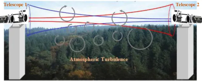
2.2 Principle and characteristics of atmospheric optical links

Atmospheric optical links (AOLs) rely on the propagation of light in free space to transmit information between two points. These links are usually to-point, but there are also point-to-multipoint links. The different areas of AOL applications (air-to-air links, satellite-underwater, air-submarine, air-satellite, satellite-satellite, etc.) have a major impact on their characteristics and their locations. It is, therefore, difficult to have a general discourse encompassing all AOL systems. We only consider AOLs as part of an air-to-satellite line of sighting line. Figure 2-3 shows schematically an atmospheric optical link in the case of a point-to-point application between two urban sites. AOLs make it possible to overcome the disadvantages of a fiber-optic type connection, which is often long and expensive to set up. In addition, the absence of the license requirement, interference immunity as well as natural link security (directional beam) that can operate in full-duplex (Telecommunication system where the signal is transmitted in both directions simultaneously) and the possibility of reaching high transmission rates are additional advantages over conventional wireless communications.

(37)

34

Telescope 2 Telescope 1

Figure 2-3: A modern optical telegraph

A modern optical telegraph, or AOL, consists of two distant telescopes facing each other, each with emission and laser detection. Each telescope simultaneously transmits and detects the stream emitted by the other, thus creating a bidirectional optical link in direct line of sight (Figure 2-3).

For a civilian use, this device must be reproduced identically to renew the range of the signal and thus grid a given territory. The telescopes should be placed at least 30 meters above the ground to avoid physical obstacles. This also has the advantage of avoiding the most turbulent air layer at ground level (see §2.3.1 The physical phenomenon of turbulence) [38].

Modulation of AOLs endo-atmospheric

Free space propagation can benefit from the same modulation and demodulation technologies as those developed for guided optics. Modulation techniques include On-Off Keying (OOK), which is simply based on modulating the amplitude of the source to encode binary information. However, there are also more subtle strategies, such as Pulse Position Modulation (PPM) [39], which requires less average energy than the OOK modulation for the same error rate on reception. On the other hand, PPM requires greater bandwidth and more difficult reception timing [40]. We limit ourselves in the following of the manuscript to the case of the modulation OOK.

(38)

Benefits of AOLs endo-atmospheric

Free space telecommunications are nowadays very common use in the terrestrial range. However, the optical range has much shorter wavelengths to modulate the signal much faster, and thus increase the rate. Thus, optical telecommunications allow considering rates well above the 10Gbit/s [41]. Moreover, with respect to a strongly diverging radio emission due to the diffraction (high wavelength), the laser emission is very directive. This gives him several advantages:

 The communication is more secure because difficult to intercept;

 There is no bandwidth to share because the environment is not drowned out signal;

 It is possible to reduce the transmission power.

It is possible to combine all these qualities with guided optics. However, the propagation in free space differs from a fiber network by the following aspects:

 Implementation of the immediate network;

 Portability;

 Lower installation cost;

 Mobile target tracking.

Thus, there are applications for which it is not possible to extend a cable and which may require a much higher rate than that offered by a microwave link. One can imagine for example the rapid implementation of an AOL on a disaster area by an earthquake that broke the existing fiber network. The AOL would provide for the speed and quality of on-site intervention. On the other hand, the saturation of an urban network following the organization of an exceptional event, which does not justify the permanent increase of the capacity of the network [42].

The AOLs can thus provide a high-speed telecom connection at a given moment, without investing the necessary sums for the installation of a new fiber network.

(39)

36

The limitations in atmospheric optical links

Optical communication has grown rapidly because it provides a stable propagation medium that limits the loss of flux during propagation. In the case of a AOL, the propagation medium is the ambient atmosphere that has two main limiting factors:

 Attenuation of the signal;

 Degradation of the optical quality of the laser beam.

Concerning attenuation, a drop in the received signal necessarily induces a decrease in the range of the system. In the visible range, the attenuation by the atmosphere is very dependent on the climatic conditions (fog, rain ...) [43],[44]. Apart from the choice of a transmission wavelength at a minimum of attenuation by the atmosphere, the increase of the flux is the only possible solution to bring [45].

The degradation of the quality of the laser beam during propagation has, for its part, other origins. The atmosphere being a turbulent medium, the inhomogeneity of the medium can deflect or even burst the beam, so that it is no longer detected by the target. As the impact of atmospheric turbulence increases with the volume of turbulence traversed, the system is limited in scope. However, one can imagine solutions such as the pre-compensation of the beam at the emission to mitigate the effects of the turbulence [46]. For example, in the case of deflection from the beam by the turbulence, the beam can be emitted in another direction of propagation so that the turbulence brings it back to the target. The study of signal propagation allows us to develop precompensation strategies to overcome the limitations introduced by turbulence [47].

2.3 Atmospheric turbulence

The physical phenomenon of turbulence

Theorists such as Poiseuille, Reynolds later followed by Taylor and Von Karman, gave the first definition of turbulence as “an irregular movement that appears in fluids when they encounter solid obstacles”. At the beginning of the 19th century, Claude Navier wrote the basic equations governing the temporal evolution of the flow of a fluid in turbulence [48].

(40)

Figure 2-4:An overview of the principle of energy cascade in a fluid in turbulent flow where the transfer is from large to small scale [48].

The Earth's atmosphere is made up of a gas mixture in perpetual evolution. On the one hand, it is heated by solar radiation, and on the other hand, it undergoes radiative interactions with the ground. The temperature in the atmosphere is therefore highly inhomogeneous. This results in the formation of air masses of different densities. Under the effect of gravitation, these air masses are set in motion and interact constantly. A turbulent flow is created at their interface: it is the formation of turbulent layers. These layers are characterized by local variations in temperature, pressure, and humidity, which cause local variations in the refractive index of the air. These fluctuations cause a disturbance of the propagation of electromagnetic waves [49].

Theory of energy cascades

Kolmogorov [48] proposed a statistical description of the phenomenon of atmospheric turbulence, based on scale laws [50]. A turbulent flow leads to the formation of large vortices, the kinetic energy of which is transmitted to smaller and smaller vortices, in the form of a cascade of energy, until dissipation by viscous friction.

(41)

38

Figure 2-5: Schema of the energy cascade process and the division of turbulence cells in the atmosphere.

 Inertial domain: Spatial scales for which the turbulence is said to be fully developed and for which the Kolmogorov model applies define the inertial domain. It is bounded on the one hand by the size of the largest vortices, of the order of a few tens of meters, and on the other by the size of the smallest vortices, of the order of a few millimeters.

 The external scale: The external scale L0 is the magnitude characterizing the spatial

dimension of the largest eddies. Its size influences the amplitude at low spatial frequencies of phase disturbances due to turbulence. For future large telescopes, whose diameter will be several tens of meters, the influence of the external scale becomes significant, and one needs to access to its measurement. Several techniques nowadays make it possible to estimate L0.

The Generalized Seeing Monitor (GSM) uses fluctuations in the arrival angle of the wavefront [51],[52],[53]. The external scale can also be deduced from interferometric data[54], or data from adaptive optics [55]. Finally, the Monitor of Outer Scale Profile (MOSP) provides access to external scale profiles as a function of altitude [53],[54], from the correlations of wavefront arrival angle fluctuations measured on lunar edge images. The typical value of the external scale is generally of the order of a few tens of meters [56].

 The internal scale: The internal scale 10 corresponds to the spatial dimension of dissipation of the kinetic energy by viscosity. Studies offer techniques to access its value. Some use angle of arrival fluctuations [57],[58], others intensity fluctuations [59],[60]. It is also possible to estimate 10 from the scanning effect of a laser beam [57],[61]. Finally, there

(42)

are hybrid techniques that use both phase and intensity fluctuations [62]. The typical value of the internal scale is generally of the order of a few millimeters.

The refractive index of air

2.3.3.1 Fluctuations in the refractive index

Consider the difference between the value n (r) at a point r and the value n (r + ρ) at a point distant from a distance ρ. The vectors r and ρ respectively represent a position and a separation distance in a three-dimensional space.

For an established turbulent regime (temporally and spatially stationary), in the inertial domain, the variance of the difference of the refractive index at two points of space, or function of structure, is given by [63],[64]:

𝐷_𝑛(𝜌) = 〈|𝑛(𝑟) − 𝑛(𝑟 + 𝜌)|2_{〉 = 𝐶}

𝑛 2. 𝜌2⁄3 (2-1)

Where the brackets ⟨⟩ represent the overall mean. Dn(ρ) is called the structure function of the refractive index and 𝐶_𝑛2_{is the structure constant of the refractive index. 𝐶}

𝑛2 is expressed in

m-2/3 and ρ = | ρ | is expressed in m.

Equation 2.1 is actually only a valid approximation as long as ρ is smaller than the external scale of turbulence. However, for the great distances ρ, the values n (r) and n (r + ρ) will become complementarily independent. According to equation 2-1, the fluctuations of the refractive index are then at infinity, which has no physical meaning. Dn (ρ) is only valid for l0

< ρ <L0.

2.3.3.2 Spectral density of index fluctuations

Obukhov and Yaglom [63],[64] have shown that the power spectra of temperature and humidity fluctuations follow the law in f-11/3. A power law in f-11/3 also describes the fluctuations of the air index, directly related to these two parameters.

Tatarski gives the expression of the spectrum of fluctuations of index 𝑊_𝑛(𝑓⃗) valid between l0 and L0 [65]: