Hypothesis Test of the Photon Count Distribution for Dust
Discrimination in Dynamic Light Scattering
David Bossert,
†Federica Crippa,
†Alke Petri-Fink,
†,‡and Sandor Balog
*
,††Adolphe Merkle Institute, University of Fribourg, Chemin des Verdiers 4, 1700 Fribourg, Switzerland ‡Chemistry Department, University of Fribourg, Chemin du Musée 9, 1700 Fribourg, Switzerland
*
S Supporting InformationABSTRACT: Users of dynamic light scattering (DLS) are challenged when a sample of nanoparticles (NPs) contains dust. This is a frequently inevitable scenario and a major problem that critically affects the reproducibility and accuracy of DLS measurements. Current methods approach this problem via photon correlation spectroscopy, but remedy exists only for a few special cases. We introduce here a general criterion and a clearly defined measure to discriminate between NPs and dust particles. The experimental results show that, in contrast to photon correlation spectroscopy, hypothesis testing and the statistical moment analysis of the photon count distribution provides an accurate and precise way to character-ize NPs and Brownian dynamics in the presence of dust. To demonstrate, analyses of silica, iron oxide, and gold NPs of low polydispersity are presented.
T
he interest in nanoparticles (NPs) and colloidal phenomena stretches well beyond the classical realm of soft matter physics and physical chemistry,1 and by now, interdisciplinary topics, such as nanomedicine and nano-toxicology, have become key research areas. Their fundamental focus is on understanding and either exploiting or suppressing harmful interactions at the nano−bio interface.2−6 Dynamic light scattering (DLS) is one of the techniques found in any laboratory interested in measuring the size of NPs,7−10and yet, the nuances of the theory, the experimental procedure, and data analysis are frequently loosely interpreted. This is despite the efforts of emphasizing the importance of respecting the fundamental concepts again and again11−13 and proposing standardized procedures.14−17 Whether this is partially responsible for questionable reproducibility and for the setback in translating NPs into clinical applications18,19 is under debate.20,21Nonetheless, the gravity of this issue is illustrated well by the fact that national testing and metrology laboratories were unable to provide consistent DLS results on standard reference NPs dedicated to “evaluate and qualify methodology and/or instrument performance related to the physical/dimensional characterization of nanoscale particles used in preclinical biomedical research” issued by NIST (National Institute of Standards and Technology).22−24Although current DLS apparatus have high-quality parts and the underlying theory itself grants accurate and precise results,25−27 the quality of the experimental results, that is, the accuracy and precision of determining particle size, is dictated by the purity of the samples and by the capacity of the
algorithms regarding information collection, processing, and analysis to work with, in particular, dusty samples. In light scattering, dust is a generic term that refers to any foreign matter and impurities found in the sample, such as large particles, aggregates/agglomerates, traces, and remnants of the synthesis. The importance of sample purification, such as filtering, distillation, or centrifugation, cannot be stressed enough. Yet, there are situations where purification is neither applicable nor provides any desirable outcome.28 While the “number-averaged” presence of dust is usually negligible, e.g., they seldom appear on TEM micrographs, their unwanted “intensity-weighted” contribution to the scattering intensity in the form of unpredictable and anomalous fluctuations is significant enough to severely bias the results of the analysis. Despite the fact that DLS is a mature technique, this is still a major problem that critically limits the reproducibility and accuracy of the measurements, especially at lower scattering angles, because it artificially increases the apparent size and broadens the apparent size distribution. The simplest attempt in minimizing these deleterious outcomes is observing scattering in backward direction (near 180°), but this unfortunately limits the length-scale observed. Therefore, DLS analysis through photon correlation spectroscopy (PCS) and autocorrelation functions have been in the focus for a long time.29 To analyze the correlation function, the method of
http://doc.rero.ch
Published in "Analytical Chemistry 90(6): 3656–3660, 2018"
which should be cited to refer to this work.
cumulants30−34 and CONTIN35,36 are the most cited approaches, although many alternatives and improvements have been proposed.10,37−42 These include Bayesian analysis, maximum entropy, and neural network models.43−49All these approaches address the intensity auto correlation function, while it is well-known that the analysis of the correlation function is an ill-posed inverse problem, which becomes unreliable as soon as there is dust in the sample. In such cases, the correlation function displays multiple decays, and by inspecting solely the correlation function, one cannot discriminate between intensity fluctuations from, e.g., dust and those from larger but otherwise regular NPs. Also, given that each sample requires a different procedure, a different time range, the“...elimination of dust from a solution is considered by many to be a black art.”50 While certain special cases can be treated,51,52e.g., a nonzero baseline of the correlation function, it is impossible to give a universal recipe that guarantees a solution to the problem of corrupted correlation functions. To our knowledge, “dust-filter” algorithms of commercial instru-ments (Brookhaven, Wyatt, Anton Paar, Malvern) test either the average or the variance of thefluctuations of the scattering intensity obtained by short measurements and then identify and discard outliers by setting a threshold.53 We recognize three major shortcomings of this approach. First, when using this approach, it is inherently assumed that apart from outliers, most of the measurements are correct.53 Second, the threshold is more or less chosen arbitrarily for each sample and expected particle size. Third, it is not taken into account that the rate and the amplitude of the fluctuations is defined not only by the particle size but also by (a) the Brownian dynamics of the NPs, (b) the sample size collected, and (c) the integration time of counting the scattered photons, as shown elsewhere.54,55The consequence is the uncertain accuracy and reproducibility of the DLS analysis.
Here we present an alternative that circumvents these shortcomings. Based on the statistical properties of photon counting, we define a clear and rigorous criterion that allows differentiating between fluctuations originating from the coherent scattering of light from NPs and fluctuations originating from dust. Due to the Brownian motion of the NPs, the scattering intensityfluctuates randomly at an average rate that depends on the scattering angle and particle size:
Γ = Q D2 (1)
D is the translation diffusion coefficient of spherical NPs of radius r, πη = D k T r 6 1 B (2) where kBis the Boltzmann constant, T the temperature,η the viscosity of the solvent, Q the momentum transfer
= λπ
( )
θQ 4 n sin 2 , θ the scattering angle, λ the wavelength of the scattered waves, and n the refractive index of the suspension. Owing to the quantized nature of light, the detection of photons is never instantaneous and requires a finite time interval τ > 0. It can be shown that when 1 ≪ Γτ ≪ ⟨n(τ)⟩, where ⟨n(τ)⟩ is the mean photon number, and the integration timeτ is much larger than the coherence time of the intensity fluctuation due to coherent scattering, the photon counts are uncorrelated and the photon count distribution corresponding to the intensity fluctuations is symmetric and essentially follows a Gaussian distribution:54,55
π σ ≅ − −μ σ P n( ) 1 2 e (n ) /2 2 2 (3) μ = ⟨n(τ)⟩ and σ2=⟨n(τ)⟩2· (Γτ)−1, and⟨n(τ)⟩ is the mean of the photon count distribution. Accordingly, the relaxation rate can be determined directly from the variance and mean of the photon count distribution
τ
σ τ
Γ = ⟨n( ) 12⟩2
(4) Noncoherent outliers and drifts in thefluctuations will result in an asymmetry and an excess width, which distort the distribution of the photon counts. These critically affect the variance, the skewness, and the kurtosis of the experimental P(n). It is important to emphasize that particle polydispersity and multimodality, however, do not distort the shape of the photon count distribution. In such cases, P(n) is the convolution of the respective modes, and thus, remains Gaussian.54 This property lies at the heart of our approach, since a normality test performed on P(n) can decide with high certainty whether or not the intensity fluctuations are due to coherent scattering of light from NPs. Furthermore, if P(n) is accepted,eqs 1−4can be used for particle size analysis, without the necessity of constructing the correlation function.55 Therefore, the analysis of the photon count distribution of the scattered light enables (a) separating NPs from dust and (b) quantifying Brownian dynamics. If P(n) is Gaussian, the DLS data isfit for analysis, if not it is to be discarded. Testing univariate normality is a common procedure in statistics, and among the various tests,56the Shapiro−Wilk test57(SW) shows a very good performance.58 SW can be performed in R, Mathematica, Matlab, Octave, and online calculators are also available for free. SW is a goodness-of-fit test, with the null hypothesis that the particular set of data is drawn from a normal distribution. The test evaluates two mutually exclusive possibilities, accept or reject the particular set of data, by determining which possibility is supported better by the available data. SW determines the degree of closeness between the experimental data and the normal distribution via three steps:first, the data is standardized by subtracting its mean, and then by dividing the data by its standard deviation:
Δ = − ⟨ ⟩
⟨ ⟩ − ⟨ ⟩
n n n
n2 n2 (5)
In the second step, the standardized data is ordered. The standardized and ordered data (order statistics) now increases monotonically and has a zero mean and a unit variance. In the third step, the degree of closeness is quantified by the test statistic (0 ≤ W ≤ 1), which is essentially the measure of the Pearson correlation between the standardized and ordered data and the quantile function of the standard normal distribution. (The mean and variance of the standard normal distribution is zero and one, respectively.) The quantile function of the standard normal distribution, in other words, the inverse cumulative density function, is frequently referred to as the “Probit” function: f(x) = √2 Erf−1(2x− 1). From W, the p-value is calculated by taking into account the size of the data set. The p-value is by definition the probability of obtaining either W or larger than W given that the normality hypothesis is true. Therefore, the closer the value of p to zero, the stronger the evidence against accepting the data as normally distributed. As for any hypothesis test, the significance level (0 < α < 1)
dictates whether we shall accept or not the data characterized by a given p -value. The significance level is not derived from any observational data, independent of the nature of the hypothesis, and usually set prior to performing the test calculations. Usually,α = 0.05 or α = 0.01 are set, and hence the data is rejected if p <α.
To show the value of statistical inference in DLS experi-ments, we have synthesized silica NPs (Supporting Informa-tion, Materials).Figure 1shows two typical DLS results taken
from ten 10-s long measurements recorded atθ = 60° on the same sample. Although the sample was purified, the normality test concludes that only one of them is acceptable for analysis (Data A) and the other one is not (Data B). (In fact, from ten measurements, the normality test rejected three.) While the photon count distribution of Data B is asymmetric and strongly deviates from the normal distribution, Data A is symmetric and follows the normal distribution. For comparison, we also performed PCS analyses andfind that the field auto correlation functions of Data A and Data B are clearly different. Data B exhibits a prolonged second decay, whose impact is already clear in the cumulant analysis. The linear slope of the early decay of Data B is much smaller than that of Data A, and the apparent radii, estimated by the slopes of Ln g1are 106.1 nm (Data B) and 35.7 nm (Data A), respectively. There is a 3-fold difference between the two results, but the normality test rejects Data B, and hence, we discard this result. (We will show
later that the number given by the analysis of Data B is entirely inconsistent with the TEM result.)
To extend the use of statistical inference prior to the analysis of Brownian dynamics, we collected DLS data on a larger range (θ = 15°, 25°, 25°,.., 90°). Additionally, to make it clear that the statistical analysis of photon counts is effective even at low temporal resolution (PCS analysis requires submicrosecond temporal resolution), we set the integration time to 0.525 s and recorded photon counts during 10 s. After the normality test, the accepted photon counts were analyzed directly viaeqs 1−4
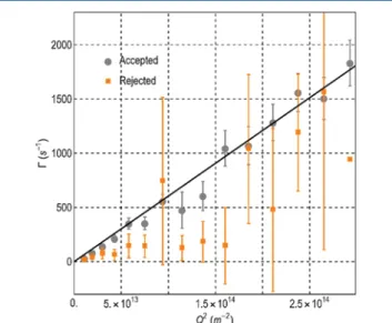
to determine the relaxation rate and hydrodynamic radius. Although the sample size was relatively low (s = 18), the expected relative accuracy is high (within 1%). The expected accuracy is calculated by following the steps explained previously.55 Only for comparison, the “apparent” relaxation rate of the rejected data were also computed. Figure 2shows
the Q2-dependence of the relaxation rate determined by the statistical analyses of the photon counts. The result shows that testing for normality effectively classifies the DLS data into two distinct groups. The set of data that was rejected by the hypothesis test is without a clear trend and display large uncertainty and, thus, indeed unsuitable for further analysis. In contrast, the set of data that passed the statistical test defined a straight line, as expected in the case of coherent light scattering from Brownian NPs in the dilute regime. The linear regression determines a radius of R = 36.5 nm, and the 95% confidence interval is 35.2−37.7 nm. To assess the extent of the quality of the results obtained via DLS and the normality test, the size of the SiO2NPs was also characterized by transmission electron microscopy (Figure 3, TEM, Supporting Information, Meth-ods). From TEM, fully independent of DLS, we determine a Z-average (⟨R6⟩/⟨R5⟩) of 35.9 nm. The agreement with our DLS analysis is excellent.
Figure 1. (a) Standardized photon counts of two 10-s long measurements recorded atθ = 60° (τ = 0.105, sample size s = 94) and (b) the distribution of the photon counts. The solid black line is the standard normal distribution. Data A is symmetric and appears to agree well with the normal distribution. Data B is asymmetric and strongly deviates from the normal distribution. (c) The order statistics together with the Probit function (solid black line). At α = 0.05 significance level the Shapiro-Wilk test rejects Data B (W = 0.87, p = 0), and accepts Data A (W = 0.99, p = 0.947). (d) The corresponding field autocorrelation functions. Data B exhibits a prolonged second decay, whose impact is clear, e.g., in the cumulant analysis (inset). The linear slope of the early decay of Data B is much smaller than that of Data A. Consequently, the apparent radii, estimated by the slopes of Ln g1are 38.7 nm (A) and 106.1 nm (B), respectively. The latter is
entirely inconsistent with the TEM result (Figure 3).
Figure 2. Q2-dependence of the relaxation rate determined by the
statistical analyses of the photon counts of dynamic light scattering (15° ≤ θ ≤ 90°). At each angle, 50 photon count traces were collected with τ = 0.525 s integration time during 10 s. Each trace, thus, contained 18 data points. The distributions of photon counts of each trace was tested for normality and accepted/rejected using a significance level equal to 0.05. The relaxation rates Γ were computed via eq 4 directly from the photon counts. For each Q-value, the accepted/rejected data were averaged and the error bars display the 95% confidence intervals for the population mean. The solid black line is a linear regression to the data accepted.
At last we show that the normality test is a very useful screening method when analyzing the correlation function itself via familiar standardized methods, such as the method of cumulants.59To this end, we collected data on citrate-stabilized iron oxide (SPIONs) and gold nanoparticles (AuNPs, NIST standard reference material). First, all the correlation functions were analyzed by the method of cumulants without testing whether or not the corresponding photon counts follow a normal distribution. Next, only the data that had passed the normality test was analyzed. The results clearly show (Supporting Information) that performing the normality test prior to any analysis is worthwhile and has a clearly positive impact on the precision and accuracy of the results.
In summary, we have shown that inferential statistical analysis of the photon count distribution in DLS is an effective and general approach to discriminate intensityfluctuations that are not due to coherent scattering of light from NPs. Analyzing photon counts is rapid, straightforward, and does not require supervision and a digital correlator. Our approach provides an accurate and precise characterization, even in the presence of dust. If required, the goodness-of-fit hypothesis test may be extended beyond the normal distribution. To our best knowledge, this approach is new and nontrivial and represents a significant improvement in DLS, which can be directly adapted to depolarized DLS (DDLS) and to X-ray photon correlation spectroscopy (XPCS) as well.
■
ASSOCIATED CONTENT*
S Supporting InformationThe Supporting Information is available free of charge on the
ACS Publications website at DOI: 10.1021/acs.anal-chem.7b04908.
Information describing particle synthesis, sample prep-aration, additional dynamic light scattering experiments
and analyses, and electron microscopy characterization (PDF)
■
AUTHOR INFORMATION Corresponding Author *E-mail:[email protected]. ORCID Alke Petri-Fink: 0000-0003-3952-7849 Sandor Balog: 0000-0002-4847-9845 Author ContributionsS.B. conceived the project, developed the analytical approach, derived the theoretical treatment, and carried out and analyzed the dynamic light scattering experiments. S.B. wrote the manuscript with contribution from D.B., F.C., and A.P.-F. D.B. and F.C. synthesized the SiO2 NPs and SPIONs and recorded and analyzed the TEM micrographs, respectively. A.P.-F. supervised D.B. and F.C.
Notes
The authors declare no competing financial interest.
■
ACKNOWLEDGMENTSThe authors are grateful for the financial support of the Adolphe Merkle Foundation and the University of Fribourg. The authors also acknowledge thefinancial support of the Swiss National Science Foundation through the National Centre of Competence in Research Bio-Inspired Materials (F.C. and S.B.), the National Research Programme “Resource Wood” (D.B. and A.P.-F., Grants 136976 and 136911). S.B. is grateful to Dr. Ilja Gunkel (Adolphe Merkle Institute) for carefully reading the manuscript and a fruitful discussion. S.B. thanks to Dr. Nils Kambly and Dr. Andrea Vaccaro of LS Instruments AG for providing the NIST standard gold nanoparticles.
■
REFERENCES(1) Moore, T. L.; Rodriguez-Lorenzo, L.; Hirsch, V.; Balog, S.; Urban, D.; Jud, C.; Rothen-Rutishauser, B.; Lattuada, M.; Petri-Fink, A. Chem. Soc. Rev. 2015, 44, 6287−6305.
(2) Nel, A.; Xia, T.; Madler, L.; Li, N. Science 2006, 311, 622−627. (3) Dai, Q.; Bertleff-Zieschang, N.; Braunger, J. A.; Bjornmalm, M.; Cortez-Jugo, C.; Caruso, F. Adv. Healthcare Mater. 2018, 7, 1700575. (4) Nel, A. E.; Madler, L.; Velegol, D.; Xia, T.; Hoek, E. M. V.; Somasundaran, P.; Klaessig, F.; Castranova, V.; Thompson, M. Nat. Mater. 2009, 8, 543−557.
(5) Dennis, A. M.; Delehanty, J. B.; Medintz, I. L. J. Phys. Chem. Lett. 2016, 7, 2139−2150.
(6) Pelaz, B.; Alexiou, C.; Alvarez-Puebla, R. A.; Alves, F.; Andrews, A. M.; Ashraf, S.; Balogh, L. P.; Ballerini, L.; Bestetti, A.; Brendel, C.; Bosi, S.; Carril, M.; Chan, W. C. W.; Chen, C.; Chen, X.; Chen, X.; Cheng, Z.; Cui, D.; Du, J.; Dullin, C.; et al. ACS Nano 2017, 11, 2313−2381.
(7) Murdock, R. C.; Braydich-Stolle, L.; Schrand, A. M.; Schlager, J. J.; Hussain, S. M. Toxicol. Sci. 2008, 101, 239−253.
(8) Kato, H.; Suzuki, M.; Fujita, K.; Horie, M.; Endoh, S.; Yoshida, Y.; Iwahashi, H.; Takahashi, K.; Nakamura, A.; Kinugasa, S. Toxicol. In Vitro 2009, 23, 927−934.
(9) Montes-Burgos, I.; Walczyk, D.; Hole, P.; Smith, J.; Lynch, I.; Dawson, K. J. Nanopart. Res. 2010, 12, 47−53.
(10) Hühn, J.; Carrillo-Carrion, C.; Soliman, M. G.; Pfeiffer, C.; Valdeperez, D.; Masood, A.; Chakraborty, I.; Zhu, L.; Gallego, M.; Yue, Z.; Carril, M.; Feliu, N.; Escudero, A.; Alkilany, A. M.; Pelaz, B.; del Pino, P.; Parak, W. J. Chem. Mater. 2017, 29, 399−461.
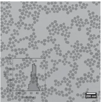
(11) Hassan, P. A.; Rana, S.; Verma, G. Langmuir 2015, 31, 3−12. (12) Bhattacharjee, S. J. Controlled Release 2016, 235, 337−351. Figure 3. TEM micrograph of the silica NPs and the result of the
image analysis. Inset: The probability density function constructed by counting 505 particles. The perimeter-equivalent radius follows a narrow distribution with a mean of 34.1 nm (95% confidence interval for the population mean: 33.8−34.4 nm).
(13) Stetefeld, J.; McKenna, S. A.; Patel, T. R. Biophys. Rev. 2016, 8, 409−427.
(14) Nickel, C.; Angelstorf, J.; Bienert, R.; Burkart, C.; Gabsch, S.; Giebner, S.; Haase, A.; Hellack, B.; Hollert, H.; Hund-Rinke, K.; Jungmann, D.; Kaminski, H.; Luch, A.; Maes, H. M.; Nogowski, A.; Oetken, M.; Schaeffer, A.; Schiwy, A.; Schlich, K.; Stintz, M.; et al. J. Nanopart. Res. 2014, 16, 2260.
(15) Varenne, F.; Botton, J.; Merlet, C.; Beck-Broichsitter, M.; Legrand, F.-X.; Vauthier, C. Colloids Surf., A 2015, 486, 124−138.
(16) Varenne, F.; Botton, J.; Merlet, C.; Hillaireau, H.; Legrand, F. X.; Barratt, G.; Vauthier, C. Int. J. Pharm. 2016, 515, 245−253.
(17) Varenne, F.; Rustique, E.; Botton, J.; Coty, J. B.; Lanusse, G.; Ait Lahcen, M.; Rio, L.; Zandanel, C.; Lemarchand, C.; Germain, M.; Negri, L.; Couffin, A. C.; Barratt, G.; Vauthier, C. Int. J. Pharm. 2017, 528, 299−311.
(18) Yildirimer, L.; Thanh, N. T. K.; Loizidou, M.; Seifalian, A. M. Nano Today 2011, 6, 585−607.
(19) Min, Y.; Caster, J. M.; Eblan, M. J.; Wang, A. Z. Chem. Rev. 2015, 115, 11147−11190.
(20) Krug, H. F.; Wick, P. Angew. Chem., Int. Ed. 2011, 50, 1260− 1278.
(21) Krug, H. F. Angew. Chem., Int. Ed. 2014, 53, 12304−12319. (22) Small, J. A.; Robert, L.; Watters, J. Report of Investigation-Reference Material 8011, National Institute of Standards & Technology: Gaithersburg, MD, 2015.
(23) Meli, F.; Klein, T.; Buhr, E.; Frase, C. G.; Gleber, G.; Krumrey, M.; Duta, A.; Duta, S.; Korpelainen, V.; Bellotti, R.; Picotto, G. B.; Boyd, R. D.; Cuenat, A. Meas. Sci. Technol. 2012, 23, 125005.
(24) Bienert, R.; Emmerling, F.; Thünemann, A. F. Anal. Bioanal. Chem. 2009, 395, 1651.
(25) Yang, H.; Zheng, G.; Li, M.-c. Particle & Particle Systems Characterization 2008, 25, 406−413.
(26) Takahashi, K.; Kato, H.; Saito, T.; Matsuyama, S.; Kinugasa, S. Particle& Particle Systems Characterization 2008, 25, 31−38.
(27) Kwon, S. Y.; Kim, Y.-G.; Lee, S. H.; Moon, J. H. Metrologia 2011, 48, 417.
(28) Kowalczyk, B.; Lagzi, I.; Grzybowski, B. A. Curr. Opin. Colloid Interface Sci. 2011, 16, 135−148.
(29) Stock, R. S.; Ray, W. H. J. Polym. Sci., Polym. Phys. Ed. 1985, 23, 1393−1447.
(30) Koppel, D. E. J. Chem. Phys. 1972, 57, 4814−4820. (31) Frisken, B. J. Appl. Opt. 2001, 40, 4087−4091.
(32) Hassan, P. A.; Kulshreshtha, S. K. J. Colloid Interface Sci. 2006, 300, 744−748.
(33) Mailer, A. G.; Clegg, P. S.; Pusey, P. N. J. Phys.: Condens. Matter 2015, 27, 145102.
(34) Geers, C.; Rodriguez-Lorenzo, L.; Andreas Urban, D.; Kinnear, C.; Petri-Fink, A.; Balog, S. Nanoscale 2016, 8, 15813−15821.
(35) Provencher, S. W. Comput. Phys. Commun. 1982, 27, 229−242. (36) Scotti, A.; Liu, W.; Hyatt, J. S.; Herman, E. S.; Choi, H. S.; Kim, J. W.; Lyon, L. A.; Gasser, U.; Fernandez-Nieves, A. J. Chem. Phys. 2015, 142, 234905.
(37) Zhu, X.; Shen, J.; Liu, W.; Sun, X.; Wang, Y. Appl. Opt. 2010, 49, 6591−6596.
(38) Shen, J.; Thomas, J. C.; Zhu, X.; Wang, Y. Opt. Express 2011, 19, 12284−12290.
(39) Zhu, X.; Shen, J.; Thomas, J. C. Appl. Opt. 2012, 51, 7537− 7548.
(40) Mao, S.; Shen, J.; Thomas, J. C.; Zhu, X.; Liu, W.; Sun, X. Appl. Opt. 2012, 51, 6220−6226.
(41) Wang, Y.; Shen, J.; Wei, L.; Dou, Z.; Gao, S. Appl. Opt. 2013, 52, 2792−2799.
(42) Roger, V.; Cottet, H.; Cipelletti, L. Anal. Chem. 2016, 88, 2630− 2636.
(43) Nyeo, S. L.; Chu, B. Macromolecules 1989, 22, 3998−4009. (44) Livesey, A. K.; Licinio, P.; Delaye, M. J. Chem. Phys. 1986, 84, 5102−5107.
(45) Nyeo, S.-L.; Ansari, R. R. Journal of Computational and Applied Mathematics 2011, 235, 2861−2872.
(46) Clementi, L. A.; Vega, J. R.; Gugliotta, L. M. Particle& Particle Systems Characterization 2010, 27, 146−157.
(47) Clementi, L. A.; Vega, J. R.; Orlande, H. R. B.; Gugliotta, L. M. Inverse Probl. Sci. Eng. 2012, 20, 973−990.
(48) Nyeo, S.-L.; Ansari, R. R. Laser Phys. 2015, 25, 075703. (49) Gugliotta, L. M.; Stegmayer, G. S.; Clementi, L. A.; Gonzalez, V. D. G.; Minari, R. J.; Leiza, J. R.; Vega, J. R. Particle& Particle Systems Characterization 2009, 26, 41−52.
(50) Ford, N. C. Light Scattering Apparatus. In Dynamic Light Scattering-Applications of Photon Correlation Spectroscopy; Pecora, R., Ed.; Springer: New York, 1985; pp 7−58.
(51) Licinio, P.; Delaye, M. J. Phys. Chem. 1987, 91, 231−235. (52) Ruf, H. Langmuir 2002, 18, 3804−3814.
(53) Haller, H. R.; Destor, C.; Cannell, D. S. Rev. Sci. Instrum. 1983, 54, 973−983.
(54) Goodman, J. W. Statistical Optics; Wiley: New York, 2000. (55) Bossert, D.; Natterodt, J.; Urban, D. A.; Weder, C.; Petri-Fink, A.; Balog, S. J. Phys. Chem. B 2017, 121, 7999−8007.
(56) Yazici, B.; Yolacan, S. Journal of Statistical Computation and Simulation 2007, 77, 175−183.
(57) Shapiro, S. S.; Wilk, M. B. Biometrika 1965, 52, 591.
(58) Yap, B. W.; Sim, C. H. Journal of Statistical Computation and Simulation 2011, 81, 2141−2155.
(59) International Organization for Standardization. Particle Size Analysis-Dynamic Light Scattering (DLS), ISO 22412:2017; Interna-tional Organization for Standardization: Geneva, Switzerland, 2017.