Holzforschung 2015; 69(7): 839–849
*Corresponding author: Dominique Derome, Laboratory for Multiscale Studies in Building Physics, Empa, Switzerland, Uberlandstrasse 129, Dübendorf, e-mail: [email protected]
Saeed Abbasion: Department of Civil Engineering, ETHZ, Switzerland
Peter Moonen: Université de Pau et des Pays de l’Adour (UPPA), Pau, France
Jan Carmeliet: Chair of Building Physics, ETHZ, Switzerland; and Laboratory for Multiscale Studies in Building Physics, Empa, Switzerland
Saeed Abbasion, Peter Moonen, Jan Carmeliet and Dominique Derome*
A hygrothermo-mechanical model for wood:
Part B. Parametric studies and application
to wood welding
COST Action FP0904 2010–2014: Thermo-Hydro-Mechanical wood behavior and processing
Abstract: The correct prediction of the behavior of woodcomponents undergoing environmental loading or indus-trial process requires that the hygric, thermal and mechan-ical (HTM) behavior of wood are considered in a coupled manner. A fully coupled poromechanical approach has been used to perform a parametric study on wood HTM behavior, and the results have been validated with neu-tron imaging measurements on a moist wood specimen exposed to high temperature. Further, HTM behavior of wood during welding has been simulated by the model. For such a simulation, proper material properties are needed, as some of them, for example thermal conductiv-ity, have a significant influence on the local and temporal behavior of the material.
Keywords: heat and mass transport, hygrothermal and
mechanical behavior, poromechanics, wood
DOI 10.1515/hf-2014-0190
Received June 30, 2014; accepted April 20, 2015; previously pub-lished online May 14, 2015
Introduction
Wood as a traditional building material is well character-ized in terms of its hygric, thermal and mechanical (HTM) properties (Kollmann and Côté 1968) and the role of these properties on timber quality is also known (Siau 1984;
Skaar 1998). Mathematical methods to predict and quan-tify heat and mass transport in wood under different envi-ronmental conditions have also been developed (Plumb et al. 1985; Turner 1996; Perré and Turner 2002; Defo et al. 2004; Rémond et al. 2007). Nowadays, wood and wood-based materials are still in focus as renewable and environmentally friendly materials. New techniques and methods were developed for the modification and assem-bly of wood for industrial use. One of such methods is welding, in the course of which wood samples are submit-ted for a few seconds to friction vibration where tempera-tures higher than 200°C may develop between the wood pieces. The thin layer formed by pyrolytic/ thermoplastic modification acts as adhesive. From the practical and the-oretical point of view, it would be desirable to model math-ematically this process and other HTM property changes. The full characterization of the material properties for the temperature range of interest is time consuming and thus computational parametric studies and sensitivity analyses are useful to identify the most impacting material proper-ties and factors. In this context, Olek et al. (2003) studied the effect of thermal conductivity on modeling accuracy and Younsi et al. (2010) the effects of the convective trans-fer coefficients on the mass and heat transtrans-fer fields in the material. In the field of high- temperature modeling of wood, reliable data are not yet available.
In the present paper, parametric studies on common hygric and thermal properties at different temperatures will be presented in the context of wood welding. A special focus will be on the poromechanical approach in which the complex HTM behavior of wood will be con-sidered in a fully coupled manner (Abbasion et al. 2015). The transport of heat and mass will be described based on temperature and pressure gradients as the driving forces. For mass transfer, distinction has to be made between the liquid and the gas phase while both are driven by corre-sponding pressure differences. A continuum approach is retained, where the different phases are considered to be superimposed at each point in the material. The process will be analyzed at the macroscopic scale, where neither
the different material components nor the cellular struc-ture of the wood can be distinguished. The boundary con-ditions and the numerical domain will be presented for the parametric study and for welding. Finally the results concerning the material properties and the welding simu-lation will be presented.
Boundary conditions and numerical
domain
Parametric study
The dimensions of the wood sample are 40 (height) × 80 (width) × 10 (thickness) mm3, i.e., the same as described
by Abbasion et al. (2015) for a neutron transmission radi-ography study. Given symmetry, the calculation domain covers half of the specimen. In addition, to reduce the simulation time, the problem is considered to be two-dimensional (2D), assuming that the transport in the third direction is negligible. The wood sample is divided into several growth rings. Each ring has 3 mm width with an average density of 376 kg m-3, with 2.4 mm of
early-wood (EW) at 300 kg m-3 and 0.6 mm of latewood (LW)
at 680 kg m-3. For simplicity, all growth rings have 3 mm
width, where the EW/LW ratio is 4:1. As seen in Figure 1a, a constant temperature, Tbase, is applied at the bottom of the sample. For the symmetry plane, adiabatic bound-ary conditions for heat and no mass transfer are imple-mented. At the right and top boundaries, which are in contact with the environment, convective heat and mass transfer occurs.
Application to wood welding
Thermally and mechanically, the process can be described by three phases. Phase 1: Due to the Coulomb friction resistance at the interface of the two samples rubbing against each other, temperature (T) increases rapidly and a sharp T gradient develops across the first 2 mm of wood from the interface. The high T and sharp T gradient force the free and adsorbed water phase to be transported downstream of the heat flux. In the range of 80–100°C, lignin softens and becomes rubber-like. The exothermic hydrolysis of hemicelluloses starts at 110°C and hydroly-sis of paracrystalline cellulose occurs above 140°C. With increasing T, several hydrolysis and condensation reac-tions of sugar monomers take place. From 190°C, the pyrolysis of hemicelluloses and cellulose begins, which
40 mm
Convective heat and mass transfer
2.4 mm 3.0 mm L R Symmetry plane Y Z Y Z (L) 2l 2b h X P1 P2 Y X θ T R P1 P2 Symmetry plane Symmetry plane Earlywood 40 mm Latewood ρ=300 kg m-3ρ=680 kg m-3 a b
Figure 1: Computational domain and corresponding boundary conditions, a) for the parametric studies, b) for the welding process parametric studies with a 3D schematic representation of two wood samples in contact, and the orientation of the two planes of reference.
is accompanied by the hydrolysis of lignin above 200°C. The complex chemical reactions are described by Ganne-Chédeville et al. (2008). During this phase, the density of a thin layer of the interface ( < 1 mm) increases by a factor ≈1.5. The displacement rate of the welded plane is con-stant. Phase 2: In this phase, T is constant and the normal displacement continues steadily and at a higher rate than before. Above 225°C, depolymerization of the crystalline cellulose begins. At the interface, the conditions are very close to pyrolysis temperature, but the reactions are slow due to the lack of oxygen (Ganne-Chédeville et al. 2008).
Phase 3: The machine vibration is stopped but the
pres-sure is maintained and the sample cools down under pressure. An example of the variation of the parameters displacement, friction coefficient and temperature during the three welding phases is depicted in Figure 2a (see also Stamm 2005).
S. Abbasion et al.: Hygrothermo-mechanical model for wood: Part B 841
To reduce simulation time, the welding process is modeled in 2D and the growth rings are simplified to a bi-layered composite material. The welding of two identical wood pieces is assumed, which are described by three sym-metry planes (Figure 1b). Planes 1 and 2, corresponding to the RT and LT planes, are selected for 2D simulation, each plane having one side adiabatic and impermeable to moisture (M). As the results are very similar, only the results for 1 are presented.
The heat generation at the interface of two samples is modeled as an equivalent heat source based on friction force measurement (Stamm 2005) and data from Ganne-Chédeville et al. (2008). Figure 2b is reproduced from the
latter and shows the measured heat flux during the linear welding of beech wood (Fagus sylvatica L.) for three differ-ent welding times. In the following, the conditions in Figure 2 are referred to as the welding boundary conditions.
Parametric study on material
properties
In this parametric study on material properties, param-eters considered consist of liquid and gas intrinsic perme-ability Kl and Kg, respectively, vapor diffusion coefficient
Figure 2: a) Typical diagram of the temperature, friction coefficient at the interface of the welded samples and the vertical displace-ment of the press (Stamm 2005), b) typical heat flux at the interface of two samples (Ganne-Chédeville et al. 2008) and corresponding boundary conditions for 2D simulation.
Figure 3: Results of modeling. Average MCs vs. time at the dis-tances from the weld line indicated (a–d), MCmax and its location
(e–f) and temperature vs. time (g–h) in cases of different intrinsic permeability (Z).
Dg, thermal conductivity λ, and fiber saturated moisture
content (MC) as a function of temperature, MCsat(T), which are characterized, at least in part, in many experimental works (Kühlmann 1962; Weichert 1963; Kuroda and Siau 1988; Zillig 2009; Sonderegger et al. 2011).
Effects of the liquid and gas intrinsic
permeability
The intrinsic permeability presents some uncertainty as it can vary over four orders of magnitude. The impact of varying the liquid and gas intrinsic permeability is studied with:
=10Z 0, =10Z 0
l l g g
K K K K (1)
where Z is an integer from -4 to 2, and superscript 0 refers
to the base value. A sample at equilibrium with 80% RH is exposed to 150°C for 30 minutes for transport in the radial-longitudinal (RL) plane. Graphs of MC vs. time at four heights for seven cases of intrinsic permeability,
plus one case without gas permeability are presented in Figure 3a–d and of magnitude and location of maximum MC vs. time in Figure 3e–f. Increasing the permeability increases the maximum MC (MCmax) reached, but short-ens the duration of the MC peak. Increasing permeabil-ity above its reference value has almost no effect, while reducing it leads to a longer presence of M within the base of the sample and delays its transport towards the top of the sample. As a result, the MC peak during the heating process is closer to the sample base with decreasing permeability (Figure 3f). Increasing the material perme-ability elevates the rate of the M penetration and its mag-nitude. The magnitude of MCmax reaches rapidly a steady state between 17 and 19%, for low and high permeability, respectively. It seems that accurate experimental M pro-files could allow identifying the order of magnitude of the permeability term.
The effect of the permeability on the T distribu-tion inside the sample is less important, as shown in Figure 3g–h. The thermal conductivity of the wood increases with increasing MC. The sample with lower permeability retains more M at the bottom and, as a
Figure 4: Average moisture content vs. time with initial MCs of a) 26%, b) 14.5%, c) 7.5%, d) 2.5% at four heights. Solid and dotted lines for the results of simulation with and without considering the gas pressure, respectively.
S. Abbasion et al.: Hygrothermo-mechanical model for wood: Part B 843
consequence, has a higher thermal conductivity. The order of the curves changes with increasing height, prob-ably due to the M redistribution and its effect on local thermal conductivity and capacity.
In Figure 3, the calculations are performed with and without gas transport. In the latter case the data are close to the results of very high permeability. To explore this further, the same situation is modeled with four differ-ent initial MCs, namely MC0 = 2.5, 7.5, 14.5, and 26%, which are related to equilibrium with RHs 10, 50, 80, and 99% at 25°C. In porous media, the heated moist air builds a pres-sure that will contribute to flow amplification, i.e., to mass transport. The simulations with and without considering gas pressure are presented in Figure 4. Decreasing the initial MC results in sharper MC profiles. For samples with
low MC, the gas pressure has almost no effect on the M transport. The effect of the advection term is more obvious at higher MC, i.e., in the regions where both adsorption and desorption are effective during heating, which corre-sponds to the heights of 5 and 10 mm of the sample.
Effects of vapor diffusion coefficient
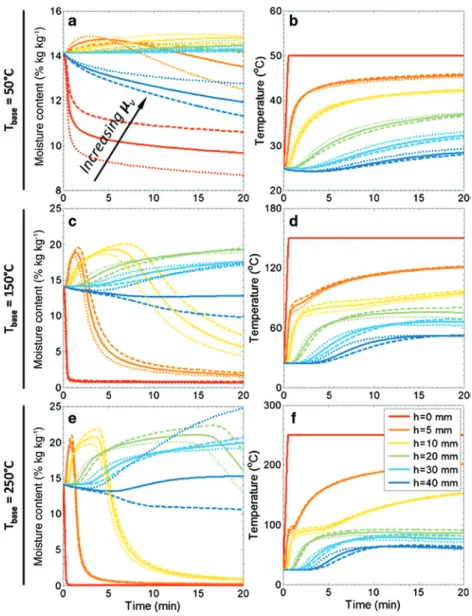
The effect of varying the vapor diffusion coefficient on the heat and mass transport is studied with three imposed base temperatures, i.e., Tbase 50, 150, and 250°C. The vapor resistance factor μv, which is proportional to the inverse of the vapor diffusion coefficient Dg, is varied by multiplying
it with a scaling factor d:
Figure 5: Moisture content and temperature vs. time at different heights in the sample. Dashed-line is for the case d = 2.0, solid-line for
= 0
v d v
µ µ (2)
where d is 0.5, 1, or 2.
The MC and T at six positions along the height of the sample are plotted vs. time for the three Tbase and the three vapor resistance factors (Figure 5). Changing the value of μv has a significant effect on the M distri-bution near the heating source, at 150°C and even more at 50°C where, the rate of drying reduces noticeably by increasing the vapor resistance factor. By increasing the
Tbase, the effect of the μv change near the heating source decreases and becomes more important in the top half of the sample, far away from the heat source. The lower μv results in easier penetration of the water vapor in the material. In contrast, the T profiles are not as sensitive to
the change of μv. However, the effect is mainly noticeable in the top half of the samples.
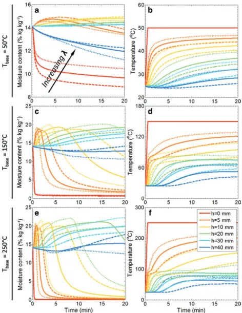
Effects of thermal conductivity
When considering the thermal conductivity, λ, the thermal conductivity tensor is scaled by a scalar λ̅,
λ =
λ λ (3)
with the scaling factor λ̅ equals to 0.5, 1.0, or 2.0. The three
Tbase are the same as in the previous paragraph.
Figure 6 presents the MC and T vs. time plots for the three Tbase and the three scaling factors, for six locations along the sample height. As it is seen in the first column,
Figure 6: Moisture content and temperature at different heights in the sample. Dashed-line is for the case λ= 2.0, solid-line for λ= 1.0 and dotted-line is λ= 0.50.
S. Abbasion et al.: Hygrothermo-mechanical model for wood: Part B 845
Modeling the welding of wood
process
In this section, the heat and mass transfer in the wood samples during the welding process is modeled, illus-trating how numerical results can provide insights in the welding process. The initial MC of wood and its effect on the T distribution at and near the interface of the two specimens are considered. This parameter is selected because, in practice, the initial MC is easily controllable without much additional expenses for wood pre-conditioning.
Spruce wood was considered in the P1 plane and with a cross section of b × h = 25 × 10 mm2. The selected initial
MCs are 0.14, 12.8 and 28%. The heat flux selected cor-responds to 4.5 s welding as given by Ganne-Chédeville et al. (2008) (Figure 2b). The air conditions are 100 kPa, varying λ has a significant influence on the M transport
inside the medium. This effect is present for all three Tbase ranges and at all heights, except in the top half of the sample exposed to 50°C at its base. In terms of Tbase dis-tribution in the sample, as seen in the second column of Figure 6, the effect of λ becomes more and more important with increasing Tbase. In terms of this parameter, all the regions inside the medium and during the total heating time are considerably affected (which was not the case for μv). Thermal conductivity plays a significant role on the rate and amount of M and heat transport in porous media. Erroneous assumption in this regard will largely affect the simulation prediction.
Effect of the fiber saturation moisture
content
The fiber saturation MC as a function of temperature, Mcsat(T), has a high practical importance. According to literature, MCsat decreases by 0.1% per 1°C incre-ment (Weichert 1963; Siau 1984; Skaar 1998). However, most of the available data are for the range 100–150°C. MCsat at higher T is normally not measured but simply extrapolated. Thus, it is of interest to know how strongly this approximation affects the M and T fields. Hence, Gaussian type functions will be applied to predict MCsat vs.
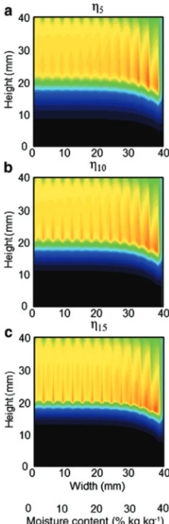
T curves, with a MCsat at 100°C that is 5, 10 or 15% less than the MCsat at room temperature, referred to as η5, η10 and η15. The calculation shows that the T dependency of MCsat has a small effect on the overall behavior of the material and its effect is discernable only in the last stages of drying. By heating the material, the RH decreases in the regions near the heat source, leading to the desorption of M until a new equilibrium is reached. The variation of MCsat results in a slight variation of the sorption curves, thus resulting in the slight variation of MC observed. Because of these differences in the drying, the regions at a larger distance from the heat source receive different amounts of water vapor and the plateauing of the curves is delayed. In par-allel, an impact on the T curves is not discernable.
To illustrate the influence of MCsat(T) on M transport at mesoscale, MC contours are plotted in Figure 7 for the three cases at 20 min. Although the average MCs at dif-ferent heights are almost the same, as mentioned above, going from η5 to η15 results in the narrowing of the transi-tion zone between the dry and wet zones. Transport occurs mainly in the direction of the heat flux propagation, i.e., along the growth ring direction, rather than the transverse direction, across the rings, resulting in the appearance of sharper boundaries for EW and LW MC distribution.
Figure 7: MC distribution inside the sample for different fiber satu-ration moisture profiles at t = 20 min.
Figure 8: Time history of the average temperature, gas pressure and MC at some selected heights in the wood specimens with initial MCs of 0.14, 12.8, and 28.0% and welding time of t = 4.5 s.
25°C and 50% RH. Since in this example the deformation of the sample is not taken into account, no value is allo-cated to the applied pressure during welding. In Figure 8, the average T, gas pressure and MC are plotted vs. time at nine locations along the sample height. These average values are calculated along the first 5 mm from the left symmetry line. With increasing initial MC, the peak of the T profiles lowers. This is due to the fact that a part of
the energy is consumed by the heating and phase change of water. This is confirmed in the gas pressure profiles where higher starting MC results in increased gas pres-sure inside the sample. The gas prespres-sure at the interface,
h = 0.0 mm, increases by a factor of 2 for sample MC0.14 and by a factor 5 for sample MC12.8. However, the magnitude of the peak in gas pressure is not directly correlated to the MC. Due to the low permeability of wood in the transverse
S. Abbasion et al.: Hygrothermo-mechanical model for wood: Part B 847
directions and the low welding time, M does not pene-trate too much the sample interior, as shown in the third row of Figure 8. For the MC12.8 and MC28.0 cases, the MC within 2 mm of the weld line is greater than the fiber satu-ration point (FSP).
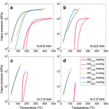
The effect of initial MC on vapor generation was studied at four heights in the sample where vapor pressure is plotted as a function of T in Figure 9. The plots in this figure are divided into heating and cooling parts, where the former corresponds to the welding time, 0 ≤ t ≤ 4.5 s, and the latter to the time after stopping the vibrational movement, 4.5 < t ≤ 60 s. Although the MC12.8 sample reaches a higher T and consequently a higher vapor pres-sure than the MC28.0, the vapor pressure changes induced by a T increment have the same trend for both of them in the heating phase. In the cooling phase, the vapor pres-sure has lower values at the same T for the points near the weld line due to the vapor transfer from these regions further away. These heating and cooling phases describe a hysteresis-like loop in the T-vapor pressure plane which becomes narrower with increasing distances from the heat source. The widths of these loops are corresponding to the evaporation/condensation rate and vapor permeability of the medium. For the dry sample, MC0.14, the vapor pressure becomes considerable above 150°C.
Figure 10 is a plot, where the distribution of T, gas pressure and M distribution along the height of the
Figure 9: Average vapor pressure vs. temperature at some selected heights in the wood specimens with initial MCs of 0.14, 12.8 and 28.0% and welding time of t = 4.5 s.
samples are recorded vs. time for the first 4 mm from the weld line. As seen, the depth of penetration at T > 300°C is very low and < 1 mm deep for the dry sample and around 200–300 μm for the moist samples. The gas pressure dis-tribution inside the sample exhibits a similar trend to what is seen in the T plots, although gas pressure varia-tions penetrate further inside the sample. The penetration depth of the gas inside the sample decreases with increas-ing initial MC, which is due to both the lower Tbase, in case of the same heating flux, as well as the higher specific heat of the specimens in case of higher initial MCs, which causes vapor flow to condense faster inside the sample. During welding time, M gathers locally in front of the high pressure resulting from the high evaporation rate. This moist region redistributes during the cooling phase and a portion flows back to the welded zone. However, in the real welding process, chemical degradation happens and the hygric properties will be different. Thus, consid-erations based on non-degraded wood, as done here, may give inaccurate results.
Welding time is one of the most important control-ling parameters of the process and an approach will be presented for the estimation of this parameter. As T is the main factor in this context, isotherms can be plotted as a function of sample position, and time for selected T. By increasing the selected T or initial MC, the time which is needed for reaching a set T increases; it may also occur that the desired T cannot be reached. For example, in Figure 11, a horizontal line is drawn at the height of 0.5 mm from the weld line. This line intersects the lines related to 200°C at 2.68 and 4.35 s corresponding to MC0.14 and MC12.8, respectively, and does not intersect the MC28.0 curve. These times are in good agreement with the selected welding time for the spruce wood determined by Stamm (2005) which are 3.1, 5.4 and 7.5 s for the MC0.14, MC12.8 and MC28.0, respectively. Thus, this approach shows that the selected welding time is not long enough for the sample with initial MC of 28%. It seems that studying the temperature pen-etration time could be a promising method to approximate the proper welding time.
Conclusion
The results of the parametric study presented above revealed that a mathematically complete model should be supported with accurate material properties to grant accurate and realistic results. Without experimental data, careful sensitivity analysis is necessary to assess the complex interrelation of the data. In the case of the liquid/
gas bulk conductivity, the importance of the parameters is limited. On the other hand, the thermal conductivity influences significantly the local and temporal behav-ior of the material. Generally speaking, the temperature field is more stable and insensitive concerning material properties changes than the moisture content field is. Nevertheless, variations of the thermal properties have a larger influence on the material behavior then the hygric properties.
The modeling results, with large practical impor-tance, seem to be appropriate, though the wood welding process is very complex. Despite several simplifications and assumptions, the insights delivered by the model are valuable. Thus modeling can be used to support experi-mental and numerical studies.
One of the major underlying assumptions of the pro-posed model is that of local thermal equilibrium, i.e., that all three phases in the porous material at a local point have the same temperature. This assumption remains to be verified for very fast processes. This assumption also implies that microscale heat transfer effects are not significant at the macroscale. The mechanical effects on the transport properties, which could have a significant influence near the weld line, have not been considered in the model. In a more general model, the kinetics of chemical reactions such as carbon dioxide generation or material changes, including plastic deformation, should also be included into the model. This will certainly have an effect on the moisture and heat transport in the material.
Figure 10: Distribution of the average temperature, gas pressure and MC along the first 4 mm height of the wood specimens with initial MCs of 0.14, 12.8, and 28.0% and welding time of t = 4.5 s.
S. Abbasion et al.: Hygrothermo-mechanical model for wood: Part B 849 during linear welding using the finite element method. J Adhes. Sci. Technol. 22:1209–1221.
Kollmann, F.P., Côté, W.A. Principles of Wood Science and Technol-ogy. Vol. I. Solid wood, Springer-Verlag, Berlin, Heidelberg, New York, 1968.
Kühlmann, G. (1962) Investigation of the thermal properties of wood and particleboard in dependency on moisture content and temperature in the hygroscopic range. Holz Roh Werkst. 20:259–270.
Kuroda, N., Siau, J.F. (1988) Evidence of nonlinear flow in softwoods from wood permeability measurements. Wood Fiber Sci. 20:162–169.
Olek, W., Weres, J., Guzenda, R. (2003) Effects of thermal conduc-tivity data on accuracy of modeling heat transfer in wood. Holzforschung 57:317–325.
Perré, P., Turner, I.W. (2002) A heterogeneous wood drying compu-tational model that accounts for material property variation across growth rings. Chem. Eng. J. 86:117–131.
Plumb, O.A., Spolek, G.A., Olmstead, B.A. (1985) Heat and mass transfer in wood during drying. Int. J. Heat Mass Tran. 28:1669–1678.
Rémond, R., Passard, J., Perré, P. (2007) The effect of temperature and moisture content on the mechanical behaviour of wood: a comprehensive model applied to drying and bending. Eur. J. Mech. A-Solid. 26:558–572.
Siau, J.F. Transport Processes in Wood. Springer-Verlag, Germany, 1984.
Skaar, C. Wood-Water Relations. Springer-Verlag Berlin, Germany, 1998.
Sonderegger, W., Hering, S., Niemz, P. (2011) Thermal behaviour of Norway spruce and European beech in and between the princi-pal anatomical directions. Holzforschung 65:369–375. Stamm, B. Development of friction welding of wood – physical,
mechanical and chemical studies. Doctoral Thesis EPF Laus-anne, IBOIS, 187 pages, 2005.
Turner, I.W. (1996) A two-dimensional orthotropic model for simulating wood drying processes. Appl. Math. Model. 20:60–81.
Weichert, L. (1963) Investigations on sorption and swelling of spruce, beech and compressed-beech wood at temperatures between 20 and 100°C. Holz Roh Werkst. 21:290–300. Younsi, R., Kocaefe, D., Poncsak, S., Kocaefe, Y., Gastonguay, L.
(2010) A high-temperature thermal treatment of wood using a multiscale computational model: application to wood poles. Biores. Technol. 101:4630–4638.
Zillig, W. Moisture transport in wood using a multiscale approach. PhD thesis. Katholieke Universiteit Leuven, Leuven, Belgium, 2009.
Acknowledgments: SNF Sinergia grant no. 127467 and
the COST Action FP0904 of the EU RTD Framework Pro-gramme are acknowledged.
References
Abbasion, S., Carmeliet, J., Sedighi Gilani, M., Vontobel, P., Derome, D. (2015) A hygrothermo-mechanical model for wood: Part A. Poroelastic formulation and validation with neutron imaging – COST Action FP0904 2010–2014: Thermo-hydro-mechanical wood behavior and processing. Holzforschung 69:825–837.
Defo, M., Fortin, Y., Cloutier, A. (2004) Modeling superheated steam vacuum drying of wood. Dry Technol. 22:2231–2253.
Ganne-Chédeville, C., Duchanois, G., Pizzi, A., Leban, J.-M., Pichelin, F. (2008) Predicting the thermal behaviour of wood Figure 11: Time-based isotherms of the average temperature along the height of the wood specimens with initial MCs of 0.14, 12.8, and 28.0% and welding time of t = 4.5 s at three selected temperatures.