HAL Id: hal-01968126
https://hal.archives-ouvertes.fr/hal-01968126
Submitted on 2 Jan 2019
HAL is a multi-disciplinary open access
archive for the deposit and dissemination of
sci-entific research documents, whether they are
pub-lished or not. The documents may come from
teaching and research institutions in France or
abroad, or from public or private research centers.
L’archive ouverte pluridisciplinaire HAL, est
destinée au dépôt et à la diffusion de documents
scientifiques de niveau recherche, publiés ou non,
émanant des établissements d’enseignement et de
recherche français ou étrangers, des laboratoires
publics ou privés.
characterize auto- and heterotrophic plankton
communities
Monique Messié, Igor Shulman, Severine Martini, Steven H.D. Haddock
To cite this version:
Monique Messié, Igor Shulman, Severine Martini, Steven H.D. Haddock. Using fluorescence and
bioluminescence sensors to characterize auto- and heterotrophic plankton communities. Progress in
Oceanography, Elsevier, 2019, 171, pp.76-92. �10.1016/j.pocean.2018.12.010�. �hal-01968126�
Contents lists available atScienceDirect
Progress in Oceanography
journal homepage:www.elsevier.com/locate/poceanUsing fluorescence and bioluminescence sensors to characterize auto- and
heterotrophic plankton communities
Monique Messié
a,b,⁎, Igor Shulman
c, Séverine Martini
d, Steven H.D. Haddock
aaMonterey Bay Aquarium Research Institute, Moss Landing, CA 95039, USA
bAix Marseille Univ., Université de Toulon, CNRS, IRD, MIO UM 110, 13288 Marseille, France cUS Naval Research Laboratory, Stennis Space Center, MS 39529, USA
dSorbonne Université, CNRS, Laboratoire d’Océanographie de Villefranche, LOV, F-06230 Villefranche-sur-mer, France
A R T I C L E I N F O Keywords: Bioluminescence Fluorescence Phytoplankton Zooplankton Coastal upwelling Time series A B S T R A C T
High-resolution autonomous sensors routinely measure physical (temperature, salinity), chemical (oxygen, nutrients) and biological (fluorescence) parameters. However, while fluorescence provides a proxy for phyto-plankton, heterotrophic populations remain challenging to monitor in real-time and at high resolution. Bathyphotometers, sensors which measure the light emitted by bioluminescent organisms when mechanically stimulated, provide the capability to identify bioluminescent dinoflagellates and zooplankton. In the coastal ocean, highly abundant dinoflagellates emitting low-intensity flashes generate a background bioluminescence signal, while rarer zooplankton emit bright flashes that can be individually resolved by high-frequency sensors. Bathyphotometers were deployed from ships and onboard autonomous underwater vehicles (AUVs) during three field campaigns in Monterey Bay, California. Ship-based in situ water samples were simultaneously collected and the plankton communities characterized. Plankton concentrations were matched with concurrent datasets of fluorescence and bioluminescence to develop proxies for autotrophic and heterotrophic dinoflagellates, other phytoplankton such as diatoms, copepods, larvaceans (appendicularians), and small jellies. The method extracts the bioluminescence background as a proxy for dinoflagellates, and exploits differences in bioluminescence flash intensity between several types of zooplankton to identify larvaceans, copepods and small jellies. Fluorescence is used to discriminate between autotrophic and heterotrophic dinoflagellates, and to identify other autotrophic plankton. Concurrent fluorometers and bathyphotometers onboard AUVs can thus provide a novel view of plankton diversity and phytoplankton/zooplankton interactions in the sea.
1. Introduction
Autonomous platforms such as profiling floats, gliders or autono-mous underwater vehicles (AUVs) have revolutionized oceanography by providing high-resolution, continuous measurements across the water column. In the field of biological oceanography, the early in-tegration of fluorometers onboard autonomous platforms have pro-vided unprecedented views of phytoplankton structure and variability in the upper ocean (e.g.,Mahadevan et al., 2012; Rudnick, 2016). Other biological sensors have been integrated into gliders and AUVs in recent years, targeting zooplankton, fish, and larger animals using acoustic backscatter (Powell and Ohman, 2012) and echo sounders (Moline et al., 2015). Despite these advances, the characterization of biological communities remains elusive, particularly for small plankton. Most optical and acoustic sensors only measure bulk properties and cannot distinguish between taxonomic groups, although ratios of fluorescence
to optical backscatter have been shown to correlate with phytoplankton community composition (Cetinić et al., 2015). Recent advances using spectral fluorescence show promise in characterizing phytoplankton community composition (Richardson et al., 2010) but have not yet been integrated onboard autonomous platforms to our knowledge. Imaging and ecogenomic sensors targeting phytoplankton and zooplankton provide taxonomic information but come with their own set of chal-lenges, such as power requirements, size, data telemetry, environment, and cost (Lopez et al., 2015).
In the family of biological autonomous sensors, bathyphotometers (sensors which measure the light emitted by small bioluminescent or-ganisms when mechanically stimulated) are at the intersection between “bulk” and “taxon-specific” sensors. Bioluminescence as measured by a bathyphotometer is a bulk property that scales with biomass for a given planktonic community (Lapota, 1998; Latz and Rohr, 2013). In addi-tion, characteristics of bioluminescent emissions such as flash shape,
https://doi.org/10.1016/j.pocean.2018.12.010
Received 23 February 2018; Received in revised form 12 December 2018; Accepted 13 December 2018
⁎Corresponding author.
E-mail address:monique@mbari.org(M. Messié).
Available online 14 December 2018
0079-6611/ © 2018 The Authors. Published by Elsevier Ltd. This is an open access article under the CC BY-NC-ND license (http://creativecommons.org/licenses/BY-NC-ND/4.0/).
duration and intensity (hereafter flash kinetics) are taxon-specific and can be used to discriminate between taxa either directly (Johnsen et al., 2014) or via their impact on time series properties (Moline et al., 2009). Bioluminescence is very common throughout the water column, with 76% of marine animals observed at depths between 100 and 4000 m off California (planktonic or not) having bioluminescent capability (Martini and Haddock, 2017). In the upper ocean, small plankton communities include several bioluminescent species (Fig. 1); the most commonly encountered bioluminescent organisms are dinoflagellates (auto- and heterotrophic). Other bioluminescent taxa include larva-ceans (appendicularians), copepods, euphausiids (krill), and small jel-lies (ctenophores and small medusae) (Haddock et al., 2010); their concentrations are typically 2–3 orders of magnitude less than for bioluminescent dinoflagellates (Fig. 1).
Because of the variety of bioluminescent species spanning phyto-plankton (autotrophic dinoflagellates), small heterotrophic protists (heterotrophic dinoflagellates, radiolarians) and zooplankton (cope-pods, krill, and small gelatinous zooplankton), bathyphotometers pre-sent a unique opportunity to study plankton communities, their taxo-nomic composition and phytoplankton/zooplankton interactions in the sea. Efforts to move beyond bulk bioluminescence and to partition bioluminescence into taxonomic groups include light budgets, which require coinciding plankton counts (e.g., Marcinko et al., 2013a; Lapota, 2012a, 2012b), taxon discrimination using flash kinetics (Johnsen et al., 2014; Cronin et al., 2016) and time-series analysis (Moline et al., 2009). In coastal regions where the concentration of bioluminescent organisms is often high enough that flashes merge and become indistinguishable, methods based on flash kinetics cannot be
used. To overcome this issue, here we propose a novel time series analysis method that exploits differences in concentration and flash intensity between taxa to define bioluminescence proxies for dino-flagellates, copepods, larvaceans, and small jellies. Combined with si-multaneous measurements of fluorescence, these proxies can be ex-tended to characterize communities of autotrophic and heterotrophic dinoflagellates, and other phytoplankton such as diatoms.
The paper is organized as follows.Section 2presents the fluores-cence and bioluminesfluores-cence datasets, a modeling exercise used to in-vestigate the impact of concentration and flash kinetics on the biolu-minescence signal, the proxy calculation method, and its application to three field campaigns during which in situ plankton counts were col-lected alongside matching fluorescence/bioluminescence time series. Section 3validates the proxies against in situ counts and presents results during the AOSN-2003 field campaign.Section 4 discusses situations when proxies may or may not be valid, and conclusions are offered in Section 5.
2. Datasets and methods
2.1. Fluorescence and bioluminescence sensors
The plankton proxies are based on bioluminescence and fluores-cence measured by autonomous sensors onboard AUVs or deployed from ships. Bioluminescence and fluorescence are both light emissions by organisms, the main difference being that bioluminescence is pro-duced by the organism itself through a chemical reaction, while fluor-escent molecules do not produce their own light but absorb and reemit
Fig. 1. Average bioluminescent plankton community composition measured during three field campaigns in Monterey Bay, California (top: phytoplankton, bottom:
zooplankton). Field campaigns and sampling are described inSection 2.5. Samples are separated between surface (shallower than 20 m) and subsurface (below 20 m). The numbers of corresponding samples are given on top of each bar; there are more zooplankton than phytoplankton samples available. Species identified as Ceratium
lineatum during MUSE-2000 were removed from the Ceratium counts shown here because that species is non bioluminescent; most Ceratium species were not
identified beyond genus. Small jellies include Physonect, Calycophoran, Hydromedusa, and Beroe. Additional counts (not represented here) are available for non-bioluminescent zooplankton and dinoflagellates as well as diatoms.
photons originating from an external source (Haddock et al., 2010). Because coastal bioluminescence is dominated by dinoflagellates (Lapota et al., 1988; Moline et al., 2009; Marcinko et al., 2013b) whose bioluminescence is strongly inhibited during the day (Marcinko et al., 2013a), all datasets were restricted to nighttime (1 h after sunset to 1 h before sunrise).
Bathyphotometers (BPs) measure the “bioluminescence potential” of organisms (hereafter bioluminescence) by pumping seawater into a detection chamber, mechanically stimulating bioluminescent plankton, and detecting their light emission with a photomultiplier tube. The Multipurpose Bioluminescence Bathyphotometer (MBBP,Herren et al., 2005), later commercialized by WET Labs as the Underwater Biolumi-nescence Assessment Tool (UBAT,http://www.seabird.com/ubat), was specifically designed to sample highly dynamic coastal communities by providing 1 Hz resolution (later increased to 60 Hz). A complete de-scription of the instrument, calibration and tests can be found inHerren et al. (2005). In the MBBP where residence time within the BP chamber (∼10 s) exceeds the flash decay time, bioluminescence (B, in ph s−1)
can be related to plankton concentration as
= × ×
B [BLS] F TMSL (1)
where [BLS] is the concentration of bioluminescent sources in L−1, F
the flow rate in L s−1and TMSL the species-dependant, time-integrated
Total Mechanically Stimulable Light in ph per individual (Latz and Rohr, 2013). As a consequence, B / F (bioluminescence expressed in ph L−1, hereafter termed BL) is proportional to concentration for a
given species (seeTable 1for a list of mathematical acronyms). Fluorescence has been used for over 50 years to monitor chlorophyll concentration (Lorenzen, 1966) and represents a proxy for phyto-plankton biomass (e.g.,Boss and Behrenfeld, 2010). The relationships between fluorescence, chlorophyll concentration, and phytoplankton biomass are functions of light via quenching (depressed fluorescence at high irradiance) and photoacclimation (increased ratio of phyto-plankton carbon to chlorophyll and fluorescence with irradiance), and also functions of phytoplankton physiological status and community composition (e.g.,Dickey, 1988). By only considering nighttime data, variability due to photoacclimation and quenching is minimized, and we use fluorescence as a proxy for autotrophic phytoplankton biomass.
2.2. Simulated bioluminescence time series
The bioluminescence signal measured by BPs integrates light emitted by dinoflagellates and different types of zooplankton (cope-pods, krill, larvaceans, and small jellies; Fig. 1). Generally speaking, zooplankton emit bright flashes (> 1010ph s−1) while most
dino-flagellate species only emit flashes < 109ph s−1(Table 2).
Character-izing flash intensity for different taxa from the literature is difficult at best, as species, methods, and organism physiological status may not be directly comparable across studies and these often report TMSL rather
than flash intensity. Studies that include both zooplankton and dino-flagellates are rare and support zooplankton having higher flash in-tensity (Cronin et al., 2016) and TMSL (Buskey and Swift, 1990; Swift et al., 1995) than dinoflagellates (Table 2).
Using this basic premise of rare, bright zooplankton flashes and numerous, weak dinoflagellate flashes, we simulated bioluminescence time series by representing and summing the contributions of dino-flagellates and zooplankton. The goal was to develop the proxies and to investigate the effect of various parameters on the bioluminescence signal, such as flash kinetics and dinoflagellate/zooplankton con-centration. The method for simulation is a 4-step process: (1) define a unit flash for each population (Fig. 2a), (2) for each population, ran-domize the flash distribution over time based on bioluminescent source concentration ([BLS]), (3) generate the corresponding bioluminescence time series by summing the unit flashes (Fig. 2b,c), and (4) sum the individual bioluminescence time series (Fig. 2d, black line). The unit flashes were parameterized following published values (Table 2) and tuned to represent the characteristics of a measured bioluminescence time series (Fig. 3a). Details are given inAppendix Aregarding (1) the definition of unit flashes as a function of TMSL, flash duration and/or flash intensity, and (2) the randomization of time steps as a function of [BLS] (equal to concentration if each organism flashes exactly once within the BP chamber).
The simulated time series displayed inFig. 2d (black) was generated using plankton concentrations measured at a surface sample collected during the AOSN-2003 field campaign (seeSection 2.5). Comparison with a bioluminescence time series measured by the bathyphotometer at the same location (Fig. 3a) indicates that the simulated time series successfully represents the characteristics of the measured time series (Table 3), validating the method.Fig. 2highlights how, in coastal areas, dinoflagellate concentrations are often high enough that their relatively weak flashes blend together, generating a bioluminescence background (Fig. 2c). By contrast, the bright flashes emitted by zooplankton (Fig. 2b) remain distinct in the combined time series (Fig. 2d). These characteristics are exploited by the proxy calculations presented below.
2.3. Bioluminescence proxies
Methods identifying species from flash kinetics (e.g.,Cronin et al., 2016) cannot be applied to typical coastal time series as individual flashes cannot be isolated (e.g.,Fig. 3a). Instead, the proxy calculation is based on the basic premise represented inFig. 2: the bioluminescence background is generated by dinoflagellates (Fig. 2c), while individual flashes are generated by zooplankton (Fig. 2b).
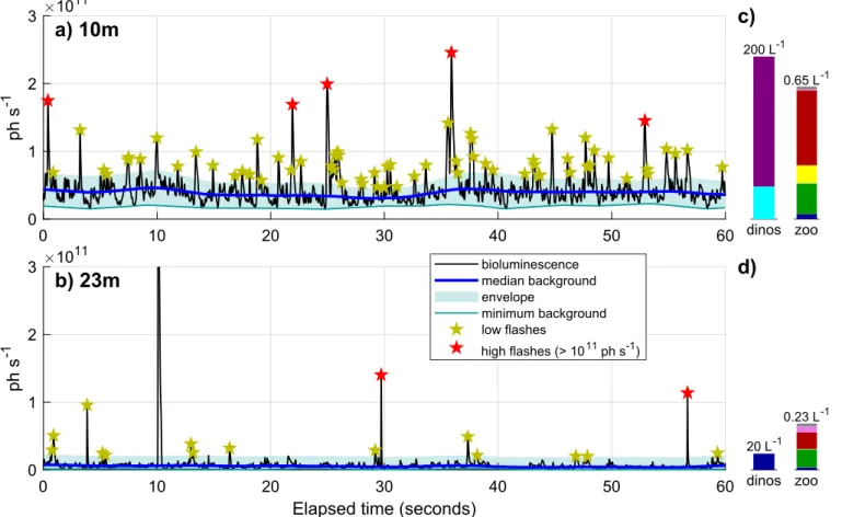
Background and flashes are estimated in a 3-step process detailed in Appendix B(Fig. 2d and3). Briefly, the background representing the mean dinoflagellate bioluminescence is first calculated using a median sliding window method (med_bg, blue line). Second, an envelope is defined to capture the range of variation of the dinoflagellate signal (teal shading): the bottom limit (min_bg, teal line) is obtained using a minimum sliding window method, and the upper limit defined by symmetry around med_bg (see Appendix B). The assumption is that flashes within the envelope are generated by dinoflagellates while fla-shes above are generated by zooplankton. Third, flafla-shes above the envelope are identified (stars) and their intensity defined relative to
med_bg. To avoid very dim flashes when min_bg is low (e.g.,Fig. 3b), a minimum envelope value of 1.5 × 10¹⁰ph s−1was set, corresponding
to an approximate lower limit for zooplankton flash intensity. Flashes are further categorized into “low” and “high” intensity (yellow and red stars, respectively), as separated by a 1011ph s−1 threshold (see
Appendix BandFig. B2).
Dinoflagellate and zooplankton proxies are defined as follows. The dinoflagellate proxy is min_bg divided by the flow rate (see Eq.(1)), termed bg_BL. Min_bg rather than med_bg was chosen because med_bg is more sensitive to zooplankton when their concentration is high (further discussed inSection 4.1). We consider that bg_BL is a proxy for all
Table 1
Acronyms for mathematical variables.
B Bioluminescence (measured) ph s−1
F Flow rate L s−1
BL Bioluminescence expressed per liter (= B / F) ph L−1 [BLS] Bioluminescent source concentration (equal to
concentration if each organism flashes once within the chamber)
L−1
TMSL Total Mechanically Stimulable Light ph individual−1 min_bg Minimum bioluminescence background ph s−1 med_bg Median bioluminescence background ph s−1 bg_BL Minimum bioluminescence background
expressed per liter (= min_bg / F) ph L
−1
fluo Fluorescence raw units
ratioAdinos bg_BL / fluo ratio for a given population of
dinoflagellates as well as bioluminescent dinoflagellates, because both are highly correlated (r = 0.52, p < 0.01 for the dataset displayed in Fig. 1; r > 0.8 for SPOKES-2002 and AOSN-2003 when considered separately). Zooplankton proxies are based on flashes: the number of flashes per liter is used as a proxy for larvaceans (low intensity flashes) and copepods (high intensity flashes) while the maximum flash in-tensity is used as a proxy for small jellies. The rationale is that (1) larvacean flashes are dimmer than other types of zooplankton including copepods, (2) larvacean and copepods are common enough where a flash intensity threshold can be determined from sensitivity analysis (seeAppendix B), and (3) while jellies are brightest and could theore-tically be determined using another flash intensity threshold, they are too rare for this threshold to be determined but their presence should be indicated by very bright flashes.
Proxy calculations were applied to the simulated time series (blue/ teal lines and yellow stars in Fig. 2d) to assess how successful the
method is in separating the dinoflagellate and zooplankton signals. The resulting proxies do capture the correct dinoflagellate bioluminescence (med_bg = 4.2 × 10¹⁰ph s−1, to be compared with the prescribed mean
dinoflagellate bioluminescence of 3.9 × 10¹⁰ph s−1) and zooplankton
flash concentration (2.25 flashes L−1compared to the prescribed
zoo-plankton concentration of 2.13 L−1). Most of the simulated zooplankton
flashes (Fig. 2b) were picked up by the proxy processing (Fig. 2d, yellow stars). A few were not (merging flashes counted as one) and some fla-shes were identified that belonged to the dinoflagellate rather than zooplankton time series (e.g., first yellow star), but overall the proxies succeeded in separating the simulated dinoflagellate and zooplankton signals.
2.4. Dinoflagellates and other phytoplankton
Fluorescence (fluo) is used in conjunction with the dinoflagellate
Table 2
Published flash kinetics for species commonly observed in Monterey Bay, either measured or reported as “most probable value” (averaged when several species were reported in the same paper, excluding larval stages). This table supports the concept that zooplankton bioluminescence is higher than for dinoflagellates, noting that studies may not be directly intercomparable as they represent different regions, species and organism physiological status. Studies that include both zooplankton and dinoflagellates species support zooplankton having higher flash intensity (21) and TMSL (10, 14) than dinoflagellates. See text andAppendix Aregarding the last two entries,*indicates numbers inferred fromFig. 3a. Gonyaulax polyedra is now placed in the genus Lingulodinium, and Gonyaulax catenella / acatenella / tamarensis are
now placed in the genus Alexandrium. Flash duration is typically defined for B > 3% of flash intensity (15) and was approximated for (20) and (21) as 2 × Tmax (time until the emission reached maximum). The relationship between TMSL (Total Mechanically Stimulable Light; ph cell−1) and quantum emission (/flash, ph flash −1) depends on the number of flashes per cell, ∼2–3 for Ceratium and Lingulodinium (see (16)). References:(1) Esaias et al. (1973), (2)Morin (1983), (3)Galt and
Sykes (1983), (4)Lapota and Losee (1984); (5)Galt et al. (1985), (6)Galt and Grober (1985), (7)Herring (1988), (8)Lapota et al. (1989), (9)Batchelder and Swift (1989), (10)Buskey and Swift (1990), (11)Batchelder et al. (1992), (12)Buskey (1992), (13)Herring et al. (1993), (14)Swift et al. (1995), (15)Latz and Jeong (1996, their Tables 4 & 5), (16)Latz et al. (2004), (17)Lapota (2012b), (18)Craig and Priede (2012), (19)Valiadi and Iglesias-Rodriguez (2013), (20)Johnsen et al. (2014), (21)Cronin et al. (2016).
Genus (% biolum species from (19)) TMSL (ph cell−1, ph flash−1) flash intensity (ph s−1) flash duration(ms)
Autotrophic dinoflagellates Ceratium (5%) ∼3 × 10⁸(1)
5.3 × 10⁸(10) 5.4 × 10⁸(11) 3 × 10⁸(14) 4.8 × 10⁸(17) (/flash) 108(4) (/flash) 9.7 × 10⁷(8) (/flash) 1.1 × 10⁸(18) 3 × 10⁸(4) 1.1 × 10⁹(16) 180–270 (4)239 (16) 200 (18) Alexandrium (23%) ∼5 × 10⁷(1) 107(19) Lingulodinium (50%) 2.4 × 10⁸(17) (/flash) 1.9 × 10⁸(18) 1.9 × 10 8(16) 100–150 (16) 100 (18) 130–150 (19) Heterotrophic dinoflagellates Protoperidinium (11%) 2.1 × 10⁹(10)
2 × 10⁹(11) 109(13) 1.9 × 10⁹(14) 2.8 × 10⁹(17) (/flash) 2.5 × 10⁹(8) 2.6 × 10⁹(15) 109(21) 135 (15)∼160 (21) Larvacean Oikopleura 3 × 10¹¹(9) 9.3 × 10¹⁰(10) 5 × 10¹¹(13, 5) 1011(11) 5.6 × 10¹¹(12) 109(2) up to 1.5 × 10¹²(6) 138 (2)278 (3) ∼150 (5) Copepod Metridia 9.5 × 10¹⁰(14) 7.1 × 10¹⁰(9) 1.4 × 10¹²(12) (/flash) 3.44 × 10¹²(18) (/flash) 1.2 × 10¹¹(8) 6.4 × 10¹²(7) 2.1 × 10⁹(20) 6.5 × 10⁹(21) 6700 (18) ∼400 (20) ∼260 (21) Oncaea 4.2 × 10⁹(13) 6.7 × 10⁸(13) ∼130 (13) Euphausiid Thysanoessa 2 × 10¹¹(9) 9.4 × 10¹⁰(10) 4 × 10⁹(12) 1.1 × 10¹¹(14) (/flash) 4 × 10⁹(8) 2.5 × 10¹⁰(21) ∼440 (21) Nyctiphanes (/flash) ∼ 1011(4) 1.75 × 10¹⁰(4) ∼3000–7000 (4) Ctenophore Beroe 1011(20) 2 × 10¹¹(21) 100–1600 (2)∼2200 (20) ∼1400 (21) Modeled dinoflagellates 6 × 108 * 5.4 × 109 250 Modeled zooplankton 1010 4.4 × 1010 * 500
proxy bg_BL to refine the dinoflagellate proxy into autotrophic (high fluorescence) and heterotrophic (low fluorescence) populations (Fig. 4a). When bioluminescence is low and fluorescence high, non-di-noflagellate phytoplankton dominate. These can include diatoms, fla-gellates, prymnesiophytes, picoplankton, etc. In coastal regions such as Monterey Bay, diatoms and dinoflagellates dominate the phytoplankton population and fluorescence signal (Chavez et al., 2017). Cases where fluorescence is high and bioluminescence low are thus attributed to diatoms in this paper, noting that other types of plankton can con-tribute to this signal particularly in other regions. While several dino-flagellate species are non-bioluminescent, bioluminescent and total dinoflagellate concentrations are highly correlated as explained above. By contrast, diatoms and dinoflagellates succeed each other, and are favored by different environmental conditions and less likely to coha-bitate (Margalef, 1978; Smayda and Trainer, 2010).
Proxies for heterotrophic dinoflagellates (h-dinos), autotrophic dinoflagellates (a-dinos), and other phytoplankton (a-other, mostly diatoms in our datasets) are computed for a given fluorescence/ bioluminescence dataset by assuming that the autotrophic dino-flagellate population (bioluminescent or not) is characterized by a constant bg_BL / fluo ratio, termed ratioAdinos. Details and equations are provided inAppendix B. Briefly, ratioAdinos is estimated from histograms as the most frequently observed bg_BL / fluo ratio. The
a-dino, h-dino and a-other proxies are defined based on their location in
the bg_BL, fluo space relative to ratioAdinos (Fig. 4b). These proxies, expressed in fluorescence units, are then normalized to the fluores-cence 99th percentile value. “Dominance” of one plankton type is based on the highest proxy and can be understood as follows: a-dinos dominate when their fluorescence is higher than a-other fluorescence and their bioluminescence higher than h-dino bioluminescence;
a-other dominate when their fluorescence is higher than a-dino
fluor-escence; and h-dinos dominate when their bioluminescence is higher than a-dino bioluminescence.
2.5. Application to field campaigns
Fluorescence and bioluminescence datasets, as well as in situ plankton counts, were collected during three field campaigns. These took place in Monterey Bay, California in Aug 24-Sep 2, 2000 (MUSE-2000), Aug 21–26, 2002 (SPOKES-2002), and Aug 10–16, 2003 (AOSN-2003). The objective of these field campaigns was to use a variety of platforms to obtain bay-wide distributions of biooptical parameters, along with corresponding plankton distributions, so they could be mapped to oceanographic features. As part of these efforts, fluorescence and bioluminescence sensors were deployed onboard ships, towfish and AUVs. Ship-based water samples for phytoplankton and zooplankton were collected using a CTD-rosette for phytoplankton and a 160 L Schindler trap for zooplankton (Fig. 1). Both methods allow for discrete sampling of a known volume of seawater from a well-constrained depth. Sampling varied across campaigns and days, following AUV surveys laid out in order to transition from nearshore to offshore en-vironments. Sample depths ranged from the surface to ∼40 m targeting zones above, at, and below the predominant thermocline, which was often associated with a band of high fluorescence. Samples were en-umerated by microscopic examination. Both dinoflagellates and zoo-plankton (bioluminescent or not) were fully enumerated; orders of magnitude were estimated for diatoms and converted into approximate numerical values.
This paper focuses on two autonomous datasets and matching in situ counts: (1) bioluminescence measured by a BP attached to a shipboard Schindler trap (all campaigns), and (2) fluorescence and biolumines-cence measured by a Dorado-class AUV (AOSN-2003). The first dataset is used to validate the bioluminescence proxies using plankton counts from all field campaigns (Section 3.1), and the second dataset is used for h-dino/a-dino/a-other proxy calculation (Section 3.2) and further analysis of the entire set of proxies (Section 3.3). Even though valida-tions of the AUV proxies using shipboard samples is complicated by space and time lags, the AUV dataset was chosen because the
h-dino/a-Fig. 2. Example of simulated bioluminescence time series. Flash kinetics (a) were chosen as typical of dinoflagellates (low intensity, short duration) and zooplankton
(high intensity, longer duration) followingTable 2and calculations based on Eq.(1)(seeAppendix A). The concentrations of bioluminescent sources ([BLS]) correspond to dinoflagellate and zooplankton concentrations inFig. 3a; the zooplankton number was increased by considering that each larvacean corresponds to 5
BLS (luminescent inclusions in the house,Galt and Grober, 1985). The time series are separately constructed for zooplankton (b) and dinoflagellates (c) by calculating the average temporal interval between flashes based on concentration and a given flow rate (326 mL s−1as inFig. 3a), randomizing the time steps when flashes peak,
and summing the individual flashes. The sum of the dinoflagellates and zooplankton time series (d, black) qualitatively and quantitatively captures the type of variability measured by the BP (Fig. 3a, seeTable 3). Blue/teal lines and yellow stars are proxies computed on the simulated time series (Section 2.3). (For interpretation of the references to colour in this figure legend, the reader is referred to the web version of this article.)
dino/a-other proxies require both fluorescence and bioluminescence to
be simultaneously measured. This rules out shipboard datasets because the CTD (fluorescence) and Schindler trap (bioluminescence) were se-quentially deployed.
Different generations of MBBPs were used across campaigns, the
main difference being the temporal resolution: 60 Hz for AOSN-2003, 1 Hz for MUSE-2000 and SPOKES-2002 (see Appendix B). This is a significant difference as typical flash durations can be 100–200 ms (Table 2), thus flashes are fully resolved with the 17 ms time step of the 60 Hz sensor but not with the 1 s time step of the 1 Hz sensors. The proxy method was directly applied to AOSN-2003 but had to be adapted for MUSE-2000 and SPOKES-2002. The min_bg bioluminescence was estimated using a similar sliding window technique. “Flashes” were identified as peaks in the 1 Hz signal above min_bg plus a given threshold specific to each field campaign (details inAppendix B). These thresholds, as well as other proxy parameters such as the sliding window used to define the background, were optimized through sen-sitivity tests based on correlations with in situ counts, where a range of values is attributed to a parameter while holding the others constant. The parameter resulting in the highest correlation with in situ counts was chosen (SeeAppendix BandFig. B2).
3. Results
3.1. Comparison of bioluminescence proxies to in situ counts
The bioluminescent plankton communities during the three cam-paigns were diverse although they shared some characteristics (Fig. 1). Bioluminescent dinoflagellate concentration was higher near the sur-face; the main genera included Protoperidinium, Alexandrium, Ceratium and Lingulodinium. These genera include luminous and non-luminous species (Valiadi and Iglesias-Rodriguez, 2013), and we did not de-termine whether the sampled species were bioluminescent.
Fig. 3. Example of 60 Hz bioluminescence time series measured on Aug 15, 2003 (AOSN-2003 field campaign). The black line represents one minute of
biolumi-nescence measured for a surface (a, 10 m) and subsurface (b, 23 m) sample at the same station. The proxies are indicated by blue/teal lines (dinoflagellate back-ground bioluminescence) and stars (zooplankton flashes); blue shading highlights the bioluminescence envelope (dinoflagellate bioluminescence range of variation). The red star for the flash observed near 10 s in (b) is not visible because the flash peak (5.15 1011ph s−1) exceeds the range of the figure. The concentration and
composition of bioluminescent plankton based on matching in situ samples is given on the right (c and d, seeFig. 1for the color legend, y-axis are identical between 10 m and 23 m samples but different between dinoflagellates and zooplankton).
Table 3
Comparison of measured (Fig. 3a) and simulated (Fig. 2d) bioluminescence time series. Background bioluminescence, envelope and flashes are defined in
Section 2.3. Note that the simulated flash concentration is dictated by the measured zooplankton concentration (see text) and is less than the flash con-centration in the measured time series, which also has an impact on the var-iance.1A Hurst exponent close to 1 indicates a persistent time series (in the
short term, the direction of change is retained). This is related to autocorrela-tion and thus strongly dependent on the time resoluautocorrela-tion. Computed using
https://mathworks.com/matlabcentral/fileexchange/30076-generalized-hurst-exponent.
Measured time
series Simulated timeseries Mean (ph s−1) 4.5 × 10¹⁰ 4.6 × 10¹⁰
Variance (ph s−1) 2.4 × 10¹⁰ 1.6 × 10¹⁰
Autocorrelation at 50 ms (3 time steps) 0.85 0.89 Hurst exponent1(long-term memory of a
time-series) 0.71 0.80
Background bioluminescence med_bg (ph s−1) 3.9 × 10¹⁰ 4.2 × 10¹⁰
Ratio envelope/background
2 × (med_bg-min_bg)/med_bg 1.06 0.87
Flash concentration
Bioluminescent zooplankton was dominated by larvaceans followed by copepods; copepod concentration was higher in subsurface than surface samples. Bioluminescent zooplankton concentration was ∼2–3 orders of magnitude lower than dinoflagellates.
The bioluminescence proxies were computed from time series measured by the Schindler trap BP and correlated to matching in situ plankton concentration (Tables 4 and 5). Only correlations significant at the 5% level (p < 0.05) are reported. Statistical significance was
Fig. 4. Using fluorescence and bioluminescence to discriminate between non-dinoflagellate phytoplankton (mostly diatoms in Monterey Bay), autotrophic and
heterotrophic dinoflagellates. (a) Schematic illustrating the basic concept: fluorescence is high for autotrophic populations, while background bioluminescence is high for dinoflagellates. Plankton characterized by high fluorescence and low bioluminescence are mostly diatoms in coastal ecosystems, but can include other non-dinoflagellate phytoplankton particularly in other regions. (d) Mathematical definition of h-dino, a-dino and a-other proxies and associated dominance in the fluo,
bg_BL space (see equations inAppendix B). The slope of the black line is ratioAdinos (rA). The proxies are normalized such that a value of 1 corresponds to the 99th fluorescence percentile (fluo99). Labels for the dominance colorbar stand for h-dinos (HD), a-dinos (AD) and a-other (AO). (For interpretation of the references to colour in this figure legend, the reader is referred to the web version of this article.)
Table 4
Pearson correlation coefficients between bioluminescent plankton concentrations and 60 Hz bioluminescence proxies from the Schindler trap dataset (60 Hz is only available for AOSN 2003). “n.s.” indicates correlations non-significant at the 5% level,*correlations significant at the 1% level,**at the 0.1% level, bold expected
correlations. (*) correlation with samples collected at the BP exhaust: r = 0.81**(N = 18).
Background bioluminescence (ph L-1) Low intensity flashes (nb L-1) High intensity flashes (nb L-1) Maximum intensity (ph s-1)
Dinoflagellates (N=15) 0.60 n.s. n.s. n.s. Larvaceans (N=89) 0.48** 0.46** n.s. n.s. Larvaceans < 3.5 L-1(N=83) 0.43** 0.55** n.s. n.s. Copepods (N=89) n.s. n.s. 0.33*(*) n.s. Small jellies (N=89) n.s. n.s. n.s. 0.31* Table 5
Pearson correlation coefficients between bioluminescent plankton concentrations and 1 Hz bioluminescence proxies from the Schindler trap dataset. “n.s.” indicates correlations non-significant at the 5% level,*correlations significant at the 1% level,**at the 0.1% level, bold expected correlations (dinoflagellates with bg_BL,
zooplankton with flashes). Numbers of samples are given for each campaign. The AOSN-2003 bioluminescence was adjusted using a 2.63 factor in the “combined” correlations to account for a change in BP (seeAppendix B).
Background bioluminescence (ph L-1) Flash concentration (nb L-1)
Dinoflagellates 0.44** n.s. MUSE-2000 (N=84) 0.65** n.s. SPOKES-2002 (N=29) 0.52 n.s. AOSN-2003 (N=15) — — — 0.49** 0.23* combined (N=128) Zooplankton 0.36** 0.34** MUSE-2000 (N=96) 0.38 0.49* SPOKES-2002 (N=39) 0.39** 0.45** AOSN-2003 (N=89) — — — 0.18* 0.29** combined (N=224)
estimated by assuming all samples are independent, which is a rea-sonable assumption for patchy biological populations. As an example, during AOSN-2003 samples were separated by ∼3–4 km and > 1 h horizontally, 4–5 m and ∼15 min vertically (for the closest depths). Simple calculations based on current velocities (∼0.2–0.4 m/s hor-izontal and 10−4to 10−3m/s vertical,Shulman et al., 2015) and
di-noflagellate vertical migration speeds (< 40 m day-1,Shulman et al., 2012) indicate that sampling occurred faster than plankton populations
could travel. A possible exception are copepods, for which swimming speeds (∼3–5 mm/s for Metridia pacifica,Wong, 1988) could approach vertical sampling speed for the closest stations; however, copepods are extremely patchy and mostly found deeper where vertical separation between samples increases. Repeat sections were rare and separated by several days.
Proxies computed for the AOSN-2003 field campaign (60 Hz data available) were able to separate between larvaceans, copepods and
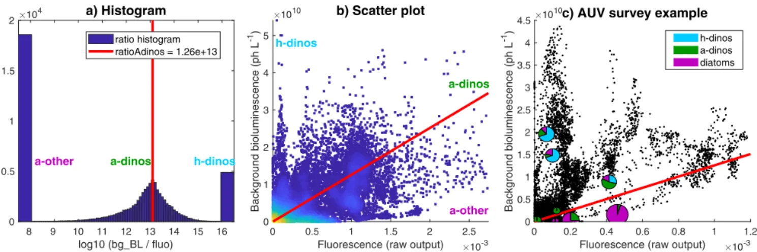
Fig. 5. Determination of ratioAdinos (ratio of background bioluminescence to fluorescence for autotrophic dinoflagellates) for the AOSN-2003 Dorado dataset. (a)
Histogram of all measured nighttime bg_BL/fluo ratios during the campaign. The x-axis was set to highlight the most common ratio (ratioAdinos, red line); the left and right bars correspond to values less or equal to 8 and higher or equal to 16, respectively. (b) Scatter plot of bg_BL versus fluorescence during AOSN-2003 (colors indicate the density of data points). The red line highlights ratioAdinos. (c) Example of plankton composition as a function of matching AUV fluorescence and background bioluminescence averaged within a 30 s window around each sample location. Black dots represent the fluo, bg_BL dataset for the August 15–16, 2003 nighttime AUV survey. Pie charts are plankton samples taken along the AUV track and located in fluo, bg_BL space according to AUV measurement at the same location. Colors represent the plankton composition; the size is proportional to plankton concentration (dinoflagellates include both bioluminescent and non-bioluminescent species). The red line highlights ratioAdinos (note that axes are different between b and c). (For interpretation of the references to colour in this figure legend, the reader is referred to the web version of this article.)
Fig. 6. Two examples of Dorado profiles on the August 15–16, 2003 nighttime survey (identified by blue triangles inFig. 7) and associated proxies. Fluorescence and background bioluminescence (panels a & c) are used to calculate proxies for h-dinos, a-dinos and a-other (b & d) based on the relationships displayed inFig. 4. The axes for fluo and bg_BL are set such that their ratio is equal to ratioAdinos when they superimpose; areas shaded in pink, green and blue in (a) and (c) thus correspond to
h-dinos, a-dinos and a-other in (b) and (d) as indicated by the color arrows. More precisely, the lower of the fluo (red) and bg_BL (teal) lines is attributed to a-dinos
(green); the difference between the fluo and bg_BL lines is attributed to a-other (purple) when fluo is higher (as in profile 2), and to h-dinos (soft blue) when fluo is lower (as in profile 1). (For interpretation of the references to colour in this figure legend, the reader is referred to the web version of this article.)
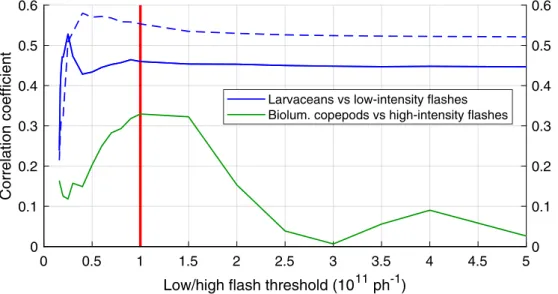
small jellies as each zooplankton proxy was only significantly corre-lated with its target (bold numbers inTable 4). Background biolumi-nescence was correlated with both dinoflagellates and larvaceans, but more strongly with dinoflagellates. In general, correlations were higher for dinoflagellates (r = 0.60) than for zooplankton (r = 0.31–0.46); correlations for copepods and small jellies were significant at the 1% level but low (0.31–0.33). These zooplankton are rare and extremely patchy, and likely to exhibit avoidance behaviors, which may explain the low correlations. This is supported by the much higher correlation found for copepods when considering samples directly collected at the BP exhaust (r = 0.81, N = 18). Interestingly, correlations between larvaceans and low-intensity flashes, while relatively high (r = 0.46), were unexpectedly lower than correlations with bg_BL (r = 0.48). This is likely due to (1) larvaceans being highly correlated with dino-flagellates (r = 0.76, N = 14) and low-intensity flashes being correlated with bg_BL (r = 0.56, N = 89), and (2) larvaceans contributing to background bioluminescence when their concentration is high (dis-cussed inSection 4.1). Indeed, excluding the few samples with larva-cean concentrations greater than 3.5 L−1increased the larvacean
cor-relation with flashes to 0.55 and decreased the corcor-relation with bg_BL to 0.43 (Table 4).
Only 1 Hz data was available for the other two campaigns, which
does not allow flash resolution. The performance of proxies adapted for 1 Hz time series was assessed by computing both 1 Hz and 60 Hz proxies for AOSN-2003. Across the entire AUV nighttime dataset, their corre-lation is very high for bg_BL (r = 0.95) and lower for flashes (r = 0.76 for flashes per liter averaged over 15 sec windows), suggesting that 1 Hz is sufficient to resolve dinoflagellates but less so zooplankton. Consistent with this assessment, for AOSN-2003 the correlation be-tween bg_BL and dinoflagellates only slightly decreased by using 1 Hz data (0.52 instead of 0.60, Tables 4 and 5). Even without flash re-solution, 1 Hz bioluminescence proxies significantly correlated with the dinoflagellate and zooplankton concentrations during all three cam-paigns (Table 5). Correlations between 1 Hz bg_BL and dinoflagellate concentrations range from 0.44 to 0.65, and reach 0.49 when con-sidering all three campaigns together. Correlations between zoo-plankton concentrations and the 1 Hz flash proxy ranged from 0.34 to 0.49, decreasing to 0.29 for the combined dataset. These low correla-tions are not surprising since 1 Hz time series do not resolve individual flashes. With the exception of zooplankton for MUSE-2000, zoo-plankton correlations with flashes are stronger than with bg_BL, and dinoflagellate correlations with bg_BL are always stronger than with flashes.
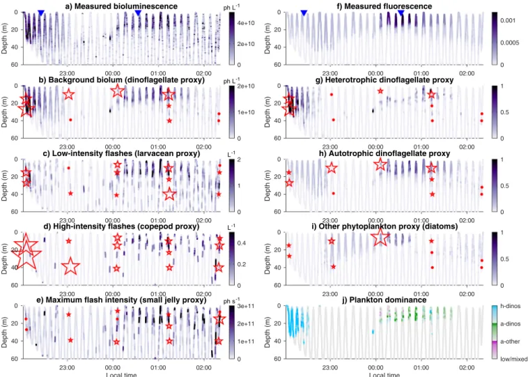
Fig. 7. Bioluminescence and fluorescence Dorado sections on the night of August 15–16, 2003 (top) and derived proxies (bioluminescence proxies on the left,
fluorescence/bioluminescence on the right). The red stars/dots represent shipboard in situ counts along the same section (taken within 600 m of each location and 2 h of AUV sampling), including both bioluminescent and non-bioluminescent species. The stars are counts scaled for each variable, dots indicate where the count was 0. The scaling factor is identical for a-dinos and h-dinos, but different for diatoms, which were only qualitatively estimated. Plankton dominance in (j) is attributed to whichever has the highest proxy, and the value for the color mapping is the difference between the dominant and the next highest proxy (colorbars range: 0–0.4). When the value of the dominant proxy is < 0.2, dominance is set to 0 (low/mixed). Blue triangles in the top panels identify the two vertical profiles displayed in
Fig. 6. The two high-copepod samples at the beginning contained no bioluminescent species. (For interpretation of the references to colour in this figure legend, the reader is referred to the web version of this article.)
3.2. Fluorescence / bioluminescence proxies during the AOSN-2003 field campaign
H-dino, a-dino and a-other proxies were computed from the AUV
Dorado nighttime dataset collected during the AOSN-2003 field cam-paign (August 10–16, 2003). For this dataset, fluorescence and biolu-minescence are decoupled (r = 0.38). Fluorescence and background bioluminescence, while more strongly correlated, share less than half of their variance (r = 0.65) suggesting that the plankton community al-ternated between h-dinos, a-dinos and a-other (diatoms). The only parameter needed to define the proxies, ratioAdinos, was determined from the Dorado dataset by analyzing the ratio of the 60 Hz background bioluminescence and fluorescence, both regridded at a 1 Hz resolution. A histogram of the ratio clearly separates low (a-other), high (h-dinos) and intermediate (a-dinos) ratios (Fig. 5a). These intermediate ratios were most frequently around 1.26 × 10¹³, chosen as ratioAdinos (unit
undefined since fluorescence was raw data). Each point in the fluo,
bg_BL space can be attributed to h-dinos, a-dinos or a-other populations
based on its position relative to the ratioAdinos line (Fig. 4); in situ counts support this concept (Fig. 5c). The proxies were computed in fluorescence units and normalized to the fluorescence 99th percentile. As an example,Fig. 6displays two contrasting AUV profiles and their corresponding proxies. The first profile (Fig. 6a and b) is char-acterized by much higher bg_BL than fluo (with the ratioAdinos con-version), indicative of a community dominated by heterotrophic dino-flagellates as represented by the high h-dino proxy. The second profile (Fig. 6c and d) displays higher fluo than bg_BL in the top 15 m (with the
ratioAdinos conversion), hence h-dino = 0 and a-other > 0. While
lower, bg_BL remained relatively high. This suggests that autotrophic dinoflagellates were also present and that the phytoplankton commu-nity near profile 2 was a mix of diatoms and dinoflagellates (Fig. 6d). This was confirmed by samples taken nearby (Fig. 7, near midnight).
Correlations between AUV-based proxies and shipboard plankton counts are not straightforward because of time and space lags; more-over, only orders of magnitude were estimated for diatoms. Diatom
(a-other) and dinoflagellate proxies were qualitatively compared with
available plankton counts; an example is displayed inFig. 7for the last survey (August 15–16). The AUV track started near the Año Nuevo upwelling center and ended at an offshore location near 122.3°W, 36.8°N (seeFig. 8). This specific survey was chosen because 10 of the 15 AOSN-2003 phytoplankton samples correspond to this section.Fig. 7 illustrates how, from only two measured parameters (bioluminescence and fluorescence), a suite of proxies can be derived characterizing the phyto- and zooplankton communities. The proxies indicate that the community was dominated by heterotrophic dinoflagellates nearshore around 20 m (Fig. 7g, j), a mix of diatoms and autotrophic dino-flagellates in the middle of the transect and closer to the surface (Fig. 7h–j), larvaceans in similar locations as dinoflagellates but also deeper (Fig. 7c), and copepods and small jellies in patchy locations offshore, mostly in the top 30 m (Fig. 7d, e). In situ counts along the transect (red stars/dots) support these results, particularly for the diatom and dinoflagellate communities (right column). While zoo-plankton patterns are generally similar between proxies and in situ counts, the agreement is not as good as for diatoms and dinoflagellates. This was expected because of the patchiness of zooplankton populations and time/space lags (samples were taken within 600 m of the AUV track but on average an hour later). Relationships improve slightly when comparing the proxies to counts of bioluminescent species only, parti-cularly for copepods at the beginning of the section (the 2 samples near 10 pm only had non-bioluminescent copepod species).
3.3. Analysis of the AOSN-2003 Dorado dataset
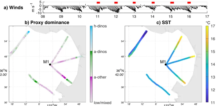
Combining all the Dorado surveys provides a picture of plankton communities in Monterey Bay during upwelling conditions and high-lights the potential of the method (Fig. 8). A single map was built be-cause winds were consistently upwelling-favorable (Shulman et al., 2011; Fig. 8a), suggesting that spatial variability was likely stronger than temporal variability. The proxies indicate that dinoflagellates dominated near shore while other phytoplankton (here diatoms) were
Fig. 8. Dorado nighttime surveys during the AOSN-2003 field campaign (Aug. 11–16). (a) Wind vectors measured at station M1, with Dorado surveys highlighted by
red bars. Winds were upwelling-favorable the whole time. (b) Average proxies in the top 50 m were used to calculate plankton dominance by heterotrophic dinoflagellates (blue), autotrophic dinoflagellates (green) and other phytoplankton (diatoms, purple) following the same logic asFig. 7j. Here the color bar range is 0–0.3. (c) Sea surface temperature defined as the point closest to the surface for each profile (generally in the top 2 m). The section displayed inFig. 7is located off Año Nuevo (north-westernmost track). (For interpretation of the references to colour in this figure legend, the reader is referred to the web version of this article.)
more abundant inside the bay (Fig. 8b). This plankton distribution mirrors the surface temperature measured by the vehicle (Fig. 8c) with dinoflagellates dominating in warm waters and diatoms in colder wa-ters. This is consistent with the model presented bySmayda and Trainer (2010)in which diatoms bloom first when upwelling intensifies, then dinoflagellates bloom when upwelling relaxes. Spatially, this translates into diatoms dominating recently (cold) upwelled waters and dino-flagellates dominating older (warmer) waters as illustrated byFig. 8. Dinoflagellate vertical migration could also contribute to the inshore/ offshore difference in plankton composition, as dinoflagellates from the northern bay were able to avoid advection by the strong southward surface currents by migrating deeper, while non-migrating diatoms were advected (Shulman et al., 2011, 2012).
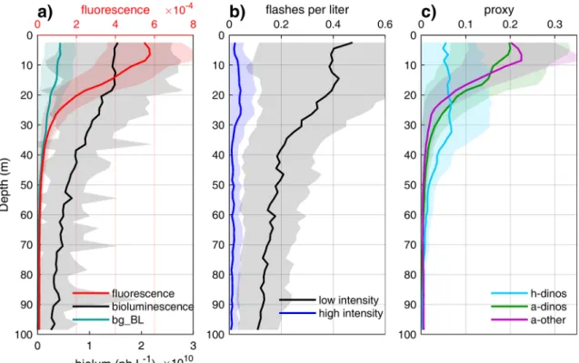
Average fluorescence, bioluminescence and proxy profiles provide additional information regarding the vertical distribution of different plankton types during AOSN-2003 (Fig. 9). Fluorescence peaked in the top 10 m and sharply decreased with depth, while bioluminescence was highest down to 20 m and slowly decreased through the water column (Fig. 9a). Bioluminescent flashes (zooplankton) remained numerous down to 100 m where their density was still ∼25% of the surface density (Fig. 9b); copepods (high-intensity flashes) peaked deeper than larvaceans (low-intensity flashes). Flashes were responsible for the very high variability in the bioluminescence time series relative to fluores-cence, as illustrated by the standard deviation in relation to the mean. By contrast, bg_BL (dinoflagellate proxy) was considerably less variable and slowly decreased with depth, becoming negligible below 50 m. The
h-dino, a-dino and a-other proxies (Fig. 9c) suggest that heterotrophic dinoflagellates tend to occur deeper in the water column than phyto-plankton (a-dinos + a-other). Phytophyto-plankton vertical distribution was similar between autotrophic dinoflagellates and other phytoplankton (diatoms), although dinoflagellates remained high slightly deeper than diatoms.
4. Discussion
4.1. Validating the method: Insights from simulated time series
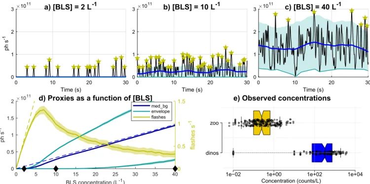
The proxies rely on the assumption that dinoflagellates’ numerous low-intensity flashes merge to generate a bioluminescent background, whereas zooplankton emit infrequent high-intensity flashes above the background. Here we revisit this assumption using the simulated time series presented in Section 2.2 (Fig. 10). Time series were generated for varying con-centrations of bioluminescent sources ([BLS]) and for a given plankton type characterized by its flash kinetics, here chosen to represent zoo-plankton (Fig. 2a). The goal was to analyze how the bioluminescence signal changes as a function of concentration for a given species, and to verify whether the proxies indeed correlate with plankton concentrations. For very low concentrations ([BLS] < ∼4 L−1, e.g.,Fig. 10a), the
number of flashes (yellow) is proportional to [BLS] for simulated time series, following the theoretical dashed yellow line. In this case both
min_bg (teal) and med_bg (dark blue) are close to 0. For higher
con-centrations ([BLS] > ∼4 L−1), the flash density becomes high enough
where flashes start to merge (med_bg > 0,Fig. 10b). The flash proxy still increases with [BLS] until ∼6–7 L−1 but becomes lower than
theoretical values, and above ∼6–7 L−1becomes unreliable as it
de-creases with increasing [BLS] (Fig. 10d). Regarding the background, once flashes begin to merge and a background is generated (i.e. for [BLS] > 4 L−1), med_bg increases with [BLS] and tracks the theoretical
background computed from Eq.(1)(dashed blue line inFig. 10d). By contrast, min_bg only becomes positive for [BLS] > ∼20 L−1 (e.g.,
Fig. 10c) then also increases with [BLS] following med_bg. In the si-mulations, these thresholds are sensitive to the flash duration (here 500 ms) but not to flash intensity. For shorter flash duration thresholds are higher (∼10 L−1 and 60 L−1 for a typical dinoflagellate flash
duration of 200 ms instead of ∼4 L−1 and 20 L−1, not shown). To
summarize, this exercise illustrates how [BLS] is correlated to flashes at low concentrations ([BLS] < ∼6–7 L−1 for zooplankton), to med_bg
Fig. 9. Average vertical profiles for fluorescence, bioluminescence and derived proxies during the AOSN-2003 field campaign. The profiles were computed in 2 m
bins, each averaging ∼ 1500 data points except near the surface and 100 m where the AUV turns, sharply increasing the number of data points to > 5000. In (a),
bg_BL is computed from min_bg (proportional to dinoflagellates but not representing dinoflagellate bioluminescence). The width of the shading represents the standard
except at very low concentrations (< ∼4 L−1), and to min_bg when
concentrations are high enough ([BLS] > 20 L−1 for zooplankton,
60 L−1for dinoflagellates) (Fig. 10d).
Fig. 10d can be used to assess the validity of the proxies based on observed concentrations (Fig. 10e). Zooplankton concentrations mea-sured during the 3 field campaigns were ∼0.25 L−1and mostly below
2 L−1. Zooplankton may flash several times and larvacean houses
contain several bioluminescent inclusions, which could increase [BLS] to ∼1–2 L−1and mostly below 10 L−1. For these concentrations, the
flash proxy is proportional to [BLS] although it would underestimate zooplankton for high concentrations (> 4 L−1). AOSN-2003
correla-tions supports this hypothesis by showing a increase in performance for the larvacean proxy when excluding samples with larvacean con-centrations > 3.5 L−1, also corresponding to bioluminescent
zoo-plankton > 4 L−1(“high BLzoo samples”, 7% of the samples,Table 4).
The validity of the dinoflagellate proxy can also be estimated from Fig. 10d as a function of concentration. Measured bioluminescent di-noflagellate concentrations were most often > 100 L−1, a situation
where both min_bg and med_bg are proportional to [BLS] (Fig. 10d, noting that in dinoflagellate simulations with shorter duration flashes,
min_bg becomes > 0 above ∼ 60 L−1 instead of ∼ 20 L−1). Either
min_bg or med_bg can be used as a dinoflagellate proxy since both are
highly correlated (r = 0.96 in the AOSN-2003 AUV dataset). However,
med_bg is sensitive to zooplankton above ∼4 L−1while min_bg only
becomes > 0 at much higher zooplankton concentrations (∼20 L−1).
Min_bg is thus a better dinoflagellate proxy as it is less likely to be
“contaminated” by zooplankton.
A previous paper introduced the time series coefficient of variation (CV, standard deviation divided by mean) as a tool to separate between dinoflagellates and zooplankton (Moline et al., 2009). The simulated time series were used to assess how CV varies as a function of [BLS], similar to
the results presented inFig. 10. For a given plankton type characterized by its flash kinetics, CV decreases exponentially with [BLS] such that 1/CV is strongly correlated with [BLS] and the mean bioluminescence (r = 0.99 for simulations shown inFig. 10). This is directly due to flashes merging when concentration increases, decreasing CV (visible in Fig. 10a–c for which CV = 2.3, 0.9 and 0.4, respectively). No correlations were found between CV and in situ plankton concentrations, also suggesting that CV is not an indicator of zooplankton or dinoflagellate concentration. However, when considering CV as a function of bioluminescence for dinoflagellates and zooplankton (from simulated time series with different flash kinetics), CV is indeed much higher for zooplankton than dinoflagellate populations (Fig. 11a). In the simulations, for typical concentrations CV was higher than 1 for zooplankton, lower than 1 for dinoflagellates, and about 3 times higher for zooplankton than dinoflagellates for a given bioluminescence value. These results justify the use of CV as a tool to separate between dinoflagellates and zooplankton as inMoline et al. (2009), noting that CV cannot be used as a proxy as it is inversely proportional to concentration. By contrast, the flash proxy presented here is also much higher for zoo-plankton than dinoflagellates, and is proportional to zoozoo-plankton con-centration except for very high concon-centrations (Fig. 10d and11b) so that it is a better zooplankton proxy.
4.2. Limitations of the plankton proxies
The results presented above support the use of bioluminescence- and fluorescence-derived variables as proxies for dinoflagellates, other phyto-plankton such as diatoms, and different types of zoophyto-plankton. The proxies were validated using simple correlations with in situ plankton counts (Tables 4 and 5). These correlations, while significant (p < 0.01 except for dinoflagellates during AOSN-2003 where p < 0.05), remain relatively low particularly for zooplankton (r < 0.5). This suggests that quantitative
Fig. 10. Investigating the effects of cell concentration on the shape of the bioluminescence signal and the validity of proxies. Top panels: examples of simulated 60 Hz
time series based on one plankton type (zooplankton) and increasing bioluminescence source concentrations ([BLS]). The corresponding proxies are displayed as blue lines and stars (seeFig. 2for the legend; low/high intensity flashes were not separated and the minimum envelope value of 1.5 × 10¹⁰ph−1was not applied). Bottom
panels: (d) evolution of proxies as a function of [BLS], obtained by averaging results from 100 simulations for each [BLS] (shading represents +/– 1 standard deviation around the mean, very small except for flashes). Black diamonds indicate the concentrations for which example time series are displayed in top panels. Dashed lines are theoretical relationships: [BLS] × F for flashes (yellow) and [BLS] × F × TMSL for background (blue) where F is the flow rate (cf Eq.(1)). (e) Observed plankton concentrations during the 3 field campaigns (log scale), plot generated using BoxPlotR (http://shiny.chemgrid.org/boxplotr/). Data points are plotted as open circles; center lines show the medians; box limits indicate the 25th and 75th percentiles as determined by R software; whiskers extend to 5th and 95th percentiles (the 95th percentile for zooplankton is ∼2 L−1); the width of the boxes is proportional to the square root of the sample size (N = 139 for dinos, 233 for
relationships are lacking at this point and that the zooplankton proxies should be considered with caution, particularly for small jellies and to a lesser extent copepods. Because each proxy is only correlated with its target population (Table 5), the proxies should at least provide qualitative evidence of changes in concentration for a given population.
There are several caveats associated with the method; perhaps the most important is that while the proxies capture changes in populations and the relative dominance of h-dinos/a-dinos/a-other (e.g.,Fig. 7), they cannot provide information on concentrations without proper calibra-tion based on in situ counts. Intercomparisons between different in-struments is difficult at best, as illustrated by the difference in biolu-minescence measured by two generations of BPs during the AOSN-2003 campaign (seeAppendix B). While in theory bioluminescence is a direct function of concentration, flow rate, and TMSL (Eq.(1)), in practice it also depends on pre-stimulation of organisms prior to reaching the BP chamber, and on the BP stimulation efficiency (Herren et al., 2005). Latz and Rohr (2013)systematically tested several BPs and found that these parameters vary with the BP design and the organisms tested, such that bioluminescence cannot be directly compared across instru-ments. In addition, which platform is used and how the BP is mounted can impact the signal as well, notably for zooplankton because of avoidance behavior. The bioluminescence proxies were primarily de-veloped based on data measured by a 60 Hz BP deployed during AOSN-2003 and later commercialized as the WET Labs UBAT (http://www. seabird.com/ubat). The method could thus be applied to other UBAT datasets, although parameters such as the minimum envelope and flash threshold would need to be adjusted. While the proxies could be adapted to different BP/fluorometer combinations, direct quantitative intercomparisons of resulting proxies would be difficult. Within the same dataset, the proxies are expected to be proportional to the con-centration of their target species, with a few caveats:
First, zooplankton proxies are only representative of the water being sampled by the BP, and may not be representative of local conditions because of organism patchiness and low concentrations. It is thus dif-ficult to relate a water sample to the signal measured by the BP even when taken close in space and time. This is particularly true for cope-pods and small jellies, for which significant but low (r = 0.31–0.33) correlations were found. This issue is illustrated by zooplankton sam-ples collected simultaneously from the Schindler trap and at the BP exhaust (N = 18). The correlation between the two sets of samples for copepod concentration was only 0.23, highlighting a strong small-scale
variability. The correlation between the number of high-intensity fla-shes and bioluminescent copepods increased from 0.24 for the Schindler trap samples to 0.81 for the BP exhaust samples.
Second, the larvacean proxy (low-intensity flashes) becomes unreliable both at high larvacean concentrations (Fig. 10d) and at high dinoflagellate concentrations (high background that would mask larvacean flashes). This is not an issue for the copepod proxy, as their concentrations are unlikely to exceed the threshold for flash proxy validity (∼6–7 L−1,Fig. 10d), and
their flashes are bright enough that only extreme dinoflagellate con-centrations would generate a background high enough to mask them. The larvacean proxy is also likely confounded by the fact that larvacean bio-luminescence originates from their house rather than from the animal it-self (Galt et al., 1985).Galt and Grober (1985)found that bioluminescence varies as a function of animal size and number of luminescent inclusions in the house, such that the number of flashes associated with each larvacean may vary widely.
Last, the separation of h-dinos, a-dinos and a-other relies on the as-sumption that bioluminescent and non-bioluminescent dinoflagellates co-vary such that the ratio of fluorescence to bioluminescence in a-dinos populations (ratioAdinos) remains constant. This assumption is supported by the correlation between bioluminescent and total dinoflagellate species in our dataset (r = 0.52, p < 0.01 over the three field campaigns).Kim et al. (2006)also reported a synchronous increase in both bioluminescent and non-bioluminescent dinoflagellate species during a bloom, and Marcinko et al. (2013b)identified a number of studies that found positive associations between bioluminescence and total dinoflagellate concentra-tion (bioluminescent or not). However, dinoflagellate communities can evolve over time, and ratioAdinos could for instance increase when the
a-dino population shifts towards more bioluminescent a-dinoflagellates
leading to an overestimate of h-dinos relative to a-other. Particularly in large datasets spanning very diverse communities, deviations from the average relationship are possible and would result in unreliable proxies.
5. Conclusions and perspectives
Using outputs from two autonomous sensors (fluorescence and biolu-minescence), a suite of proxies can be derived characterizing the coastal plankton community including non-dinoflagellate phytoplankton (e.g., diatoms), autotrophic dinoflagellates, heterotrophic dinoflagellates, lar-vaceans, copepods, and small jellies. Bathyphotometers thus bring tre-mendous added value relative to fluorometers alone, by extending
Fig. 11. Proxies as a function of bioluminescence for typical phytoplankton and zooplankton concentrations (from the simulated time series, unit flashes as in
Fig. 2a). For each phytoplankton and zooplankton concentration (colors), 100 1-min simulated time series were generated and the corresponding bioluminescence and proxies values averaged: (a) CV, (b) flashes, (c) min_bg. For a given bioluminescence value, simulated zooplankton populations (stars) exhibit a higher CV than simulated dinoflagellate population (triangles); however, CV is inversely proportional to concentration (a). The flash proxy is proportional to simulated zooplankton concentration except for high concentrations ([BLS] > 6 L−1, b) and min_bg is proportional to simulated dinoflagellate concentrations except for low concentrations