HAL Id: hal-01863541
https://hal.archives-ouvertes.fr/hal-01863541
Submitted on 1 Jun 2020
HAL is a multi-disciplinary open access
archive for the deposit and dissemination of
sci-entific research documents, whether they are
pub-lished or not. The documents may come from
teaching and research institutions in France or
abroad, or from public or private research centers.
L’archive ouverte pluridisciplinaire HAL, est
destinée au dépôt et à la diffusion de documents
scientifiques de niveau recherche, publiés ou non,
émanant des établissements d’enseignement et de
recherche français ou étrangers, des laboratoires
publics ou privés.
comparing SVAT models over wheat fields
A Olioso, Isabelle Braud, A Chanzy, D Courault, J Demarty, L Kergoat, E
Lewan, C Ottle, L Prevot, Wgg Zhao, et al.
To cite this version:
A Olioso, Isabelle Braud, A Chanzy, D Courault, J Demarty, et al.. SVAT modeling over the
Alpilles-ReSeDA experiment: comparing SVAT models over wheat fields. Agronomie, EDP Sciences, 2002, 22
(6), pp.651-668. �10.1051/agro:2002054�. �hal-01863541�
A. Olioso et al.
Comparing SVAT models over wheat fields
Original article
SVAT modeling over the Alpilles-ReSeDA experiment:
comparing SVAT models over wheat fields
Albert O
LIOSOa*, Isabelle B
RAUDb,c, André C
HANZYa, Dominique C
OURAULTa,
Jérôme D
EMARTYd,a, Laurent K
ERGOATi, Elisabet L
EWANf, Catherine O
TTLÉc,
Laurent P
RÉVOTa, Wenguang G. Z
HAOa, Jean-Christophe C
ALVETg, Pascale C
AYROLe,
Raymond J
ONGSCHAAPh, Sophie M
OULINe,a, Joël N
OILHANg, Jean-Pierre W
IGNERONa,jaINRA CSE, Domaine St-Paul, 84914 Avignon Cedex 9, France
bLTHE (UMR 5564 CNRS, INPG, IRD, UJF), Grenoble, France
cCEMAGREF, Lyon, France
dCETP, Vélizy, France
eCESBIO, Toulouse, France
fUniversity of Agricultural Sciences, Uppsala, Sweden
gCNRM, Toulouse, France
hPlant Research International, Wageningen, The Netherlands
iLET, Toulouse, France
jINRA-Bioclimatologie, Bordeaux, France
(Received 30 October 2001; revised 5 July 2002; accepted 16 July 2002)
Abstract – Remote sensing is an interesting tool for monitoring crop production, energy exchanges and mass exchanges between the soil, the biosphere and the atmosphere. The aim of the Alpilles-ReSeDA program was the development of such techniques combining remote sensing data, and soil and vegetation process models. This article focuses on SVAT models (Soil-Vegetation-Atmosphere Transfer models) which may be used for monitoring energy and mass exchanges by using assimilation of remote sensing data procedures. As a first step, we decided to imple-ment a model comparison experiimple-ment with the aim of analyzing the relationships between the models’ complexity, validity and potential for assi-milating remote sensing data. This experiment involved the definition of three comparison scenarios with different objectives: (i) test the models’ capacity to accurately describe processes using input parameters as measured in the field; (ii) test the portability of the models by using a priori information on input parameters (such as pedotransfer functions), and (iii) test the robustness of the models by a calibration/validation pro-cedure. These 3 scenarios took advantage of the experimental network that was implemented during the Alpilles experiment and which combi-ned measurements on different fields that may be used for calibration of models and their validations on independent data sets. The results showed that the models’ performances were close whatever their complexity. The simpler models were less sensitive to the specification of input parameters. Significant improvements in the models’ results were achieved when calibrating the models in comparison with the first scenario. remote sensing / modeling /experiment / surface energy fluxes / comparison
Résumé – Modélisation du transfert Sol-Végétation-Atmosphère sur l’expérimentation Alpilles-ReSeDA : comparaison des modèles TSVA sur champs de blé. Le programme Alpilles-ReSeDA a été mis en place pour développer des méthodes d’utilisation des données de télé-détection en combinaison avec des modèles de fonctionnement du sol ou de la végétation, dans le but d’estimer ou de suivre la production des cultures ou leurs échanges de masse et d’énergie avec le sol et l’atmosphère. Parmi ces modèles, cet article se focalise sur les modèles de transfert Sol-Végétation-Atmosphère qui peuvent être utilisés pour suivre les échanges d’énergie et de masse au moyen de procédures d’assimilation des données de télédétection. Dans une première étape, nous avons mis en place une expérience de comparaison de plusieurs modèles, avec l’objectif d’analyser les relations entre la complexité des modèles, leur validité et leur utilisation potentielle pour assimiler des données de télédétection. Nous avons défini trois scénarios qui répondent à des objectifs différents : (i) tester la capacité des modèles à décrire les processus en utilisant les paramètres d’entrée des modèles tels qu’ils ont été mesurés dans les champs ; (ii) tester la portabilité des modèles en utilisant des informations a priori en entrée (comme des fonctions de pédotransfer), et (iii) tester la robustesse des modèles par une procédure de calibration-validation. Ces trois scénarios se basent sur le dispositif expérimental mis en place au cours de l’expérimentation Alpilles, qui combine des mesures sur plu-sieurs champs et qui peuvent être utilisés pour calibrer et valider les modèles sur des jeux de données indépendants. Les résultats de cette compa-raison montrent que les performances des modèles sont proches quelle que soit la complexité des modèles. De plus, les modèles les plus simples apparaissent moins sensibles à une dégradation des paramètres d’entrée. Des améliorations sensibles des résultats ont été obtenues grâce à la ca-libration des modèles.
télédétection / modélisation / expérimentation / flux d’énergie de surface / comparaison DOI: 10.1051/agro:2002054
Communicated by Frédéric Baret (Avignon, France) * Correspondence and reprints
1. INTRODUCTION
The Alpilles experiment was set up in 1996 in the South-East of France in the framework of the Alpilles-ReSeDA program. It aimed to provide a consistent data set for assessing crop and soil processes from remote sensing data. Compared with other experimental setups (such as HAPEX-MOBILHY, FIFE and EFEDA) the Alpilles experi-ment was focused on agricultural land and agricultural prac-tices: (i) the experiment took place in a small agricultural area characterized by a large diversity of crops; and (ii) the experi-ment lasted for about one year in order to assess the whole crop cycle of different crops. Besides the objective of charac-terizing crop production, this data set was also designed for monitoring energy and water exchanges between the soil, the vegetation and the atmosphere (Olioso et al. [32]). One of the objectives of the Alpilles-ReSeDA program was to develop and test procedures for the assimilation of remote sensing data into SVAT models (Soil-Vegetation-Atmosphere Trans-fer models). As a first phase, we proposed calibration/valida-tion work concerning several SVAT models available in France and in Europe, with the idea of analyzing the relation-ship between their complexity level, their validity and their potential use for assimilating remote sensing data. The SVAT models used in this study range from a simple mono-layer en-ergy-balance formulation combined with a simple soil de-scription, to complex models with a two-source energy balance and a soil description based on Richards’ equations. Meteorological conditions experienced during the field work were also a specificity of the data set, since a very dry spring occurred which greatly affected wheat and other crops.
2. A PROTOCOL FOR TESTING SVAT MODELS: DEFINITION OF INTER-COMPARISON
SCENARIOS
Comparing SVAT models is usually a very difficult task. As a matter of fact, most of the inter-comparison studies have relied on the comparison of the accuracy of the different mod-els tested on some experimental data sets. The definition of the parameters and the variables that are to be used as inputs of the models is not always simple. Firstly, these inputs may be very numerous, and many of them cannot really be mea-sured. Secondly, for the description of a similar process, dif-ferent models may use very difdif-ferent parameters, and it is often difficult to directly relate them. This depends on the complexity of the description: in many cases, models use “bulk” or “effective” parameters that can only be derived by fitting the equations on measurements or on simulations by a more detailed model. Thirdly, model outputs may also differ, since, according to the model complexity, the variables that are simulated may be different.
In this program, we tried to go further than simply testing the models on experimental data, by also testing the portabil-ity and the robustness of the models. We defined 3 inter-com-parison scenarios which have different objectives.
– Scenario 1: capacity of models to accurately describe the physical processes
We used the parameters and the input variables that were measured in the fields. Field measurements of the output variables were not provided for the modelers, in order that no calibration was done.
– Scenario 2: portability of models
Soil parameters were estimated from texture data using “pedotransfer functions”. Vegetation parameters were esti-mated from the bibliography (not the LAI and the vegetation height, for which we still used the in situ measurements). No calibration was done.
– Scenario 3: robustness of model calibration
• In a first step, input parameters were adjusted in order to
match model outputs to measured values. This calibration phase was done only on one field.
• In a second step, parameters adjusted on the “calibration
field” were used for the simulations on two other fields. The data corresponding to model outputs on these “valida-tion fields” were not available to the modelers.
3. MODELS
Many SVAT models have been developed all over the world in the last 15 years. Among them, we focused our work on models available in France or in Europe and took care to encompass a large range of model complexity:
• simple models with a mono-layer energy-balance
formula-tion combined with a bulk soil descripformula-tion, such as ISBA [30] and MAGRET [24];
• complex models with a detailed soil description and a
two-layer energy balance, such as SiSPAT [4] and SOIL [23].
3.1. Simple mono-layer models
ISBA (Noilhan and Planton [30], Noilhan and Mahfouf [29]): the version implemented in the MUREX experiment by [7] was used in this study. The ISBA scheme simulates the surface fluxes and predicts the evolution of the surface state variables using the equations of the force-restore method
from [15]. Five variables (surface temperature Ts, mean
sur-face temperature T2, surface soil volumetric moisture wg, total
soil moisture w2, and the canopy interception reservoir Wr)
are obtained through prognostic equations. The surface soil
moisture wgis computed to estimate the evaporation from the
soil surface, whereas the transpirated water is extracted from
w2. The latent heat flux LE is then computed by weighting the
two terms, evaporation and transpiration, according to the vegetation cover veg. The description of the surface fluxes Rn (net radiation), H (sensible heat flux), and LE (latent heat flux) is detailed in [30]. The main surface parameters in-volved in the flux calculation are the canopy albedo and the
canopy emissivity which are both considered as constant (α
(zomand zoh, respectively), the displacement height d, the
veg-etation LAI and the stomatal resistance, which depends on a
minimal leaf value rsmin, LAI, and the product of reduction
functions depending on soil moisture w2, incident radiation,
air temperature and vapor pressure deficit. Soil parameters (in temperature and moisture equations from [15]) are com-puted from soil texture [27, 29]. The ground heat flux (G) is the residual of the energy balance equation, and its value is employed in the Deardorff equation for the surface tempera-ture, weighted by a thermal coefficient, including the heat ca-pacity of the vegetation, and by the vegetation cover veg. Meteorological forcing includes air temperature and humid-ity above the canopy, wind speed, and solar and atmospheric radiations.
MAGRET (Lagouarde [24], Courault et al. [13]): the use of MAGRET is detailed in [13]. It is in many ways similar to ISBA. In particular, the meteorological forcing and the vegetation forcing are similar. Differences arise from the way evapotranspiration and soil moisture are computed. Con-versely to ISBA, bare soil evaporation and soil evaporation are not distinguished. The total canopy evapotranspiration is obtained using a bulk canopy resistance including vegetation structure resistances, a resistance to soil evaporation related to the dryness of the top soil layers, and the stomatal resis-tance. This latter resistance is calculated following a similar method to the one used in ISBA (some differences occur be-cause of the specific management of soil moisture in MAGRET). Concerning soil moisture, a two-reservoir sys-tem is used. Each reservoir corresponds to a layer of wetted soil, the thickness of which varies according to the computed loss or gain (rainfall) of water. Another difference concerns the calculation of the ground heat flux G and the effect of veg-etation. In MAGRET, G is computed from the temperature gradient at the surface (Fourier equation, solved by combina-tion with the heat conservacombina-tion equacombina-tion) and an exponential radiation attenuation term depending on the LAI and an
ex-tinction coefficientδ.
3.2. Complex multi-layer models
SiSPAT (Braud et al. [4], see also Demarty et al. [17] in this volume): in this model, transfers in the soil are described in more detail than in ISBA or MAGRET. The vertical heter-ogeneity of the soil structure and texture may be accounted for, and a root distribution must be prescribed. Coupled trans-fers of moisture and heat in a partially saturated soil are de-scribed using the approach of [33] as modified by [28]. The soil prognostic variables are the vertical profiles of tempera-ture and soil matrix water potential. This approach requires more complex information on the soil characteristics, such as retention curves and hydraulic conductivity as a function of soil moisture. The effect of vegetation above the ground is based on the solution of two energy budgets, one for the ground surface and another one for the vegetation layer. Ba-sic radiative transfer calculations are done inside the canopy in order to partition energy between the soil surface and the vegetation layer (using an attenuation coefficient). They re-quire the separate prescription of albedo and emissivity
val-ues for the vegetation layer and for the soil surface, the latter depending on the surface soil moisture. Calculation of turbu-lent heat fluxes follows the scheme used by [14] which is in-spired by [12, 36]. It depends on a displacement height and momentum roughness length (conversely to previous uses of the SiSPAT model, no thermal roughness length was used in this study). The circulation of water from the soil to the atmo-sphere through the plants and the soil water uptake by the roots follows an electrical analogue model as proposed by [18]. The stomatal conductance is described as a function of vapor pressure deficit, leaf temperature, incident radiation and leaf water potential.
In this study, SiSPAT was used in two ways, considering either a vertically heterogeneous soil or a homogeneous soil column (this latter will be referred to as the homogeneous SiSPAT version or SiSPAT-h in the following text). The use of a homogeneous soil column was tested in relation to re-mote sensing data assimilation. When applying such tech-niques, detailed information on possible vertical soil stratification is generally not available. It is therefore inter-esting to assess the potential of such a model when a simple soil description is used. The fine description of near surface soil moisture by SiSPAT is assumed to be of great signifi-cance for the assimilation of surface soil moisture derived from microwave measurements (Demarty [16]).
SOIL (Jansson [22], Lewan [26], Jansson and Karlberg [23]): as in SiSPAT, the vertical variations of soil texture and structure, as well as root density, are taken into account. Wa-ter flows are described using Richards’ equation and heat transfers account for the effects of water flows. The Beer-Lambert equation is used for partitioning incoming ra-diation into a soil component and a vegetation component (as in SiSPAT). Actual plant transpiration is computed in two steps: (i) a potential transpiration is calculated by means of the Penman-Monteith equation and a function describing the dependence of canopy resistance to vapor pressure deficit and radiation (Lohammar equation); (ii) the potential transpi-ration is multiplied by a reduction factor which depends on the soil temperature profile, soil water potential profile and root density profile; moreover, the effect of soil water deficit in some layers may be mitigated by considering a compensa-tory water uptake from other soil layers (the degree of com-pensation was set to 60% of the difference between potential and actual transpiration in this study).
3.3. Implementation of the models
All the SVAT models used in this study required:
• a meteorological forcing including air temperature, air
hu-midity and wind speed at some level above the canopy, global solar radiation and incident atmospheric radiation;
• a vegetation forcing including LAI, evolution of
aerodynamical parameters (roughness length and displace-ment height);
• soil parameters describing physical properties such as thermal conductivity, hydraulic conductivity and water re-tention;
• boundary conditions at the bottom of the simulated soil
layer (soil temperature, soil moisture, water tension, or wa-ter and heat fluxes);
• initial conditions for simulated soil variables (surface and
soil temperatures, soil moisture and soil water potential). The required information may be very different from one model to another. In order to have a common framework, it was decided to define these inputs in a way that was compati-ble for each model. In the first inter-comparison scenario, they were defined directly from the measurements, while in the second scenario we used parameters from the literature and pedotransfer functions.
4. DATA ACQUISITION: THE EXPERIMENT The acquisition of ground data has been described in detail in a previous paper (Olioso et al. [32]). The experiment cov-ered the whole growing season of winter and summer crops from October 1996 to November 1997 and was located near Avignon (South-East of France) in the Rhone valley (N 43°47’ and E 4°45’). We chose to study 3 crops which had very different cultural cycles (wheat, sunflower and alfalfa). Most of the soils had a high clay content. Continuous moni-toring of the variables describing the physical processes of soil-plant-atmosphere exchanges were performed: surface energy balance components, surface temperature, albedo, soil water balance, standard meteorological data (wind speed, air humidity and temperature, rainfall, incident radiations), vegetation characteristics (height, biomass distribution, LAI) and soil characteristics (temperature, moisture and water pressure profiles, surface soil moisture, surface roughness and surface dry bulk density). Additional measurements such as root density profiles, leaf water potential, leaf photosyn-thesis and stomatal conductance, soil hydraulic conductivity and soil thermal conductivity, dry bulk density profiles and soil texture were performed at critical periods on some fields. As the experiment was spread over two years, we defined a specific time scale giving the Day of the Experiment (DOE) which corresponded to the number of days since the first of January 1996 (then DOE was higher than 366 in 1997).
In this article, we focus our work on three wheat fields numbered 101, 120 and 214. Field 101 was considered as a “calibration” field and was assigned a heavier experimental
setup compared with fields 120 and 214, both considered as “validation” fields (see [32] and Tab. I). It must be noticed that fields 101 and 120 were sown in November while field 214 was sown in February. Conversely to fields 101 and 214 which were rainfed, field 120 was irrigated once at the end of March (an amount of about 100 mm was applied by running water from one side of the field). Soil type was very similar for the 3 fields, as shown by textural data and hydrau-lic characteristics in Table I (see also Appendix I). The same experimental setup was also implemented on 3 sunflower fields (calibration on field 102 and validation on field 121 and field 501) and one alfalfa field (calibration only on field 203). The results for these two other crops are not pre-sented in this article.
5. DEFINITION OF INPUT DATA FOR SCENARIOS 1 AND 2
To compare the models, we decided to start the simula-tions as soon as all the required data were available after the rainy period which saturated the soil in winter. Simulation periods are given in Table I. Since field 120 was irrigated on DOE 457-460, soil moisture was re-initialized just after DOE 460. In order to work from the same inputs a careful defini-tion of meteorological, vegetadefini-tion and soil parameters and variables was done.
5.1. Forcing meteorological data
Meteorological data were acquired at the center of the ex-perimental area and included all the required variables at the 20-minute time step.
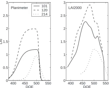
5.2. Vegetation data 5.2.1. Leaf Area Index
Leaf Area Index (LAI) was measured almost every week using a planimeter. In order to provide daily values, the data were fitted to a continuous function of time (see Eq. (11) in Appendix I). Measurements were also performed using LAI2000 (LiCOR) systems as soon as plant canopies were developed enough. Significant differences were noticed be-tween the two types of measurements, especially on fields 101 and 120 (Fig. 1). This was explained by the effect of stems and ears on LAI2000 measurements. LAI2000 mea-surements were time interpolated using spline functions. Planimetric measurements were used in Scenarios 1 and 2,
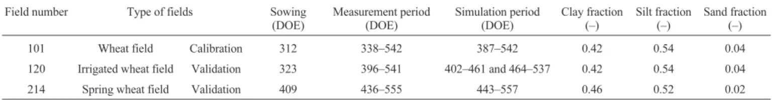
Table I. Field references, measurement periods (including all types of continuous measurements) and simulation periods.
Field number Type of fields Sowing
(DOE) Measurement period (DOE) Simulation period (DOE) Clay fraction (–) Silt fraction (–) Sand fraction (–)
101 Wheat field Calibration 312 338–542 387–542 0.42 0.54 0.04
120 Irrigated wheat field Validation 323 396–541 402–461 and 464–537 0.42 0.54 0.04
while in Scenario 3, modelers had the possibility of using ei-ther type of measurements.
5.2.2. Fraction of vegetation cover
The fraction of vegetation cover (veg) was used for parti-tioning latent heat flux and conduction heat flux between vegetation and soil in ISBA. It was calculated as a function of LAI:
veg = 1 – exp( –δLAI) (1)
where the extinction coefficient δ= 0.6. Similar equations
were used in the other models for partitioning net radiation
(with δ= 0.2 for MAGRET and δ= 0.4 for SiSPAT and
SOIL).
5.2.3. Vegetation height and aerodynamic parameters
Vegetation height (hc) was measured every week. A linear
interpolation was done between the measurements.
Rough-ness length for momentum, zom, roughness length for heat, zoh,
and displacement height d were derived from the vegetation height using simple expressions:
z h d h kB z z om c c om oh =013. ; =0 63. and –1 =ln =4. (2) These values were confirmed by measurements on field 120
(Zhao et al. [41] in this volume). The kB–1
value was derived from the data from a wheat experiment in La Crau in 1987 and 1988 (L. Prévot, personal communication). For bare soil
a typical value of 0.001 m was assigned to zom.
5.2.4. Albedo and emissivity
•In Scenario 1, albedo was derived from measurements
of reflected solar radiations on every calibration and valida-tion field (see François et al. [20] in this volume). Values at
maximum LAI were used for defining vegetation albedo or canopy albedo (0.22). For bare soil, an albedo of 0.23 was ob-served in dry conditions (soil moisture in the 0–5 cm layer
lower than 0.05 m3
·m–3
) and of 0.08 for wet conditions (soil
moisture in the 0–5 cm layer higher than 0.32 m3·m–3).
•In Scenario 2, we used a classical value for vegetation
albedo (0.23), and values obtained for a similar type of soil by
[31]: 0.10 for wet soil (surface soil moisture > 0.3 m3
·m–3
)
and 0.25 for dry soil (surface soil moisture < 0.1 m3
·m–3
).
•The measured values of emissivities were in agreement
with those classically used in the different models. The vege-tation value (0.98) and soil value (0.96) were used in all sce-narios.
5.2.5. Stomatal conductance
•In Scenario 1, the maximum measured value of stomatal
conductance was used: 0.0062 m·s–1
equivalent to
rsmin= 161.2 m·s
–1
(LiCOR 6400 instrument). This value was representative of a mildly water-stressed crop. Then, some tests were also performed using the more classical value of
0.020 m·s–1
. This last value was also used in Scenario 2.
•Other parameters in stomatal conductance calculations
were set to their traditional values in each model (Scenarios 1
and 2). When possible, standard values such as 1/5000 m·s–1
for minimum conductance, –140 m or –1.4 Mpa for critical leaf water potential and 40 hPa for vapor pressure deficit at full stomatal closure were used. This was done for SiSPAT and ISBA but differences existed for MAGRET, in which no effect of vapor pressure deficit was included during this study, and SOIL, which used a different type of equation for computing stomatal resistance.
5.2.6. Root depth and density
The evolution of rooting depth during crop cycles was es-timated from the evolution of soil moisture profiles (see Fig. 12 in Olioso et al. [32], this volume). Direct measure-ments of root density were added to these observations. This information was used as input for SiSPAT and SOIL. The maximum rooting depth was also used for defining the depth of the simulated soil column in each model: 2 m for field 101 and 1.4 m for fields 120 (irrigated) and 214 (spring wheat).
5.3. Soil parameters, initial and boundary soil conditions
Depending on the model, inputs describing soil processes were very different. For instance, complex models such as SiSPAT and SOIL required a fine description of the hydro-dynamical properties of the soil, while models such as MAGRET and ISBA only required wilting point and field ca-pacity (in these models, other parameters required for de-scribing water transfers in the soil were internally computed as a function of soil texture). A detailed description of the soil of some of the fields was done during the experiment [32]. This included measurements of texture, dry bulk density, profiles of soil moisture and soil water potential, soil
400 450 500 550 0 0.5 1 1.5 2 2.5 3 LAI DOE Planimeter 101 120 214 400 450 500 550 0 0.5 1 1.5 2 2.5 3 DOE LAI2000
Figure 1. Interpolated LAI measurements on wheat fields 101, 120 and 214, obtained using a planimeter (left graph) or LAI2000 system (right graph).
temperature profiles, hydraulic conductivity, apparent ther-mal conductivity and retention curves. From these measure-ments it was possible to derive the information required by the different models. A description of these derivations may be found in [3]. The main points are outlined in the following paragraphs and in Appendix I.
5.3.1. Layer definition
The horizontal discretization of soil was done according to vertical variations of soil dry bulk density and texture: 1 to 4 soil layers were defined depending on the fields. Soil prop-erties were affected in the different soil layers and were used as inputs in SiSPAT and SOIL. For ISBA, MAGRET and SiSPAT-h, uniform soil properties were defined by ‘averag-ing’ basic soil properties over the whole simulated column. In Scenario 2, soil was assumed to be vertically uniform.
5.3.2. Retention curves
In SOIL and SiSPAT retention curves were described by the model proposed by Van Genuchten [38]:
θ θ θ θ – – – r s r g n m h h = + 1 (3)
whereθis the volumetric soil moisture,θrits residual value
and θsthe soil moisture at saturation; h is the soil water
po-tential, hg, n and m three empirical parameters. In Scenario 1,
equation (3) was fitted on the measured data, while in Sce-nario 2, it was derived by using the pedotransfer functions from [34]. In the case of SiSPAT for Scenario 1, a modifica-tion of the Van Genuchten equamodifica-tion was introduced in order to account for dry conditions which were outside of the range of the measurements, i.e. for potential lower than –100 m. This modification was done using the methodology proposed by [35]. The retention curves derived for a homogeneous soil column in the 3 fields and Scenarios 1 and 2 are presented in Figure 2. A more detailed description of fitting procedures and the values of the fitted parameters for each layer are given in Appendix I.
Retention curves were used to define field capacity (h = –3.3 m) and wilting point (h = –150 m), parameters which were required in the bulk soil descriptions included in ISBA and in MAGRET (see Tab. II, Fig. 2 and Appendix I).
5.3.3. Hydraulic conductivity
•In Scenario 1, hydraulic conductivity was expressed as a
function of soil moisture using the Brooks and Corey model:
K Ksmat s ( )θ θ θ η = (4)
• The two parametersηand Ksmatwere obtained from
lab-oratory measurements on soil samples from some fields (see Tab. II and Appendix I). However, in situ estimations of
satu-rated hydraulic conductivity Ksgave values several order of
magnitude higher than Ksmat(Tab. II). This was explained by
the existence of macroporosities. A modification of the Brooks and Corey model was proposed to account for this macroporosity (see Appendix I).
• In Scenario 2 we used the pedotransfer functions from
[34] applied to the Van Genuchten model (see Appendix I). A comparison of the hydraulic conductivity derived in Sce-narios 1 and 2 is presented in Figure 3.
0 0.1 0.2 0.3 0.4 0.5 0.5 1 1.5 2 2.5 3 3.5 4 Field capacity Wilting point
Volumetric soil moisture
log10(|soil w
ater potential|) (log10(|m|))
Scenario 1 Scenario 2
Figure 2. Retention curves derived for wheat fields in Scenarios 1 and 2, assuming a homogeneous soil column.
Table II. Soil properties directly derived from the measurements on wheat fields in Scenario 1 and derived from texture data and pedotransfer functions in Scenario 2 (θsis the soil moisture at saturation; Ksmatis the saturated hydraulic conductivity obtained in the laboratory on soil
sam-ples; Ksis the saturated hydraulic conductivity estimated in situ (Scenario 1) or using the pedotransfer function (Scenario 2)).
Scenario 1 Scenario 2
Field number
Depth (cm)
Dry bulk density
(g·cm–3) θ s (m3·m–3) Wilting point (m3·m–3) Field capacity (m3·m–3) Ksmat (m·s–1) Ks (m·s–1) Dry bulk density (g·cm–3) θs (m3·m–3) Wilting point (m3·m–3) Field capacity (m3·m–3) Ks (m·s–1) 101 0–200 1.60 0.37 0.239 0.362 5.0 × 10⁻⁹ 2.4 × 10⁻⁶ 1.45 0.453 0.248 0.382 2.558 × 10⁻⁸ 120 0–140 1.54 0.38 0.239 0.368 1.0 × 10⁻⁹ 2.4 × 10⁻⁶ 1.40 0.473 0.246 0.388 4.400 × 10⁻⁸ 214 0–140 1.46 0.39 0.241 0.368 5.0 × 10⁻⁹ 3.0 × 10⁻⁶ 1.40 0.473 0.265 0.401 2.735 × 10⁻⁸
5.3.4. Heat capacity
The volumetric heat capacity was computed as: Ch d ( ) . . . θ =2 0 10× ρ + × θ 2 65 418 10 6 6 . (5)
In Scenario 1, the dry bulk densityρdwas obtained from
mea-surements. In Scenario 2, it was obtained from [34] pedotransfer functions.
5.3.5. Thermal conductivity
• For Scenario 1, thermal conductivity measurements
were used to adjust a single equation based on the model pro-posed by [25]: λ θ θ θ θ θ ( ) . . . – exp – . . = + + 0 492 0 734 0 303 1 34 54 3 82 s s (6)
(all the measurement points from all fields and depths were used together).
• In Scenario 2, we used the method proposed by [37] for
computing thermal inertia from soil class. Then, we derived the conductivity as:
λ θ θ θ ( ) ( ) . ( ) . = + 1 1 0 654 550 2300 2 Ch (7)
• However, it must be noticed that different equations
were used in MAGRET and SOIL. All these equations are presented, together with the in situ measurements, in Figure 4.
5.4. Initial and boundary conditions for temperature and moisture
• In Scenario 1, when possible, measurements of soil
moisture, soil matrix potential and temperature profiles were
used as initial conditions. When the soil depth was 2 meters (field 101), no measurements were available and a low matrix potential was assumed (h = –0.1 m). In the case of SiSPAT, this boundary condition was generating large unrealistic cap-illary rises and a gravitational flow was used instead. Soil temperature at the bottom of the soil column was given by a sinusoidal function of day which was fitted on temperature measurements on the meteorological site (see [3]).
• In Scenario 2, as simulations started just after the rainy
period, we assumed that the fields were at field capacity and that the soil matrix potential was constant with depth. Soil temperature profiles were initialized using a linear relation between the deep temperature and the air temperature at mid-night. For bottom conditions we assumed constant soil matrix potentials (the same as for the initial value) and soil moistures derived using the retention curves.
6. COMPARISON OF OUTPUTS
Model simulations were compared to measurements in or-der to globally assess their precision. The root Mean Squared Errors (RMSE), Bias (B) and Nash index (NI) were computed for the only outputs that were common to all the models: en-ergy balance fluxes Rn, H, LE and G and integrated soil mois-ture over the simulation depth.
RMSE n i si mi n = =
∑
1 2 1 ( – ) ; (8) B n i si mi n = =∑
1 1 ( – ); (9) 0 0.1 0.2 0.3 0.4 0.5 10 15 20 25 30 35Volumetric soil moisture
log10(h
ydr
aulic conductivity)
Scenario 1 Scenario 2
Figure 3. Hydraulic conductivity as a function of soil moisture in Scenarios 1 and 2, assuming a homogeneous soil column.
0 0.2 0.4 0.6 0.8 1 1.2 1.4 1.6 1.8 2 Ther mal Conductivity (W/m/K) 0.05 0.1 0.15 0.2 0.25 0.3 0.35 0.4 0.45
Volumetric Soil Moisture
measurements 5cm measurements Scenario1 Scenario2 Magret SOIL 0.5 * Scenario1
Figure 4. Thermal conductivity measurements and models as a func-tion of soil moisture. Measurements in the 5 first centimeters were sorted out. The conductivity obtained by dividing the conductivity computed in Scenario 1 by 2 is also presented.
NI s m m m i i i n i i i n = < > = =
∑
∑
1 2 1 2 1 – ( – ) ( – ) (10)where siis a model result, mithe associated measurement and
n the number of available data.
The Nash Index expresses the efficiency of the model at reproducing the considered variable in comparison with its
mean measured value <mi>. A value of NI close to 1
corre-sponds to a very good simulation of the variable, while a value of NI close to zero shows that the simulation is not per-forming better than simply using the mean measured value of the variable. A negative value expresses an even worse simu-lation. The RMSE, B and NI were computed either for the whole data set, or for each field separately.
Flux and soil moisture data have been presented by Olioso et al. [32] in this issue. However, note that H was measured using the eddy-correlation system and that LE was derived from the energy balance equation and the measurements of H, Rn and G. The soil moisture data used in this study were ob-tained from neutron probe measurements down to 1.4 m.
7. RESULTS FOR THE DIFFERENT VARIABLES IN SCENARIOS 1 AND 2
Comparison of the models’ outputs with measurements in Scenarios 1 and 2 are presented in Tables III and IV and Fig-ures 5 to 8.
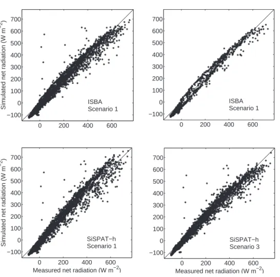
Net radiation Rn was always well simulated since NI val-ues very close to 1 were obtained (Tabs. III and IV and Fig. 5). The values of RMSE were low and in the same range as measurement errors. Variations between models were low. It is, however, possible to notice that the more complex mod-els usually presented a larger RMSE than ISBA, in which a constant value of albedo was given for the whole set of simu-lations. This shows that introducing complex interactions, such as the dependence of soil albedo on surface soil moisture (SiSPAT and SOIL) or the dependence of albedo on the solar zenith angle (SiSPAT and MAGRET), was not improving surface energy balance simulations (however, it is possible that the partition of energy between vegetation and soil was better simulated). Not much difference was found between Scenario 1 and Scenario 2. It must also be noticed that a part of the difference between models and measurements was ex-plained by the distance between the central meteorological station, in which incoming radiations were measured, and the experimental fields, where net radiation data were acquired. This was really significant for field 101 which was 1.8 km away (field 120 and field 214 were closer, 600 m and 750 m, respectively). When cloudy days were dropped from the comparison, the simulations were closer to the measurements (Fig. 5). It must be noticed that surface temperature simula-tions (not shown) were always rather good (RMSE lower than 2 K) and did not affect net radiation simulations on a large extent.
Ground heat flux G: NI were mostly bad in Scenarios 1 and 2 except for MAGRET and SOIL. RMSE values were also large for the other models and in particular for both ver-sions of SiSPAT. They were larger than the errors we can Table III. SVAT model results on wheat fields (all together) for Scenarios 1 and 2. Case A corresponds to Scenario 1 with a modified minimum stomatal resistance.
Rn (W·m–2) H (W·m–2) LE (W·m–2) G (W·m–2) Soil moisture (m3·m–3)
Number of data 9430 2089 2086 9480 50
ISBA RMSE B NI RMSE B NI RMSE B NI RMSE NI RMSE B NI
Scen. 1 33 –8 0.97 71 15 0.27 75 –28 0.50 43 0.12 0.024 0.013 0.54
Case A 33 –7 0.98 59 6 0.50 62 –17 0.65 42 0.16 0.018 0.004 0.76
Scen. 2 33 –9 0.97 70 –7 0.29 76 –6 0.48 46 –0.02 0.028 0.021 0.38
MAGRET RMSE B NI RMSE B NI RMSE B NI RMSE NI RMSE B NI
Scen. 1 39 –18 0.97 40 9 0.77 64 –31 0.63 26 0.69 – – –
Scen. 2 43 –19 0.96 35 –16 0.82 42 –2 0.84 22 0.77 – – –
SOIL RMSE B NI RMSE B NI RMSE B NI RMSE NI RMSE B NI
Scen. 1 40 –22 0.96 45 9 0.71 66 –34 0.60 34 0.43 0.040 0.030 –0.24
Case A 41 –22 0.96 37 –9 0.81 49 –17 0.78 34 0.43 0.028 0.016 0.40
Scen. 2 44 –25 0.96 38 –14 0.80 48 –13 0.79 37 0.34 0.040 0.033 –0.22
SiSPAT RMSE B NI RMSE B NI RMSE B NI RMSE NI RMSE B NI
Scen. 1 37 –4 0.97 44 18 0.72 56 –25 0.72 51 –0.24 0.026 0.022 0.44
Scen. 2 40 –4 0.96 48 14 0.67 60 –19 0.67 70 –1.36 0.026 0.028 0.48
SiSPAT–h RMSE B NI RMSE B NI RMSE B NI RMSE NI RMSE B NI
Scen. 1 38 –5 0.97 40 8 0.77 53 –16 0.75 62 –0.87 0.021 0.014 0.66
expect for that type of measurement. Figure 6 shows that a large overestimation of the daily flux amplitude usually oc-curred for ISBA and SiSPAT. It was clear that equations (6) and (7) used in Scenarios 1 and 2 were not adequate for simu-lating fluxes in agreement with measurements. The functions used in MAGRET and SOIL gave slightly lower conductivity values than the two other equations (Fig. 4), but this may not be a definitive explanation of the better simulations. The way heat transport in the soil was calculated in these two models may also be part of the explanation. As a matter of fact, the thickness of the layers used in the discretization for solving the Fourier equation was 2.5 cm for SOIL and 10 cm for MAGRET, while it was about 1 or 2 mm in SiSPAT. There-fore, temperature gradients may be very different, generating large differences in fluxes. ISBA had a behavior close to
SiSPAT, which was logical since the equations used in the force restore method for ground temperature were originally derived from a detailed treatment of ground heat flux [15, 30]. Also, note that thermal conductivity measurements used for fitting equation (6) were done from some centimeters be-low the soil surface down to 50 cm. It is therefore possible that they were not representative of the real surface proper-ties. As a matter of fact, Figure 4 shows that the closest mea-surements to the surface (at 5 cm) may have a very low conductivity value compared with conductivity models. Ex-cepted for SiSPAT, no large difference existed between Sce-narios 1 and 2, even if a slight degradation of the results usually occurred. The thermal conductivity model in Sce-nario 2 generated higher values than the equation used in Scenario 1, and then higher overestimations of ground heat Table IV. SVAT model results on wheat fields for Scenarios 1 and 3 (calibration and validation). Case A corresponds to Scenario 1 with a modi-fied minimum stomatal resistance.
Rn (W·m–2) H (W·m–2) LE (W·m–2) G (W·m–2) Soil moisture (m3·m–3)
Number of data
Field 101 3713 1112 1112 3689 19
Field 120 3132 295 293 3132 16
Field 214 2585 682 681 2659 15
ISBA RMSE B NI RMSE B NI RMSE B NI RMSE NI RMSE B NI
Field 101–Scen. 1 38 –16 0.96 73 19 –0.21 76 –37 0.46 43 0.08 0.031 –0.020 0.562 Field 101–Case A 38 –16 0.96 60 9 0.19 61 –25 0.65 42 0.13 0.021 –0.012 0.802 Field 101–Calibration 36 –14 0.97 45 –5 0.54 46 –3 0.80 32 0.50 0.022 –0.014 0.776 Field 120–Scen. 1 27 0 0.98 88 25 0.22 93 –39 0.52 37 0.26 0.015 –0.003 0.707 Field 120–Case A 27 1 0.98 65 7 0.58 75 –19 0.69 36 0.31 0.014 0.011 0.732 Field 120–Validation 28 4 0.98 90 –31 0.20 113 31 0.30 28 0.57 0.010 0.006 0.869 Field 214–Scen. 1 34 –5 0.98 60 4 0.64 63 –8 0.55 49 0.03 0.022 –0.015 0.179 Field 214–Case A 33 –5 0.98 56 1 0.68 57 –4 0.63 48 0.05 0.016 –0.010 0.562 Field 214–Validation 33 –3 0.98 44 –2 0.80 37 6 0.76 33 0.56 0.014 –0.010 0.682
SiSPAT RMSE B NI RMSE B NI RMSE B NI RMSE NI RMSE B NI
Field 101–Scen. 1 41 –14 0.96 45 20 0.55 51 –31 0.75 51 –0.32 0.025 –0.021 0.714 Field 101–Case A 41 –13 0.96 28 –5 0.82 32 –2 0.91 50 –0.24 0.013 –0.010 0.927 Field 101–Calibration 40 –9 0.96 33 –6 0.76 31 5 0.91 30 0.55 0.007 –0.003 0.978 Field 120–Scen. 1 34 9 0.98 59 25 0.65 77 –34 0.68 52 –0.43 0.021 –0.019 0.363 Field 120–Validation 34 14 0.97 68 6 0.54 74 3 0.70 34 0.37 0.010 –0.006 0.851 Field 214–Scen. 1 34 –6 0.98 34 10 0.88 51 –13 0.70 50 0.00 0.022 –0.029 –0.721 Field 214–Validation 35 4 0.98 23 –1 0.95 37 5 0.85 34 0.52 0.014 –0.012 0.681
SiSPAT–h RMSE B NI RMSE B NI RMSE B NI RMSE NI RMSE B NI
Field 101–Scen. 1 44 –11 0.95 37 12 0.70 50 –21 0.77 67 –1.22 0.015 –0.007 0.902 Field 101–Calibration 34 –9 0.97 40 –2 0.64 43 –4 0.82 27 0.64 0.027 0.026 0.670 Field 120–Scen. 1 33 7 0.98 58 15 0.66 69 –29 0.74 54 –0.59 0.027 –0.020 0.011 Field 120–Validation 27 10 0.98 61 –27 0.63 75 29 0.69 21 0.77 0.025 –0.019 0.107 Field 214–Scen. 1 36 –10 0.97 36 –2 0.87 50 –2 0.72 65 –0.71 0.020 –0.016 0.348 Field 214–Validation 38 5 0.97 67 –43 0.54 100 66 0.13 36 0.49 0.007 0.002 0.926
flux were obtained. The effect of the simulation of surface soil moisture and temperature gradients may also have an in-fluence. However, as shown for SiSPAT and SiSPAT-h, there were only very little changes in surface moisture simu-lations between Scenarios 1 and 2 (Fig. 7).
Heat fluxes H and LE: in Scenario 1, H was almost al-ways overestimated and LE underestimated (Tabs. III and IV and Fig. 8). A significant part of the RMSE for LE was usu-ally explained by a large bias. This is also the case, but to a lesser extent, for H. We must notice that the measurements of H were performed in the field using both eddy-correlation systems and Bowen ratio systems (only eddy-correlation data were used in the present study). The comparison of the two sets of measurements by [32] showed that H measured with the eddy-correlation method underestimated Bowen ratio measurements by around 10% and that a large dispersion
oc-curred (Root mean square differences around 70 W·m–2
). In Scenario 2, the Bias and RMSE of LE were reduced in com-parison with Scenario 1 for MAGRET and SOIL. For ISBA, RMSE were almost constant while Bias were significantly different (actually, when looking at the results field by field, the RMSE for ISBA decreased, by the same amount as for the other models, in fields 101 and 120, but a large increase
occurred in field 214). For SiSPAT, the RMSE increased from Scenario 1 to Scenario 2. A great difference between Scenario 2 and Scenario 1 may be found in the prescribed
value for the minimum stomatal resistance (50 s·m–1
instead
of 161.2 s·m–1
). This may explain improvements in simulat-ing LE. Some tests were performed by changsimulat-ing the mini-mum stomatal resistance but keeping all the other inputs as they were prescribed in Scenario 1 (Case A in Tabs. III and IV). For each of these tests, large improvements in the results were obtained for LE and H, even for ISBA and SiSPAT (this last model was only tested on field 101). For SiSPAT, the re-sults in Scenario 2 were affected by other factors which had counter-balanced improvements due to changing stomatal conductance.
•There was a degradation of the validity of hydrodynamic
parameters from Scenario 1 to Scenario 2 in which pedotransfer functions were used. Retention curves were very similar in the agronomic range, but large differences occurred in the dry part for potentials lower than wilting point (Fig. 2). Hydraulic conductivity was some order of magnitude lower in Scenario 2 than in Scenario 1 (Fig. 3). This had significantly reduced water transfers and then evapotranspiration. 0 200 400 600 −100 0 100 200 300 400 500 600 700
Simulated net radiation (W m
−2 ) ISBA Scenario 1 0 200 400 600 −100 0 100 200 300 400 500 600 700 ISBA Scenario 1 0 200 400 600 −100 0 100 200 300 400 500 600 700
Measured net radiation (W m−2)
Simulated net radiation (W m
−2 ) SiSPAT−h Scenario 1 0 200 400 600 −100 0 100 200 300 400 500 600 700
Measured net radiation (W m−2) SiSPAT−h Scenario 3
Figure 5. Examples of compari-son between simulations of net radiation and measurements on field 101. The top right graph was obtained without cloudy data.
•Saturated water content also presented higher values in Scenario 2. This had a great influence on initial soil water content and then on simulation of H, LE and soil moisture. This was particularly true for field 214 (Fig. 9 and Tab. II).
•The horizontal description of soil for SiSPAT was
de-graded (since Scenario 2 considered an homogeneous soil column).
•The simulations of ground heat flux were also degraded.
For models with a simple description of soil (ISBA and MAGRET), as the hydrodynamic properties were almost un-changed between Scenarios 1 and 2, the improvement of sim-ulation linked to the change in stomatal resistance was not counterbalanced. However, on field 214, ISBA simulations were affected by the large change in initial soil moisture. This was also the case for MAGRET but to a lesser extent. It must be noticed that for this field, LAI was always very low (lower than 1), and that mono-layer energy balance models may
−100 0 100 200 −150 −100 −50 0 50 100 150 200 250
Simulated soil heat flux (W m
−2 ) MAGRET Scenario 1 −100 0 100 200 −150 −100 −50 0 50 100 150 200 250 SOIL Scenario 1 −100 0 100 200 −150 −100 −50 0 50 100 150 200 250
Simulated soil heat flux (W m
−2 ) SiSPAT Scenario 1 −100 0 100 200 −150 −100 −50 0 50 100 150 200 250 SiSPAT Scenario 3 −100 0 100 200 −150 −100 −50 0 50 100 150 200 250
Measured soil heat flux (W m−2)
Simulated soil heat flux (W m
−2 ) ISBA Scenario 1 −100 0 100 200 −150 −100 −50 0 50 100 150 200 250
Measured soil heat flux (W m−2) ISBA
Scenario 3 Figure 6. Examples of compari-son between simulations of ground heat flux and measure-ments on field 101.
have difficulties simulating turbulent exchanges and soil evaporation in this situation.
Soil moisture: the results were very similar to the results obtained with LE. When LE was underestimated, an overesti-mation of soil moisture was noticed. The test of a lower mini-mum stomatal resistance in Scenario 1 (case A) improved the simulation of total soil moisture. This was not always noticed in Scenario 2, in which other processes had to be taken into account, such as the differences in soil hydrodynamic proper-ties.
8. SCENARIO 3: CALIBRATION/VALIDATION The third scenario was implemented only for ISBA and both SiSPAT versions. A calibration of the models was done on field 101. It aimed to improve the simulations of energy balance and soil moisture. The choice of a calibration proce-dure was left free for the modelers. All of them manually
changed the value of some of the parameters that were known to have an impact on the simulations. After being calibrated, the models were tested on fields 120 and 214 in order to as-sess the robustness of the calibration process: on these two fields, parameters were changed in the same manner as they were changed on field 101.
For the three models, the first calibration step consisted of improving the simulation of ground heat flux. The thermal conductivity was strongly reduced: it was multiplied by 0.3 for ISBA and by 0.5 for the two versions of SiSPAT (Fig. 4). This was done only in the top soil layer for the normal SiSPAT version and over the whole soil profile for the homo-geneous version. Simulations of ground heat flux were highly improved in all fields (Tab. IV and Fig. 6).
Also in order to improve available energy simulations, in both SiSPAT versions, some modifications were made in the simulation of albedo and radiation partition between the soil and the vegetation. In some cases, the response of soil albedo to surface soil moisture was slightly modified (this was par-ticularly done to improve albedo when the vegetation cover was low, as in field 214). For the homogeneous SiSPAT ver-sion, LAI measured by means of a LAI2000 instrument were used for radiative and aerodynamic processes instead of planimetric measurements (for the calculation of surface re-sistance, the planimetric measurements were still used). LAI2000 provided higher values of LAI because it included the effect of stems and ears (Fig. 1). This modification was done in order to improve the simulation of net radiation, and also to increase the absorption of radiation by the vegetation layer. For this scenario, the absorption of solar radiation was computed using the SAIL radiative transfer model (as done by [16, 17, 31]). In Scenarios 1 and 2, radiation absorption was computed by means of a simple Beer-Lambert exponen-tial description. A great improvement in net radiation simula-tion was obtained for field 101 (Fig. 5 and Tab. IV). The improvement was less in field 120. No improvement was found for field 214 for which the modification of LAI was low (Fig. 1). As the solar radiation reaching the soil was lower, the increase in LAI may have an influence on the improve-ment of ground heat flux simulation with SiSPAT-h (Tab. IV). The same behavior was noticed for ISBA in simu-lations considering a higher vegetation cover (set to 0.8 at its maximum, while it never exceeded 0.5 in Scenario 1) (results not shown). It may also be possible that increasing LAI helped to improve the simulation of latent heat flux through an increase of the available energy for plant transpiration.
A third step in the calibration process consisted of improv-ing evapotranspiration and soil moisture simulations:
•In order to increase transpiration, the stomatal resistance
was decreased from 161.2 s·m–1
to 50 s·m–1
in both versions
of SiSPAT and to 40 s·m–1
in ISBA. In ISBA, the response of stomatal conductance to vapor pressure deficit was also deactivated.
•In order to have higher soil water transfers, hydraulic
con-ductivities were increased in both versions of SiSPAT. This also allowed the simulation of a faster drying of the
400 450 500 550 0.05 0.1 0.15 0.2 0.25 0.3 0.35 0.4 0.45 SiSPAT−h Day of Experiment Soil moisture (m 3 m −3 ) 400 450 500 550 0.05 0.1 0.15 0.2 0.25 0.3 0.35 0.4 0.45 Soil moisture (m 3 m −3 ) SiSPAT TDR measurements Scenario 1 Scenario 2 Scenario 3 400 450 500 550 0.05 0.1 0.15 0.2 0.25 0.3 0.35 0.4 0.45 SiSPAT−h Day of Experiment Soil moisture (m 3 m −3 ) 400 450 500 550 0.05 0.1 0.15 0.2 0.25 0.3 0.35 0.4 0.45 Soil moisture (m 3 m −3 ) SiSPAT TDR measurements Scenario 1 Scenario 2 Scenario 3
Figure 7. Surface soil moisture simulations on field 101 for both SiSPAT versions and for Scenarios 1, 2 and 3.
0 200 400 600 −100 0 100 200 300 400 500 600 SiSPAT Scenario 1 0 200 400 600 −100 0 100 200 300 400 500 600
Simulated latent flux (W m
−2 ) ISBA Scenario 1 0 200 400 600 −100 0 100 200 300 400 500 600 SiSPAT Scenario 1−A 0 200 400 600 −100 0 100 200 300 400 500 600
Simulated latent flux (W m
−2 ) ISBA Scenario 1−A 0 200 400 600 −100 0 100 200 300 400 500 600 SiSPAT Scenario 3 0 200 400 600 −100 0 100 200 300 400 500 600
Simulated latent flux (W m
−2 ) ISBA Scenario 3 0 200 400 600 −100 0 100 200 300 400 500 600
Measured latent heat flux (W m−2)
Simulated latent flux (W m
−2 ) MAGRET Scenario 2 0 200 400 600 −100 0 100 200 300 400 500 600
Measured latent heat flux (W m−2)
SOIL Scenario 1−A
soil surface (Fig. 7). In the normal version of SiSPAT (het-erogeneous), the hydraulic conductivity at saturation in the first soil meter was increased 100 times [0–40 cm] and 10 times [40–90 cm]. Since in the SiSPAT-h version, it was not possible to modify the conductivity layer by layer,
a different strategy was followed: the hydraulic conductiv-ity at saturation was multiplied by only 2, but at the same
time the parameter ηin equation (3) was decreased from
19.5 to 17.5. This last change made possible a greater in-crease in conductivity at low soil moisture, which usually
400 450 500 550 0.2 0.25 0.3 0.35 0.4 SiSPAT Field 101 400 450 500 550 0.2 0.25 0.3 0.35 0.4 ISBA Field 101 Soil moisture (m 3 m −3 ) Measurements Scenario 1 Scenario 2 Scenario 3 420 440 460 480 500 520 540 0.2 0.25 0.3 0.35 0.4 SiSPAT Field 120 420 440 460 480 500 520 540 0.2 0.25 0.3 0.35 0.4 ISBA Field 120 Soil moisture (m 3 m −3 ) 460 480 500 520 540 560 0.2 0.25 0.3 0.35 0.4 SiSPAT Field 214 Day of Experiment 460 480 500 520 540 560 0.2 0.25 0.3 0.35 0.4 ISBA Field 214 Day of Experiment Soil moisture (m 3 m −3 )
occurred closer to the soil surface. It must be noticed that
changingηaltered the structural link between the hydraulic
conductivity and the retention curve, and thus may have no physical meaning. For SiSPAT-h, the dry extension of the retention curve was also used to improve simulations of dry periods (it was not used in Scenario 1).
Stomatal conductance and hydraulic conductivity were the two main physical parameters which were used in the cal-ibration of evapotranspiration and soil moisture. Some other parameters were changed in order to have a finer tuning of the evolution of soil moisture profiles.
•In order to increase the availability of water for the plants,
the total plant resistance to water transfer was decreased
from 3.0× 10⁻¹²
s·m–1
to 10–12
s·m–1
in SiSPAT and SiSPAT-h. With the same objective, soil depth was in-creased to 3 m for field 101 and to 2 m for fields 120 and 214 in ISBA (these changes may be justified by the defini-tion of a soil depth that may exceed root depth in order to account for water transfers occurring below this depth, as proposed by [29, 30]).
•The changes in hydraulic conductivity affected the
reparti-tion of water in the different soil layers, and particularly near the soil surface. In ISBA, for which no profile really existed, field capacity was slightly decreased from
0.362 m3
·m–3
to 0.35 m3
·m–3
on field 101 and wilting point
was slightly increased from 0.239 m3
·m–3
to 0.25 m3
·m–3
(the modified values were also used on fields 120 and 214). In SiSPAT root density was decreased and a temporal vari-ation was introduced (maximum value was set to
1500 m·m–3
between DOE 387 and 420, 3000 m·m–3
be-tween DOE 420 and 450, and 6000 m·m–3
after DOE 450,
instead of a constant value of 10 000 m·m–3
). For SiSPAT-h a similar procedure was followed but with
dif-ferent values (maximum value was set to 500 m·m–3
on
DOE 387 and progressively increased to 9000 m3
·m–3
on DOE 527).
Simulations of LE, H and soil moisture were generally sig-nificantly improved when ISBA and SiSPAT models were calibrated (field 101): Table IV, Figure 8. For ISBA a first improvement in heat fluxes was linked to the decrease of the minimum stomatal resistance (Case A in Tab. IV). A second improvement was obtained thanks to changing the soil prop-erties.
For SiSPAT-h, even if latent heat flux was better simu-lated, this was not the case for soil moisture. Due to the mono-layer soil description, the calibration of SiSPAT-h was really difficult. It was not possible to simulate correctly evapotranspiration and the soil moisture profile at the same time (in particular, surface soil moisture at the same time as the integrated soil moisture over the root zone). Moreover, in the calibration process, a significant effort was made to im-prove the simulation of surface soil moisture, without de-grading the simulation of latent heat flux. This choice was made because the intention of the modelers using SiSPAT-h was to link the model to surface moisture as obtained from microwave remote sensing data in further studies (Demarty [16]). Figure 7 shows that the simulation of surface soil
mois-ture was improved with SiSPAT-h. It was also the case for the normal version of SiSPAT (Fig. 7), but for this model, as it was possible to modify the hydraulic conductivity respective to soil depth, the simulation of the total soil moisture and the simulation of latent heat flux were improved at the same time. When the parameters calibrated on field 101 (or similar changes in the way of setting the parameters) were applied to the two other fields, contradictory results were obtained: sim-ulation of soil moisture was mostly more accurate, while this was not always the case for latent and sensible heat fluxes. On field 120, these fluxes were almost never improved. On field 214, better simulations were obtained only with SiSPAT and ISBA. The degradation of the results was almost always linked to a large overestimation of latent heat flux. This shows that the type of changes made on field 101 for increas-ing evapotranspiration were too great to be applied to field 120, while they were adequate for field 214 in the case of ISBA and SiSPAT. The application of SiSPAT-h to field 120 and field 214 presented very different results in comparison with the normal version of SiSPAT. Once again, this illustrates the difficulties of managing at the same time surface soil moisture, root zone soil moisture and heat fluxes with the homogeneous version of SiSPAT.
9. CONCLUDING REMARKS
General comments may be made from the results pre-sented in this paper.
(i) The models’ results were close despite the large differ-ences existing in their parameterization and complexity level.
(ii) Better results were often obtained in Scenario 2 com-pared with Scenario 1, which may be surprising consid-ering the scenario definitions; however, this was due in great part to the change in minimum stomatal resistance. (iii) For the more complex model (SiSPAT), Scenario 2 did
not give better results. That may be due to the less
adequate hydraulic properties obtained by using
pedotransfer functions (mainly for hydraulic conductiv-ity). The portability of such models may be very low and it may be very difficult to apply them on situations where only little information on soil is available. Portability was better in the case of simple models in which only field capacity and wilting point were given as inputs. (iv) On the calibration fields, the results in Scenario 3 were
better than for the two other scenarios. Application to the validation fields did not always provide good results for turbulent heat fluxes, while better results were always obtained for G and nearly always for soil moisture. How-ever, if we look at the soil moisture, which is the most in-tegrating variable for this experiment, a model which was calibrated on a specific site may be successfully ap-plied to other sites with a quite similar soil type, showing that the calibration process was robust.
(v) The use of SiSPAT with an homogeneous soil column generated a lot of problems, showing that it may be
difficult to use this type of complex model without tak-ing into account soil layertak-ing.
Some results also questioned the data that were used in the definition of model inputs. First, due to the very dry condi-tions, the root system reached soil layers deeper than the depth investigated during the measurements. It was then dif-ficult to define boundary conditions and to assign parameter values in the deeper layers. Secondly, many points seemed to indicate that LAI values derived from planimetric measure-ments might have underestimated the vegetated surfaces wich have an influence on radiative and heat exchanges with the atmosphere: (i) LAI2000 measurements gave better re-sults in radiative transfer calculations; (ii) ISBA simulations with a very high vegetation cover parameter (not shown) gave very good results compared with the nominal Sce-nario 1; (iii) for each model, calibration in SceSce-nario 3 re-quired that water transfer efficiency was increased. Once again, the particular water conditions during the experiment might be responsible for such problems, since vegetation de-velopment was depressed, inducing low leaf surfaces and then enhancing the effect of stem and ear surfaces on energy exchanges. Such effects had been demonstrated during sev-eral experimental works on the adaptation of durum wheat to water stress and drought by [5, 10]. Thirdly, results on the ground heat flux suggest that the measurements of thermal conductivity may not be representative of the top soil layer (however, interaction with vegetation cover might have an effect on G).
The results obtained in this study provided a first insight into the potential use of our SVAT models for assimilating re-mote sensing data. It first appeared that there may be no inter-est in using the more complex models in such a domain, at least for monitoring energy and water fluxes. As a matter of fact, most of the assimilation procedures that have been pro-posed recently [8, 11, 19, 39] consist of sequential or variational retrievals of initial water content, methods that may not work properly when they use a model which is very sensitive to some unknown parameters, as is the case for the hydrodynamic properties in SiSPAT. With another point of view, work by [6], using passive microwave data and a com-plex soil model, showed that it may be possible to retrieve the hydraulic properties of top soil layers and then surface soil moisture. Similar results were obtained by [1] using radar data. However, it was unclear whether such studies could be extended to surfaces covered by vegetation in which water transfers also depend on deeper soil layers, as was the case in our study. Here, we tried to simplify the use of such complex models by considering a homogeneous soil column. This did not provide a solution to that problem. On the contrary, it ap-peared that simpler models (e.g. ISBA), which were more ro-bust toward the setting of soil parameters, may be more suitable for that type of assimilation technique. However, such models did not always simulate surface soil moisture (MAGRET) or the simulated surface soil moisture for a layer was not always well defined [9]. [39] showed that this may be the case for ISBA either because variation in soil hydraulic parameters may occur near the soil surface, or because the surface layer used in the force restore equation for soil
mois-ture is actually a very thin layer (some millimeters as defined by [30]). A solution proposed by [16] was to choose an arbi-trary soil layering, such as [0–10 cm], [10–30 cm] and [30–200 cm], that may account for usual agricultural prac-tices for soil preparation (ploughing and sowing) and their ef-fect on soil physical properties.
Acknowledgments: The Alpilles-ReSeDA project is funded by the EEC-DG XII (contract ENV4-CT96-0326-PL952071), the French Programme National de Télédétection Spatiale and Programme de Recherches en Hydrologie. Albert Olioso also thanks L. Léonard for her patience and support.
APPENDIX 1: PROTOCOL FOR TESTING SVAT MODELS
A.1. Vegetation data
Leaf Area Index as a function of DOE:
LAI DOE M a DOE t M b DOE t i s ( ) exp(– ( – ))– exp(– ( – )) = + + 1 1 (11)
where M, a, b, tiand tsare empirical parameters estimated by
non-linear fitting.
A.2. Soil parameters, initial and boundary soil conditions
A.2.1. Retention curves in Scenario 1
The model proposed by [38] given in equation (3) was fit-ted on the data set.
• θrthe residual soil moisture was always set to zero in
Sce-nario 1.
• θsthe soil moisture at saturation was determined from soil
moisture measurements when saturated conditions oc-curred. In some fields this was not possible and a function relating saturated water content to particle size distribution and soil dry bulk density was used [2, 21].
•The shape parameter m was determined from the particle
size distribution [2, 21, 40].
•Following the Burdine hypothesis n was related to m by
m = 1 – 2/n.
•Finally, hgwas fitted by eye on the data combining pressure
chamber measurements, in situ measurements of moisture and matrix potential and WIND laboratory measurements. To account for dry conditions (potential lower than –100 m) the procedure proposed by [35] was used to derive the following equation:
θ θs g n m g n h h h h = + + 1 1 2 2 2 2 2 0 – – – m2 (12)
•h0= – 60 000 m (at this tension, the water content was very
•m2= – 1 + 2/n2;
•Parameters n2 and hg2 were determined using the
New-ton-Raphson method and assuming continuity and derivability of equations (3) and (12).
Equation (12) was valid for h hc= –100 m while
equa-tion (3) was valid for h > hc.
This extension was not used in Scenario 1 for SOIL and for SiSPAT-h.
Fitted parameters are presented in Table V. A.2.2. Retention curves in Scenario 2
We used the pedotransfer functions from [34] to compute the coefficients in equation (3) as functions of granulometric data (conversely to Scenario 1 this was done assuming m = 1 – 1/n). A 1% organic matter content was assumed for the derivation of the dry bulk density.
Fitted parameters are presented in Table VI. A.2.3. Hydraulic conductivity in Scenario 1
The model proposed by Brooks and Corey (Eq. (4)) was
fitted on the data. The shape parameterηwas computed from
the particle size distribution [3, 21]. Then, only the saturated
conductivity corresponding to the soil matrix, Ksmat, was
fit-ted on the measurements for fields 101, 203 and 102 (WIND method). For other fields, values were assigned according to
the similarity in dry bulk density between measured and un-measured sites.
To account for discrepancies between Ksmatand in situ
esti-mations of saturated hydraulic conductivity Ks using
infiltrometers and a simplified infiltration test, a modifica-tion of the Brooks and Corey model was proposed to account
for macroporosity whenθs–θmacroⱕθⱕθs(withθmacrothe
macropore content):
log ( )K – s [logK – log (K – )] logK
macro s s macro s θ θ θ θ θ θ = + (13)
Equation (4) was only valid forθ ≤θs–θmacro. However, in
models like SiSPAT, the macroporosity extension was dropped for the deepest layers of the soil because it was gen-erating very large and unrealistic capillarity rises in some conditions. Fitted parameter values are presented in Table V.
A.2.4. Hydraulic conductivity in Scenario 2
The pedotransfer functions from [34] were applied to the Van Genuchten model leading to the following equation:
K Ks r r r r m ( ) – – – – – – / / θ θ θ θ θ θ θ θ θ = s s 1 2 1 1 1 m 2 (14)
Fitted parameters are given in Table VI.
Table V. Scenario 1: soil properties derived from the measurements on wheat fields: dry bulk density, retention curves and hydraulic conductiv-ity parameters.
Field number
Depth (cm)
Dry bulk density
(g·cm–3) (m3θ·ms–3) m (–) n (–) hg (m) m2 (–) n2 (–) hg2 (m) η (–) Ksmat (m·s–1) Ks (m·s–1) (m3macro·m–3) 101 0–10 1.3 0.43 0.0626 2.133 –0.4 0.05386 2.1138 –84.5 18.97 5.0×10⁻⁹ 7.0×10⁻⁶ 0.013 101 10–40 1.35 0.41 0.06373 2.136 –0.8 0.06048 2.1287 –86.4 18.67 1.8×10⁻⁹ 2.4×10⁻⁶ 0.013 101 40–90 1.6 0.383 0.05231 2.1103 –3.0 0.0942 2.208 –125.7 22.30 5.0×10⁻⁹ 2.0×10⁻⁶ 0.013 101 90–200 1.68 0.366 0.06153 2.131 –2.0 0.07591 2.164 –99.3 19.27 6.4×10⁻⁹ 2.75× 10⁻⁶ 0.036 101 0–200 1.6 0.37 0.06044 2.1286 –5.0 0.09503 2.21 –111.5 19.57 5.0×10⁻⁹ 2.4×10⁻⁶ 0.013 120 0–140 1.54 0.38 0.0601 2.128 –4.0 0.0905 2.199 –109.7 19.68 1.0×10⁻⁹ 2.4×10⁻⁶ 0.013 214 0–10 1.13 0.554 0.0548 2.116 –0.015 0.0365 2.076 –87.6 21.38 2.0×10⁻⁸ 3.3×10⁻⁶ 0.05 214 10–30 1.39 0.40 0.0543 2.115 –1.0 0.0734 2.158 –110.5 21.56 5.0×10⁻⁹ 3.0×10⁻⁶ 0.03 214 30–140 1.50 0.39 0.0557 2.118 –4.0 0.0957 2.2117 –120.15 21.07 1.0×10⁻⁹ 1.0×10⁻⁶ 0.015 214 0–140 1.46 0.39 0.0555 2.117 –2.5 0.0869 2.190 –116.2 16.90 5.0×10⁻⁹ 3.0×10⁻⁶ 0.03
Table VI. Scenario 2: soil properties derived from pedotransfer functions and texture data on wheat fields: dry bulk density, retention curves and hydraulic conductivity parameters.
Field number Depth (cm) Dry bulk density (g·cm–3) θ
s(m3·m–3) θr(m3·m–3) m (–) n (–) hg (m) Ks(m·s–1)
101 0–200 1.45 0.453 0.0998 0.151 1.178 –1.161 2.558×10⁻⁸
120 0–140 1.40 0.473 0.103 0.160 1.190 –1.01 4.4×10⁻⁸