Inflation-Hedging Portfolios : Economic Regimes Matter

(1)

HAL Id: hal-01494498

https://hal.archives-ouvertes.fr/hal-01494498

Submitted on 23 Mar 2017

HAL is a multi-disciplinary open access archive for the deposit and dissemination of sci-entific research documents, whether they are pub-lished or not. The documents may come from teaching and research institutions in France or abroad, or from public or private research centers.

L’archive ouverte pluridisciplinaire HAL, est destinée au dépôt et à la diffusion de documents scientifiques de niveau recherche, publiés ou non, émanant des établissements d’enseignement et de recherche français ou étrangers, des laboratoires publics ou privés.

Inflation-Hedging Portfolios : Economic Regimes Matter

Marie Brière, Ombretta Signori

To cite this version:

Marie Brière, Ombretta Signori. Inflation-Hedging Portfolios : Economic Regimes Matter. Journal of Portfolio Management, 2012, 38 (4), �10.3905/jpm.2012.38.4.043�. �hal-01494498�

(2)

1

Inflation-Hedging Portfolios: Economic Regimes Matter

M. Brière

1

Head of Investor Research Center, Amundi Associate Researcher, Université Libre de Bruxelles

Associate Professor, Université Paris Dauphine

O. Signori

2

Research & Investment Strategy, AXA IM

Forthcoming in the Journal of Portfolio Management, 2012

Abstract

The exceptional rise in government deficits following the subprime crisis, the recent commodity price spikes and the increase in inflation volatility have revived the debate on medium to long-term resurgence of inflation. Using a vector-autoregressive model, this paper investigates the relationships between asset returns and inflation and the optimal strategic asset allocation for investors seeking to hedge inflation risk in two different types of macroeconomic regimes. In a volatile macroeconomic environment marked by countercyclical supply shocks, cash, inflation-linked bonds and precious metals play an essential role, while in a more stable environment (“Great Moderation”) with procyclical demand shocks, cash and nominal bonds play the most significant role, followed by precious metals, real estate and equities. An ambitious investor in terms of required real returns should have a larger weighting in equities, real estate and precious metals.

Keywords: inflation hedge, pension finance, shortfall risk, portfolio optimisation JEL codes: E31, G11, G12, G23

1

Amundi, 90 bd Pasteur, 75015 Paris, France. email: marie.briere@amundi.com

2

AXA Investment Managers, 100 esplanade du Général de Gaulle , 92932 Paris la Défense, France. email: ombretta.signori@axa-im.com

(3)

2

1. Introduction

Having weathered the worst crisis in terms of length and amplitude since the Second World War, investors may have to cope with one of the potential outcomes of the subprime meltdown: the threat of a surge in the cost of living. The accumulation of multiple factors raises the question as to whether a globally low and stable inflation environment can continue to exist (Barnett and Chauvet (2008), Cochrane (2009), Walsh (2009)), thereby raising the question of inflation hedging, a key concern for many investors. To support weak economies almost all developed countries applied unconventional monetary policies with significant stimulus packages and injections of liquidity into money markets. The resulting exceptional rise in government deficits and huge debt levels are a looming problem for the US and many European countries, while the recent commodity price spike, dollar weakness and macroeconomic volatility are adding further pressures to the ongoing debate. These renewed concerns about inflation naturally raise the question of re-considering how to build the ideal portfolio that will shield investors effectively from inflation risk and, where possible, generate excess returns. This applies both to long-term institutional investors (particularly pension funds, which usually operate under inflation-linked liability constraints) and to individual investors, for whom real-term capital preservation is a minimal objective.

Consider an investor having a target real return and facing inflation risk. Her portfolio is made of Treasury bills, government nominal and inflation-linked (IL) bonds, stocks, real estate and precious metals. Three questions are to be solved. (1) What is the inflation hedging potential of each asset class? (2) What is the optimal allocation for a given target return and investment horizon? (3) What is the impact of changing economic environment on this allocation? The last 30 years were characterised by two very different types of economic

(4)

regimes: the one experienced in the 1970s and 1980s, marked by strong supply shocks (especially the oil shocks of 1973 and 1979) and high macroeconomic volatility, where inflation was mainly countercyclical, and the most recent period (1990s and 2000s), marked by demand shocks and procyclical inflation. The strong decrease in macroeconomic volatility (the “Great Moderation”, Blanchard and Simon (2001), Bernanke (2004), Summers (2005)) and the changing nature of inflation shocks, from countercyclical to procyclical have been stressed as the two main factors affecting the level of stocks and bond prices (Lettau et al. (2008), Kizys and Spencer (2008)). These changing economic conditions also partially explain the change of correlation sign between stocks and bond returns, from strongly positive to slightly negative (Baele et al. (2009), Campbell (2009), Campbell et al. (2009)). As we shall see, they also have a major influence on the inflation hedging capacity of all asset classes.

Recent research in empirical finance has pointed that expected returns and risk are time varying, experiencing shifts that tend to persist over long periods of time. Following Barberis (2000), Campbell et al. (2003), Fugazza et al. (2007), we use a vector-autoregressive (VAR) specification to model the inter-temporal dependency across variables, and then simulate long-term holding portfolio returns up to 30 years. Guidolin and Timmerman (2005), and Goetzmann and Valaitis (2006) stress that a full-sample VAR model can be mis-specified as correlations vary over time. Using the Goetzmann et al. (2005) breakpoint test for structural change in correlation, we split the sampling period into two sub-periods exhibiting the most stable correlations. The simulated returns based on our two estimated VAR models are thus used, on the one hand, to measure the inflation hedging properties of each asset class in each regime, and on the other hand to carry out a portfolio optimisation. We determine the

(5)

allocation that maximises above-target returns (inflation + x%) with the constraint that the probability of a shortfall remains lower than a threshold set by the investor.

We show that the optimal asset allocation differs strongly across regimes. In the first

one (supply shocks and volatile economic environment), an investor having a pure inflation target should be mainly invested in cash when her investment horizon is short, and increase her allocation to IL bonds and precious metals when her horizon increases. In contrast, in the second regime (demand shocks and more stable economic environment), cash still plays an essential role in hedging a portfolio against inflation in the short run, but in the longer run it should be partially replaced by nominal bonds, and to a lesser extent by real estate and precious metals. With a more ambitious real return target (from 1% to 3%), and whatever the economic regime, a larger weight should be dedicated to risky assets (mainly equities, real estate and precious metals). These results confirm the value of alternative asset classes in shielding the portfolio against inflation, especially for ambitious investors with long investment horizons.

Our paper tries to complement the existing literature in three directions: inflation hedging properties of assets, strategic asset allocation, and alternative asset classes. The question of hedging assets against inflation has been widely studied (see Attié and Roache (2009) for a detailed literature review). Most studies have focused on measuring the relationship between historical asset returns and inflation, either by measuring the correlation between these variables or by adopting a factor approach such as the one used by Fama and Schwert (1977). The literature on strategic asset allocation has shed new light on this question. Continuing the pioneering work of Brennan et al. (1997), Campbell and Viceira (2002), many researchers have sought to show that long-term allocation is very different from

(6)

short-term allocation when returns are partially predictable (Barberis (2000), Brennan and Xia (2002), Wachter (2002), Campbell et al. (2003, 2004), Guidolin and Timmermann (2005), Fugazza et al. (2007)). The approach developed in an assets-only framework was extended to asset and liability management (ALM) using traditional classes (van Binsbergen and Brandt (2007)) but also alternative assets (Goetzmann and Valaitis (2006), Hoevenaars et al. (2008), Amenc et al. (2009)). One common characteristic of these studies is their focus on the situation of investors, such as pension funds, with liabilities which are subject to the risk of both fluctuating inflation and real interest rates. In this article, we adopt a different point of view. Not all investors who seek to hedge against inflation necessarily have such liabilities. They may only wish to hedge their assets against the risk of real-term depreciation, and thus have a purely nominal objective that consists of the inflation rate plus a real expected return target, which is assumed to be fixed.

Thus far, most of the research into inflation hedging for diversified portfolios has been done within a mean-variance framework. In our context, however, this risk measure is not the one that corresponds best to investors’ objectives. Our portfolio’s excess returns above target may be only slightly volatile but still significantly lower than the objective, presenting a major risk to the investor. The notion of “safety-first” (Roy (1952)) is therefore more appropriate. We focus on the shortfall probability, i.e. the likelihood of not achieving the target return at maturity. Finally, the properties of alternative asset classes have been studied in a strategic asset allocation context (Agarwal and Naik (2004), Fugazza et al. (2007), Brière et al. (2010)). In an ALM context, Hoevenaars et al. (2008) and Amenc et al. (2009) also find significant appeal in these asset classes, which are interesting sources of diversification and inflation hedging in a portfolio. Our research complements these findings in an asset only context with an inflation target.

(7)

Our paper is organised as follows. Section 2 presents our data and methodology. Section 3 presents our results: correlation structure of our assets with inflation at different horizons, optimal composition of inflation hedging portfolios and an out-of-sample backtest of optimal portfolios. Section 4 concludes.

2. Data and methodology

2.1 Data

We consider the case of a US investor able to invest in six liquid and publicly traded asset classes: cash, stocks, nominal bonds, IL bonds, real estate and precious metals. (1) Cash is the 3-month T-bill rate. (2) Stocks are represented by the Morgan Stanley Capital International (MSCI) US Equity index. (3) Nominal bonds are represented by the Morgan Stanley 7-10 year index. (4) IL bonds are represented by the Barclays Global Inflation index from 1997.1 Before that date, to recover price and total return history before IL Bonds were first issued in the US, we reconstruct a time series of real rates according to the methodology of Kothari and Shanken (2004). Real rates are thus approximated by 10-year nominal bonds rates minus an inflation expectation based on a 5-year historical average of a seasonally adjusted consumer price index (CPI) (Amenc et al. (2009)). The inflation risk premium is assumed equal to zero, a realistic assumption considering the recent history of US TIPS (Berardi (2004), D’Amico et al. (2008), Brière and Signori (2009)). (5) Real estate investments are proxied by the FTSE NAREIT Composite Index representing listed real estate

(8)

in the US (publicly traded property companies of NYSE, Nasdaq, AMEX and Toronto Stock Exchange). (6) Precious metals are represented by the Goldman Sachs Commodity Index (GSCI) Precious Metals (containing more than 80% gold). We also add a set of exogenous variables: inflation (measured by the CPI), dividend yield obtained from the Shiller database (Campbell and Shiller (1988)) and the term spread measured as the difference between 10-year Treasury Constant Maturity Rate and 3-month Treasury bill rate provided by the US Federal Reserve Economic Database. We consider monthly returns for the time period January 1973 – December 2010.

Table 1 in Appendix 1 presents the descriptive statistics of monthly returns. The hierarchy of returns is the following: cash has the smallest return on the total period, followed by IL bonds, precious metals, nominal bonds, real estate and equities. Adjusted for risk, the results show a slightly different picture: cash appears particularly attractive compared with other asset classes; then nominal bonds, IL bonds, equities, real estate and precious metals (risk-adjusted return of 1, 0.7, 0.6, 0.5 and 0.3 respectively). Extreme risks are also different: negative skewness and strong kurtosis are strongly pronounced for real estate and to a lesser extent for equities, whereas precious metals exhibit positive skewness and high kurtosis.

2.2 Econometric model of asset returns dynamics

VAR models are widely used in financial economics to model the intertemporal behaviour of asset returns. Campbell and Viceira (2002) provide a complete overview of the applications of VAR specification to solve intertemporal portfolio decision problems. The VAR structure can also be used to simulate returns in the presence of macroeconomic factors. Following Barberis (2000), Campbell et al. (2003), Campbell and Viceira (2005), Fugazza et

(9)

al. (2007)) among others, we adopt a VAR(1) 2 representation of the returns but expand it to alternative asset classes, as did Hoevenaars et al. (2008).3 Empirical literature has relied on a predetermined choice of predictive variables. Kandel and Stambaugh (1996), Balduzzi and Lynch (1999), Barberis (2000) use the dividend yield; Lynch (2001) uses the dividend yield and term spread; Brennan, Schwartz, and Lagnado (1997) use the dividend yield, bond yield, and Treasury bill yield; and Hoevenaars et al. (2008) use the dividend yield, term spread, credit spread and Treasury bill yield. We select the most significant variables in our case: dividend yield and term spread. As we are modelling nominal logarithmic returns, we also enter inflation explicitly as a state variable, which enables us to measure the link between inflation and asset class returns.4

The compacted form of the VAR(1) can be written as: t

t

t z u

z =

φ

0 +

φ

1 ₋1+ (1)

where

φ

₀is the vector of intercepts;

φ

₁ is the coefficient matrix; z is a column vector whose _t

elements are the log returns on the six asset classes and the values of the three state variables ;

t

u is the vector of a zero mean innovations process.

Finally, to overcome the problem of correlated innovations of the VAR(1) model and to take into consideration the contemporaneous relationship between returns and the economic variables, we follow the procedure described in Amisano and Giannini (1997) to obtain structural innovations characterised by a iid process. The structural innovations

ε

t, may be

2

Higher order coefficient lags in the VAR were not significant. The choice of VAR order was made on the basis of the Schwarz Information criteria.

3_{The differences with the model lie in the fact that we include IL bonds but not corporate bonds and hedge funds}

in our investment set. As our investor is an asset-only investor, there are no liabilities in our model.

4

As in the models of Brennan et al. (1997), Campbell and Viceira (2002), Campbell et al. (2003), we do not adjust VAR estimates for possible small sample biases related to near non-stationarity of some series (Campbell and Yogo (2006)).

(10)

written as Aut =B

ε

t where the parameters of A and B matrices are identified imposing a set of restrictions. The identification structure5 has been chosen to be consistent with economic and financial intuition. The key assumption is that a shock on inflation may instantaneously affect the returns of all assets classes, as well as the dividend yield and term spread; the same is true for cash. Moreover, equity returns are allowed to respond contemporaneously to a shock on bonds (via the discount factor) but the reverse is not true. Real estate innovations are allowed to respond to the shock on bonds and equities.6The structure of

ε

_t is used to perform Monte Carlo simulations on the estimated VAR for the portfolio analysis.

Meaningful forecasts from a VAR model rely on the assumption that the underlying sample correlation structure is constant. However, regime shifts in the relationship between financial and economic variables have already been widely discussed in the literature. Guidolin and Timmermann (2005), Goetzmann and Valaitis (2006) find evidence of multiple regimes in the dynamics of asset returns. This suggests that a full-sample VAR model might be potentially mis-specified, as the correlation structure may not be constant. Changing macroeconomic conditions (the nature of inflation shocks and macroeconomic volatility) have been identified as one of the main causes of the changing correlation structure between assets (Li (2002), Ilmanen (2003), Baele et al. (2009)). During the 1970s and 1980s, marked by strong supply shocks (oil shocks in 1973 and 1979) and poor central bank credibility, inflation was mainly countercyclical and supply shocks accounted for more than 80% of inflation volatility, whereas in the most recent period (with demand shocks and credible monetary

5_{The matrix}_A−1_B

has a recursive structure where all elements above diagonal are equal to zero.

6_{A strong unidirectional relationship running from the stock market to the real estate market is usually}

(11)

policy), inflation was more procyclical.7 This change has been stressed as an important driver of the decreasing correlation between stocks and bonds (Campbell (2009), Campbell et al. (2009)) and leads to a totally different correlation structure between asset returns and inflation. Using the Goetzmann et al. (2005) test8 for structural change in correlations between asset returns and state variables, we determine the breakpoint that best separates the sample data, December 1990, ensuring the most stable correlation structure within each sub-period.9 Our results are not sensitive to the exact breakpoint though.

Tables 2 to 5 in Appendix 1 present the results of our VAR model in the two identified sub-periods. Looking at the significance of the coefficients of the lagged state variables, inflation is mainly helpful in predicting nominal bond returns, and dividend yield in predicting equity returns. The high positive correlation coefficient of the residuals between nominal bonds and IL bonds (84% and 74% in the two sub-sample periods) confirms the strong interdependency between the contemporaneous returns of the two asset classes dominated by the common component of real rates. The second largest positive innovation correlation coefficient is between real estate and equities (62% and 57% in the first and second period respectively), implying that a positive shock in real estate has a positive contemporaneous effect on stock returns and vice versa. Other results are in line with the common findings of a positive contemporaneous correlation between inflation and precious metals, and the intuition that inflation and monetary policy shocks have a negative impact on bonds returns through the inflation expectations component.

7_{The contribution of demand shocks dominated during that regime, and the reduced volatility on the demand}

side of the economy (government spending, residential housing and inventory changes) contributed significantly to stability (Gordon (2005)).

8_{Null hypothesis of stationary bivariate historical correlations between assets.}

9_{We have not presented the Goetzmann et al. (2005) test results so as not to clutter the presentation of the}

(12)

2.3 Simulations

In a first in-sample analysis, we use the iid structural innovation process of the two VAR models estimated on the two sub-samples to perform a Monte Carlo analysis based on the fitted model. We draw iid random variables from a multivariate normal distribution for the structural innovations and we obtain simulated returns for 5,000 simulated paths of length T (T varying from 1 month to 30 years), setting the unconditional means over the sample periods as initial values.10 The simulated returns are thus used, on the one hand, to measure the inflation hedging properties of each asset class in each regime, and on the other hand in a portfolio construction context to generate expected returns and covariance matrices at different horizons (2, 5, 10, 30 years).11

Lastly, to test the robustness of our findings, we perform an out-of-sample backtest on our portfolios. For this, we reduce the estimation period for the VAR and portfolio optimization by 5 years and backtest the ability of our optimal portfolios to hedge effectively against inflation over periods of 2 years.

2.4 Portfolio choice

The bulk of the research into inflation hedging for a diversified portfolio has used a mean-variance framework. And research into inflation hedging properties in an ALM framework with a liability constraint is usually based on surplus optimisation, in which the surplus is maximised under the constraint that its volatility be lower than a target value

10_{Our hypotheses lead to simulated returns and correlations that are similar to those implied by the VAR}

estimation. The portfolio optimization problem is nevertheless easier to approach by simulation methods.

11_{Note that all return series are logarithmic. We have checked that the optimal weights of the portfolios remain}

(13)

(Leibowitz (1987), Sharpe and Tint (1990), Hoevenaars et al. (2008)). But for our purposes, this risk measure is not the one best suited to investors’ objectives. Since the portfolio’s excess returns above target may be only slightly volatile but still significantly lower than the objective, the investor faces a serious risk. In this case, the notion of safety-first (Roy (1952)) is more appropriate. Roy argues that investors think in terms of a minimum acceptable outcome, which he calls the “disaster level”. The safety-first strategy is to choose the investment with the smallest probability of falling below that disaster level. A less risk-averse investor may be willing to achieve a higher return, but with a greater probability of going below the threshold. Roy defined the shortfall constraint such that the probability of the portfolio’s value falling below a specified disaster level is limited to a specified disaster probability. Portfolio optimisations with a shortfall probability risk measure have been conducted before (Leibowitz and Henriksson (1989), Leibowitz and Kogelman (1991), Lucas and Klaassen (1998), Billio and Casarin (2007), Smith and Gould (2007)), but as far as we know not in the context of an inflation hedging portfolio.

We determine optimal allocations that minimise the shortfall probability, with the constraint that the real returns be above a certain target set by the investor.

) ( 1 R R w P Min T n i iT i w

∑

< + = π (2) 0 ) ( 1 >       + −

∑

= R R w E T n i iT i π (3) 1 1 =

∑

= n i i w (4) 0 ≥ i w (5)

(14)

Where RT =(R1T,R2T,...,RnT) is the annualised return of the n assets in portfolio over the investment horizon T, w=(w₁,w₂,...,w_n)the fraction of capital invested in the asset i,

π

_Tthe annual inflation rate during that horizon T, R the target real return in excess of inflation. E is the expectation operator with respect to the probability distribution P of the asset returns.

In order to compare our results with traditional mean-variance optimization, we also provide the results of optimal portfolios that simply minimise the variance. This provides a valuable benchmark and allows us to compare the outcomes of different optimization alternatives. For a target real return of 0% and each investment horizon T (T = 2 years, 5 years, 10 years, 30 years), we present the optimal portfolios in both the mean-shortfall probability universe and the mean variance universe on the two identified regimes. For target real returns of 1%, 2% and 3%, we present minimum shortfall portfolios (minimum variance optimal weights are the same whatever the target real return).

3. Results

3.1 Inflation hedging properties of individual assets

Figures 1 and 2 in Appendix 1 display correlation coefficients between asset returns and inflation based on our VAR model, depending on the investment horizon, from 1 month to 30 years. We consider two sample periods: from January 1973 to December 1990 and from January 1991 to December 2010. The inflation hedging properties of the different assets vary strongly depending on the investment horizon. Most of the assets (the only exception being nominal bonds and equities in the first period, and precious metals in the second period)

(15)

display an upward-sloping correlation curve, meaning that inflation hedging properties improve as the investment horizon widens.

In the first regime (1973-1990), cash and precious metals have a positive correlation with inflation on short-term horizons, whereas nominal bonds, equities, and real estate are negatively correlated. The correlation of IL bonds with inflation lies in the middle and is close to zero. In the longer run (30 years), cash shows the best correlation with inflation (around 0.6), followed by precious metals and IL bonds (all showing a positive correlation), then real estate, equities (nil correlation) and finally nominal bonds (negative correlation).

The very strong negative correlation of nominal bonds with inflation, both in the short run and in the long run, is intuitive since changes in expected inflation and bond risk premiums are traditionally the main source of variation in nominal yields (Campbell and Ammer (1993)). IL bonds and inflation are positively correlated in the medium to long run for an obvious reason: the impact of a strongly rising inflation rate has a direct positive effect on performances through the coupon indexation mechanism (which happens with a 3 month lag). This effect far outweighs the impact of changes in real interest rates, which is much weaker than inflation shocks during the period. Negative correlation between equities and inflation is a characteristic of countercyclical inflation periods when the economy is affected by supply shocks or changing inflation expectations, which shift the Phillips curve upwards or downwards (Campbell (2009)). This has been documented by many authors, with three different interpretations. The first is that inflation hurts the real economy, so the dividend growth rate should fall, leading to a drop in equity prices (an alternative explanation is that poor economic conditions lead the central bank to reduce interest rates, which has a positive influence on inflation (Geske and Roll (1983)). The second interpretation argues that high

(16)

expected inflation has tended to coincide with periods of higher uncertainty about real economic growth, raising the equity risk premium (Brandt and Wang (2003), Bekaert and Engstrom (2009)). The final explanation is that stock market investors are subject to inflation illusion and fail to adjust the dividend growth rate to the inflation rate, even though they correctly adjust the nominal bond rate (Modigliani and Cohn (1979), Ritter and Warr (2002), Campbell and Vuolteenaho (2004)).

The correlation picture is very different if we now consider the second sample period (1991-2010). In the short run, all assets display a close-to-zero correlation with inflation. Precious metals and cash have the strongest correlation with inflation, followed by real estate, equities, IL and nominal bonds. In the long run, the best inflation hedger is cash, followed by equities, nominal bonds, real estate and IL bonds. Precious metals have a negative correlation with inflation. The main differences with the first period are that nominal bonds and equities now have a positive correlation with inflation in the long run, and also have better inflation hedging properties than IL bonds. The moderation in economic risk, especially inflation volatility, has reduced correlations in absolute terms. IL bond returns have a much smaller positive correlation with inflation, whereas nominal bonds lose their negative correlation and become moderately positively correlated. Moreover, as inflation is now procyclical (the macroeconomy is moving along a stable Phillips curve), positive inflation shocks happen during periods of improving macroeconomic environment, leading to positive correlation between equities and inflation (Campbell (2009)). This changing behaviour is strongly linked to the much stronger credibility and transparency of central banks in fighting inflation during the last two decades, leading to more stable and lower interest rates, only slightly impacted by inflation changes (Kim and Wright (2005), Eijffinger et al. (2006)).

(17)

Another way to look at the inflation hedging properties of individual assets is to measure the probability of having below-inflation returns at the investment horizon (shortfall probabilities). This gives a complementary picture, since an asset can be strongly correlated with inflation but also have a significant shortfall probability if its return is always lower than inflation. Tables 6 and 7 in Appendix 1 display the shortfall probabilities of the different asset classes for horizons of 2, 5, 10 and 30 years. A first observation is that shortfall probabilities tend to decrease with the investment horizon. One important exception is cash, which in the second period has a much higher shortfall probability for 30-year horizon (69%), whereas at a 2-year horizon the probability is only 22%. Looking at shortfall probabilities, the best inflation hedger in the short run appears to be cash in the first regime and nominal bonds in the second. The excellent performances of nominal bonds are particular to the recent period, marked by strong disinflation and hence an unprecedented fall in the inflation risk premium. In the long run, the best hedgers are cash followed by equities in the first regime. IL bonds and precious metals are well correlated with inflation during that period but exhibit a strong shortfall probability (respectively 29% and 46% for a 30-year horizon). In the second regime, four asset classes exhibit particularly low shortfall probabilities: nominal bonds and precious metals (0%), then real estate (4%) and IL bonds (14%).

3.2 Inflation hedging portfolios

We now turn to the construction of inflation hedging portfolios. We examine the case of an investor wishing to hedge inflation on her investment horizon. This investor has a target real return ranging from 0% to 3%. For each of the investor targets, we show the optimal portfolio composition depending on the inflation regime.

(18)

How to attain a pure inflation target

We first consider the case of an investor simply wishing to hedge inflation, i.e. having a target real return of 0%. Table 8 and Table 12 in Appendix 2 show the optimal portfolio composition and the descriptive statistics of minimum shortfall probability portfolios and minimum variance portfolios for each horizon.

The first observation, common to both periods, is that the minimum shortfall probability (corresponding to Roy’s (1952) “safety-first” portfolio) generally decreases with the investment horizon, the only exception being for the 2-year horizon on the first period, where the minimum shortfall probability is lower than for the 5-year horizon.

In the first period, characterised by high macroeconomic volatility, the optimal portfolio composition of a safety-first investor with a 2-year horizon is 92% cash, 5% IL bonds, and 2% precious metals. This very conservative portfolio has a 1.3% annualised return over inflation, 1.6% volatility of real returns and 11.7% shortfall probability. Diversifying the portfolio makes it possible to diminish the achievable shortfall probability compared to individual assets: whereas the minimum shortfall probability over all assets in that period is 17% (for cash), it is more than 5% lower with a diversified portfolio. When the horizon is increased, the weight assigned to cash decreases and the weights of riskier assets (IL bonds, equities and precious metals) rise. For a 30Y horizon, the optimal portfolio composition is 69% cash, 14% equities, 11% IL bonds and 7% precious metals. This portfolio generates an annualised excess return of 1.4% over inflation with stronger volatility (5.0%) but with a very low probability (3.1%) of falling below the inflation target at the investment horizon. Again,

(19)

portfolio diversification makes it possible to decrease the shortfall probability at the investment horizon. Minimizing the variance of the portfolio gives very similar optimal weights for short-term investors’ horizons. For long horizons, however, the weights for cash and inflation-linked bonds are higher: 82% instead of 79% for cash on a 10-year horizon (77% instead of 69% for a 30-year horizon) and 12% for IL bonds instead of 8% on a 10-year horizon (16% vs 11% for 30 years). These overweights are made at the expense of equities. Shortfall probabilities are around 1% higher for a fairly small decrease in volatility (1% maximum) and a slightly lower portfolio return.

In the second period, characterised by much lower macroeconomic volatility, the optimal portfolio composition is quite different. With a 2-year horizon, the optimal composition for a safety-first investor is still very conservative: 72% cash, but the rest of the portfolio consists mainly of nominal bonds (18%), precious metals (6%) and real estate (3%). Compared to the first period, nominal bonds now replace IL bonds. This result is consistent with our previous findings on individual assets: the inflation hedging properties of nominal bonds increase strongly in the second period, with inflation correlation becoming even greater than for IL bonds and shortfall probabilities becoming much smaller. Increasing the investment horizon, the share of the portfolio dedicated to cash decreases, progressively replaced by nominal bonds, whereas the weights of real estate and precious metals increase slightly. With a 30 year horizon, the optimal portfolio of a safety-first investor is composed of 49% cash, 27% nominal bonds, 15% precious metals, 5% equities and 5% real estate. This portfolio has higher annualised real return than in the first period (2.1% vs. 1.4%), with a smaller shortfall probability (0.0% vs. 3.1%). Contrary to the first period, IL bonds no longer appear in the optimal composition of safety-first portfolios. Simply minimizing portfolio variance rather than shortfall probability sharply increases the cash weight of the portfolio:

(20)

93% instead of 72% for a 2-year horizon, and around 80% instead of slightly more than 40% further out. This increase reduces the weights of nominal bonds, precious metals and real estate. Unlike the first period, the change of allocation produces a steep rise in shortfall probability in the near term (12.3% vs 5.1% at 2 years, 6.6% vs 1% at 5 years), for a relative modest decrease in the portfolio’s volatility (between 0.5% and 1.2%) and a slightly lower return.

To sum up, in the first regime, marked by high macroeconomic volatility and countercyclical inflation, a safety-first investor having a pure inflation target should be mainly invested in cash when her investment horizon is short, and should increase her allocation to IL bonds, equities and precious metals when her horizon increases. In the second regime, marked by much smaller macroeconomic economic and procyclical inflation, the optimal investment set changes radically. Mainly invested in cash when the investment horizon is short, an investor should increase her holdings of mainly nominal bonds and precious metals when her investment horizon increases.

Raising the level of required real return

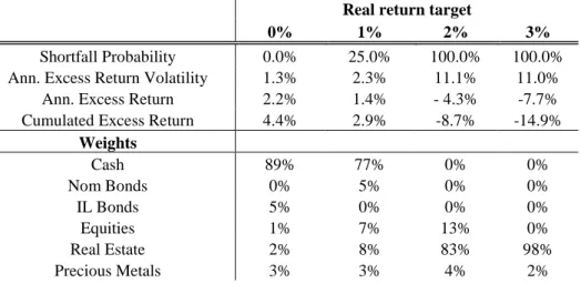
We now consider the consequences for an investor of having a more ambitious target real return, ranging from 1% to 3%. Tables 9 to 11 and 13 to 15 in Appendix 2 present the optimal portfolio composition as well as the descriptive statistics of the minimum shortfall probability portfolios,12 for the first and second sample periods.

12

(21)

Consistent with intuition, when the required real return is increased, the shortfall probability increases strongly in both sub-periods. In the first period, for a 2Y horizon investor, the minimum shortfall probability is 11.7% for a target real return of 0%. It is 37.4%, 44.9% and 48.8% for a 1%, 2% and 3% real target return respectively. The results are similar for the second period: shortfall probabilities rise from 5.1% to 27.4% for a 0% to 3% real return target.

Another intuitive result is that the more the investor increases her required real return, the more the optimal portfolio composition is biased towards risky assets. Considering the first regime, for a 30-year horizon, the optimal weight of cash decreases from 69% (with a real return target of 0%) to 0% (1% to 3% target). The IL bond weight also decreases, from 11% to 0%. The explanation is intuitive: these assets provide a good inflation hedge but are not sufficient to achieve high real returns. On the contrary, the weights of risky assets (especially equities) increase. A long-term portfolio seeking to achieve inflation plus 1% should be made up of 100% equities. Of course, if the investment horizon is shorter, a larger part of the portfolio should be dedicated to cash. This finding differs significantly from a standard mean variance optimization, which always results in cash being overweighted in the portfolio, whatever the required real return. Accordingly, the shortfall probabilities of minimum variance portfolios are particularly high when the required real return is also high.

In the second sample period, the results are comparable. Increasing the real return target leads to a decrease in the cash investment and an increase in the more risky assets. A substantial portion of nominal bonds should be added to the portfolio for low required real returns. For a 30-year investor with 1% real return target, the optimal portfolio composition is 57% nominal bonds, 16% equities, 6% real estate and 20% precious metals ; while for a 3%

(22)

target it is 35% real estate and 65% precious metals. Precious metals were the most rewarding asset class during that period. This explains why, with a very ambitious real return target, the portfolio should be heavily invested in them.

To sum up, a more ambitious real return target leads to a greater shortfall probability and a different optimal portfolio composition, with a larger weight in risky assets. In an unstable and volatile economic regime, an ambitious investor should abandon IL bonds and precious metals and concentrate on equities. In a more stable economic environment, she should reduce her portfolio weight in nominal bonds and invest a higher share in real estate and especially precious metals.

Out-of-sample backtest

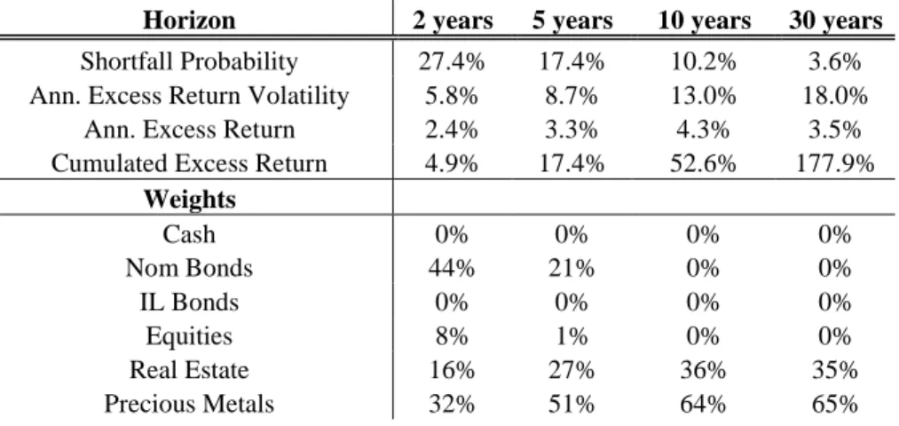
To test the robustness of our findings with an out-of-sample backtest, we perform a similar analysis on both regimes, reducing the VAR estimation period in order to backtest the ability of our optimal portfolios to hedge effectively against inflation over periods of 2 years. To test the 2-year inflation-hedging portfolios in the first regime, four optimal portfolios are estimated recursively for the periods 1973-1985, 1973-1986, 1973-1987 and 1973-1988; they are then backtested for periods of 2 years following the estimation period. The results we present (i.e. optimal weights and descriptive statistics) correspond to the mean of the four estimates. We proceed in the same way for the second regime, estimating four 2-year optimal portfolios for the periods 1991-2005, 1991-2006, 1991-2007 and 1991-2008, backtesting them on the two years after each of the periods. Tables 16 and 17 show the optimal weights of the 2-year portfolios and their out-of-sample performance for each of the regimes.

(23)

The weights of the optimised inflation-hedging portfolios estimated for the shorter periods are very similar to those presented in the previous in-sample analysis.13The portfolios constructed to hedge 2-year inflation (with a real return target of 0%) perform well, with an annualised excess return over inflation of 2.2% and 0.6% respectively for regimes 1 and 2, and a shortfall probability of zero in the first regime (the four tested portfolios were able to hedge inflation) and 25% in the second. For a 1% target real return, the optimal portfolios continue to perform well out-of-sample, with an annualised average excess return over target of 1.4% and 1.3% in the first and second regimes, respectively, and shortfall probabilities of 25% for both regimes. As soon as the target real return increases, the portfolios we construct no longer reach the target so easily, especially in the first regime, which is marked by high inflation. For a 2% target, shortfall probabilities rise to 100% in the first regime and 50% in the second. The portfolios generated mean excess returns of respectively -4.3% and -1.3%. For a 3% target real return, shortfall probabilities remain the same but the portfolios’ mean excess returns decrease to -7.7% in the first regime and -3.8% in the second. These out-of-sample findings are hardly surprising in light of our in-out-of-sample results based on 5,000 simulations. To reach high real returns, the optimal allocation assigns heavy weights to risky assets, thus generating very high shortfall probabilities, which are visible here in our out-of-sample test.

13_{Except for the high real return targets (2% and 3%) in the first regime, where the optimization leads us to}

overweight asset classes with the most attractive returns over the period. Real estate and equities compete for the first position depending on the period considered.

(24)

4. Conclusion

A key challenge for many institutional investors is the preservation of capital in real terms, while for individual investors it is building a portfolio that keeps up with the cost of living. In this paper we address the investment problem of an investor seeking to hedge inflation risk and achieve a fixed target real rate of return. The key question is thus to determine the optimal asset allocation that will preserve the investor’s capital from inflation with an acceptable probability of shortfall.

Following Campbell et al. (2003), Campbell and Viceira (2005), we used a vector-autoregressive (VAR) specification to model the joint dynamics of asset classes and state variables, and then simulated long-term holding portfolio returns for a range of different assets and inflation paths. The significant change in macroeconomic volatility and the varying nature of inflation shocks14 (leading to a change of correlation sign between inflation and the real economy) have been identified as the two main causes of the changing correlation structure between assets (Li (2002), Ilmanen (2003), Baele et al. (2009), Campbell (2009), Campbell et al. (2009)). Relying on the Goetzmann et al. (2006) test for structural change in correlation, we determined the breakpoint that best separates the sample data, ensuring the most stable correlation structure within each sub-period. We estimated a VAR model on each period and performed a simulation-based analysis. We were thus able to measure the inflation hedging properties of each asset class in each regime and determine the allocation that

14_{The 1970’s and 1980’s were marked by strong supply shocks (especially oil shocks in 1973 and 1979) which}

accounted for more than 80% of the inflation volatility and dominated the contribution of demand shocks in the economy. The 80’s and 90’s have seen a reduction in the amplitude of both supply and demand shocks. If the contribution of demand shocks dominate during that regime, the reduced volatility of the demand side of the economy (government spending, residential housing and inventory changes) has been an important source of improved stability (Gordon (2005)).

(25)

maximises above-target returns (inflation + x%) with the constraint that the shortfall probability remains below a threshold set by the investor.

Our results confirm that the presence of macroeconomic regimes radically alters the investor’s optimal allocation. In a volatile regime marked by countercyclical inflation, a safety-first investor having a pure inflation target should be mainly invested in cash when her investment horizon is short and should increase her allocation to IL bonds and precious metals when horizon increases. In a more stable economic environment with procyclical inflation shocks, the optimal investment set changes radically. Mainly invested in cash when investment horizon is short, an investor should increase her investment in nominal bonds, but also, to a lesser extent, to precious metals and real estate when her horizon increases. Our results confirm the value of alternative asset classes in protecting the portfolio against inflation.

Having a more ambitious real return target (from 1% to 3%) leads automatically to a greater shortfall probability, but also to a different optimal portfolio composition. Cash does not provide sufficient returns to achieve the positive real rate target. A larger weight should be dedicated to risky assets, which make it possible to achieve higher returns (with a greater shortfall probability). In the first period, an ambitious investor should gradually abandon IL bonds and precious metals and concentrate on equities. In the second period, she should reduce her portfolio weight in nominal bonds and invest a higher share in real estate and especially precious metals.

In the real world, many investors (especially pension funds) do not operate with a single well-defined goal but rather have to cope with multiple and sometimes contradictory

(26)

objectives, with long-term return shortfall probability constraints and short term performance objectives. An interesting development of this work would be to take these different constraints into account. Structural breaks and regime shifts are an important issue for an investor. In this paper we have described how the two main regimes that have affected the economy since the 1970s may have influenced the relationship between inflation and asset prices. We have also shown how they have radically altered the optimal allocation of an investor seeking to hedge inflation risk. The question now is to determine what regime lies ahead. While the recent resurgence of higher macroeconomic volatility might suggest a gradual move away from the “Great Moderation”, there is no certainty that the forthcoming regime will be similar to the one in the 1970s and 1980s. The four decades under study are unfortunately not that long, and the inflationary episodes experienced in the 1970s may not necessarily be representative of future inflation shocks in developed economies. The possibility of different future relationships cannot be ruled out.

(27)

References

Agarwal, V., Naik, N., 2004. Risks and Portfolio Decisions Involving Hedge Funds. Review of Financial Studies, 17(1), 63–8.

Amenc, N., Martellini, L., Ziemann, V., 2009. Alternative Investments for Institutional Investors, Risk Budgeting Techniques in Asset Management and Asset-Liability Management. The Journal of Portfolio Management, 35(4), 94-110.

Amisano, G., Giannini, C., 1997. Topics in structural VAR econometrics, Second edition, Berlin and New York: Springer.

Attié, A.P., Roache, S.K., 2009. Inflation Hedging for Long-Term Investors. IMF Working Paper, No. 09-90, April.

Baele, L., Bekaert ,G., Inghelbrecht, K., 2009. The Determinants of Stock and Bond Return Comovements. NBER Working Paper, No. 15260, August.

Balduzzi, P., Lynch, A.W., 1999. Transaction Costs and Predictability: Some Utility Cost Calculations. Journal of Financial Economics, 52, 47-78.

Barberis, N., 2000. Investing for the Long Run when Returns are Predictable. The Journal of Finance, 40(1), 225-264.

(28)

Barnett, W., Chauvet, M., 2008. The End of Great Moderation?. University of Munich, Working Paper.

Bekaert, G., Engstrom, E., 2009. Inflation and the Stock Market: Understanding the Fed Model. NBER Working Paper, No. 15024, June.

Berardi, A., 2005. Real Rates, Excepted Inflation and Inflation Risk Premia Implicit in Nominal Bond Yields. Università di Verona Working Paper, October.

Bernanke, B., 2004. The Great Moderation. Remarks at the meetings of the Eastern Economic Association, Washington, DC, February.

Billio, M., Casarin, R., 2007. Stochastic Optimization for Allocation Problems with Shortfall Constraints, Applied Stochastic Models in Business and Industry, 23(3), 247-271.

van Binsbergen, J.H., Brandt, M.W., 2007. Optimal Asset Allocation in Asset Liability Management. NBER Working Paper, No.12970.

Blanchard, O. J., Simon, J.A., 2001. The Long and Large Decline in US Output Volatility. Brookings Papers on Economic Activity, 2001(1), 135-164.

Brandt, M.W., 1999. Estimating Portfolio and Consumption Choice: A Conditional Euler Equations Approach. The Journal of Finance, 54(5), 1609-1645.

(29)

Brandt, M.W., Wang, K.Q., 2003. Time-Varying Risk Aversion and Unexpected Inflation. Journal of Monetary Economics, 50(7), 1457-1498.

Brennan, M., Schwartz, E., Lagnado, R., 1997. Strategic Asset Allocation. Journal of Economic Dynamics and Control, 21, 1377-1403.

Brière, M., Signori, O., 2009. Do Inflation-Linked Bonds still Diversify?. European Financial Management, 15 (2), 279-339.

Brière M., Signori O., Burgues A., 2010. Volatility Exposure for Strategic Asset Allocation. The Journal of Portfolio Management, 36(3), 105-116.

Campbell, J.Y., 2009. The Changing Role of Nominal Bonds in Asset Allocation, The Geneva Risk and Insurance Review, 34, 89-104.

Campbell, J.Y., Ammer, J., 1993. What Moves the Stock and Bond Markets: A Variance Decomposition for Long-Term Asset Returns. The Journal of Finance, 48(1), 3-37.

Campbell, J.Y., Chan, Y.L., Viceira, L.M., 2003. A Multivariate Model for Strategic Asset Allocation. Journal of Financial Economics, 67, 41-80.

Campbell, R., Huisman, R., Koedijk, K., 2001. Optimal Portfolio Selection in a Value-at-Risk Framework. Journal of Banking and Finance, 25, 1789-1804.

(30)

Campbell, J.Y., Shiller, R., 1988. Stock Prices, Earnings and Expected Dividends. The Journal of Finance, 43(3), 661-676.

Campbell, J.Y., Sunderam A., Viceira L.M., 2009. Inflation Bets or Deflation Hedge? The Changing Risk of Nominal Bonds, NBER Working Paper, No. 14701, January.

Campbell, J.Y., Viceira, L.M., 2002. Strategic Asset Allocation: Portfolio Choice for Long Term Investors. Oxford University Press, Oxford.

Campbell, J.Y., Viceira, L.M., 2005. The Term Structure of the Risk-Return Tradeoff. Financial Analyst Journal, 61, 34-44.

Campbell, J.Y., Vuolteenaho, T., 2004. Inflation Illusion and Stock Prices. NBER Working Paper, No. 10263, February.

Campbell, J.Y., Yogo, M., 2006. Efficient Tests of Stock Return Predictability. Journal of Financial Economics, 81, 27-60.

Cochrane, J.H., 2009. Understanding Fiscal and Monetary Policy un 2008-2009. University of Chicago Working Paper, October.

D’Amico, S., Kim, D., Wei, M., 2008. Tips from TIPS: the informational content of Treasury Inflation-Protected Security prices. BIS Working Paper, No. 248, March.

(31)

Eijffinger, S.C.W., Geraats, P.M., van der Cruijsen, C.A.B., 2006. Does Central Bank Transparency Reduce Interest Rates?. CEPR Working Paper, No. 5526, March.

Fugazza, C., Guidolin, M., Nicodano, G., 2007. Investing in the Long-Run in European Real Estate. Journal of Real Estate Finance and Economics, 34, 35-80.

Geske, R., Roll, R., 1983. The Fiscal and Monetary Linkage Between Stock Returns and Inflation. The Journal of Finance, 38(1), 1-33.

Goetzmann, W.N., Li, L., Rouwenhorst, K.G., 2005. Long-term global market correlations. Journal of Business, 78(1), 1-38.

Goetzmann, W.N., Valaitis, E., 2006. Simulating Real Estate in the Investment Portfolio: Model Uncertainty and Inflation Hedging. Yale ICF Working Paper, No. 06-04 , March.

Gordon, R.J., 2005. What Caused the Decline in US Business Cycle Volatility?. NBER Working Paper No. 11777, November.

Guidolin, M., Timmermann, A., 2005. Strategic Asset Allocation and Consumption Decisions under Multivariate Regime Switching. Federal Reserve Bank of Saint Louis Working Paper, No. 2005-002.

Harlow, W.V., 1991. Asset Pricing in a Downside-Risk Framework. Financial Analyst Journal, 47(5), 28-40.

(32)

Hoevenaars, R.R., Molenaar, R., Schotman, P., Steenkamp, T., 2008. Strategic Asset Allocation with Liabilities: Beyond Stocks and Bonds. Journal of Economic Dynamic and Control, 32, 2939-2970.

Hsieh, C.T., Hamwi, I.S., Hudson, T., 2002. An Inflation-Hedging Portfolio Selection Model. International Advances in Economic Research, 8(1), 20-34.

Ilmanen, A., 2003. Stock-Bond Correlations. The Journal of Fixed Income, 13(2), 55-66.

Kandel, S., Stambaugh, R., 1996. On the Predictability of Stock Returns: an Asset Allocation Perspective. The Journal of Finance, 51(2), 385-424.

Kim, D.H., Wright, J.H., 2005. An Arbitrage-Free Three-Factor Term Structure Model and the Recent Behavior of Long-Term Yields and Distant-Horizon Forward Rates. Board of the Federal Reserve Research Paper Series, No. 2005-33, August.

Kizys, R., Spencer, P., 2008. Assessing the Relation between Equity Risk Premium and Macroeconomic Volatilities in the UK. Quantitative and Qualitative Analysis in Social Sciences, 2(1), 50-77.

Kothari, S., Shanken, J., 2004. Asset Allocation with Inflation-Protected Bonds. Financial Analyst Journal, 60(1), 54-70.

Leibowitz, M.L., 1987. Pension Asset Allocation through Surplus Management. Financial Analyst Journal, 43(2), 29-40.

(33)

Leibowitz, M.L., Henriksson, R.D., 1989. Portfolio Optimisation with Shortfall Constraints: a Confidence-Limit Approach to Managing Downside Risk. Financial Analyst Journal, 45(2), 34-41.

Leibowitz, M.L., Kogelman, S., 1991. Asset Allocation under Shortfall Constraints. The Journal of Portfolio Management, 17(2), 18-23.

Lettau, M., Ludvigson, S. C., Wachter, J. A., 2009. The Declining Equity Premium: What Role Does Macroeconomic Risk Play?. Review of Financial Studies, Oxford University Press for Society for Financial Studies, 21(4), 1653-1687.

Li, L., 2002. Macroeconomic Factors and the Correlation of Stock and Bond Returns. Yale ICF Working Paper, No. 02-46.

Lucas, A., Klaassen, P., 1998. Extreme Returns, Downside Risk and Optimal Asset Allocation. The Journal of Portfolio Management, 25(1), 71-79.

Lynch, A., 2001. Portfolio Choice and Equity Characteristics: Characterizing the Hedging Demands Induced by Return Predictability. Journal of Financial Economics, 62, 67-130.

Modigliani, F., Cohn, R., 1979. Inflation, Rational Valuation and the Market. Financial Analyst Journal, 35(2), 24-44.

(34)

Okunev J., Wilson P. and Zurbruegg R., 2000. The Causal Relationship between Real Estate and Stock Markets, The Journal of Real Estate Finance and Economics, 21(3), 251-261.

Ritter, J., Warr, R.S., 2002. The Decline of Inflation and the Bull Market of 1982-1999. Journal of Financial and Quantitative Analysis, 37(1), 29-61.

Roy, A.D., 1952. Safety First and the Holding of Assets. Econometrica, 20(3), 431-449.

Sharpe, W.F., Tint, L.G., 1990. Liabilities: a New Approach. The Journal of Portfolio Management, Winter, 16(2), 5-10.

Smith, G., Gould, D.P., 2007. Measuring and Controlling Shortfall Risk in Retirement. The Journal of Investing, Spring, 16(1), 82-95.

Summers, P. M., 2005. What caused The Great Moderation? Some Cross-Country Evidence. Economic Review Federal Reserve Bank of Kansas City, 90(3), 5-32.

Walsh, C., 2009. Using Monetary Policy to Stabilize Economic Activity. University of California San Diego Working Paper, August.

(35)

Appendix 1

Table 1: Summary statistics of monthly returns, January 1973-December 2010

Cash

Nom

Bonds IL bonds Equities

Real Estate Precious Metals Ann. Ret. 5.6% 7.8% 6.5% 9.2% 9.0% 7.7% Max Monthly 1.3% 11.3% 13.9% 16.4% 26.9% 36.9% Min Monthly 0.0% -9.0% -13.8% -23.9% -36.4% -34.6% Ann. Vol. 0.9% 7.6% 9.8% 15.9% 18.6% 22.3% Risk/Adjusted Ret.* 6.1 1.0 0.7 0.6 0.5 0.3 Skewness 0.6 0.2 0.1 -0.7 -1.2 0.4 Kurtosis 3.7 5.8 6.9 5.5 11.8 8.9

(36)

Table 2: Results of VAR model, parameter estimates, January 1973-December 1990 Cash Nom Bonds IL Bonds Equities Real Estate Precious Metals Inflation Div. Yield Term Spread Cash(-1) 0.96 0.76 -1.30 -1.68 -3.24 -3.73 0.10 1.62 54.88 ( 48.69) ( 0.74) (-1.16) (-0.86) (-1.65) (-1.12) ( 0.55) ( 1.22) ( 2.62) Nom Bonds(-1) -0.01 0.16 1.01 0.01 0.45 -0.14 -0.04 -0.20 2.17 (-6.25) ( 1.57) ( 9.39) ( 0.07) ( 2.35) (-0.42) (-2.20) (-1.52) ( 1.07) IL Bonds(-1) 0.00 -0.08 -0.17 0.22 0.09 0.42 0.01 0.00 3.51 (-0.56) (-1.06) (-2.06) ( 1.58) ( 0.64) ( 1.77) ( 1.01) ( 0.03) ( 2.32) Equities(-1) 0.00 -0.02 -0.07 -0.13 0.02 -0.10 0.00 -0.36 -0.93 ( 1.55) (-0.48) (-1.28) (-1.48) ( 0.20) (-0.64) ( 0.53) (-5.92) (-0.98) Real Estate(-1) 0.00 -0.06 -0.06 0.15 -0.07 0.24 -0.01 -0.08 -1.15 ( 1.52) (-1.19) (-1.28) ( 1.73) (-0.76) ( 1.60) (-1.15) (-1.35) (-1.21) Precious Metals(-1) 0.00 -0.07 -0.06 -0.02 0.00 0.06 0.00 -0.01 -0.59 ( 2.36) (-3.04) (-2.50) (-0.36) (-0.07) ( 0.82) ( 1.32) (-0.31) (-1.33) Inflation(-1) 0.00 -0.17 0.12 -0.22 -0.19 0.22 1.00 0.14 0.00 ( 0.64) (-2.51) ( 1.64) (-1.72) (-1.46) ( 1.00) ( 87.85) ( 1.63) (-0.00) Div. Yield(-1) 0.00 0.02 0.02 0.06 0.09 -0.01 0.00 0.96 -0.17 (-0.28) ( 2.14) ( 1.28) ( 2.68) ( 4.31) (-0.30) (-2.50) ( 66.8) (-0.74) TermSpread(-1) 0.00 0.00 0.00 0.00 0.00 0.00 0.00 0.00 0.27 (-3.75) ( 1.50) ( 0.71) (-0.24) (-0.46) (-0.22) (-1.20) (-0.91) ( 4.07) Adj. R2/F.stat 0.95 0.09 0.41 0.06 0.13 0.03 0.98 0.98 0.16 (452.00) (3.45) (17.15) (2.62) (4.68) (1.70) (1446.24) (941.59) (5.36)

t-stat are given in parenthesis. The last row reports the adjusted-R2 and the F-statistics of joint significance.

Table 3: VAR residuals, correlation coefficients, January 1973-December 1990

Cash

Nom

Bonds IL Bonds Equities

Real Estate

Precious

Metals Inflation Div. Yield Term Spread

Cash 1.00 Nom Bonds -0.36 1.00 IL Bonds -0.46 0.84 1.00 Equities -0.16 0.27 0.22 1.00 Real Estate -0.28 0.20 0.16 0.62 1.00 Precious Metals -0.18 -0.04 0.00 0.03 0.09 1.00 Inflation 0.04 -0.09 -0.02 -0.15 -0.09 0.26 1.00 Div. Yield 0.14 -0.22 -0.26 -0.80 -0.55 0.01 0.20 1.00 Term Spread -0.85 -0.10 -0.06 0.02 0.20 0.21 0.01 0.02 1.00

(37)

Table 4: Results of VAR model, parameter estimates, January 1991-December 2010

Cash

Nom

Real Estate

Precious

Metals Inflation Div. Yield

Term Spread Cash(-1) 1.00 1.28 1.10 5.89 -0.16 -3.12 0.27 -2.87 0.64 ( 134.64) ( 1.50) ( 1.15) ( 2.80) (-0.06) (-1.47) ( 1.39) (-2.01) ( 0.05) Nom Bonds(-1) 0.00 0.13 0.61 0.07 0.51 0.09 -0.05 -0.25 -5.81 (-3.86) ( 1.43) ( 6.06) ( 0.29) ( 1.84) ( 0.41) (-2.41) (-1.65) (-5.07) IL Bonds(-1) 0.00 -0.06 -0.22 0.13 0.38 -0.17 0.03 -0.14 4.13 (-2.87) (-0.73) (-2.47) ( 0.67) ( 1.51) (-0.85) ( 1.55) (-1.00) ( 3.98) Equities(-1) 0.00 -0.08 0.00 -0.01 0.33 0.02 0.00 -0.48 -0.55 ( 2.04) (-2.40) ( 0.07) (-0.12) ( 3.31) ( 0.19) ( 0.69) (-8.86) (-1.34) Real Estate(-1) 0.00 -0.04 -0.02 0.05 0.00 -0.05 0.01 -0.02 0.43 ( 0.02) (-1.69) (-0.81) ( 0.81) ( 0.06) (-0.82) ( 1.19) (-0.57) ( 1.33) Precious Metals(-1) 0.00 -0.02 -0.04 -0.04 -0.13 -0.16 0.02 0.05 0.29 ( 0.22) (-0.86) (-1.35) (-0.54) (-1.57) (-2.33) ( 3.54) ( 1.15) ( 0.84) Inflation(-1) 0.00 0.01 -0.10 -0.93 -0.38 -0.51 0.92 0.88 0.79 (-1.02) ( 0.10) (-0.84) (-3.45) (-1.13) (-1.88) ( 37.58) ( 4.82) ( 0.56) Div. Yield(-1) 0.00 0.00 0.00 0.02 0.00 0.00 0.00 0.98 0.02 (-0.18) ( 0.75) ( 0.30) ( 2.33) ( 0.08) (-0.28) (-1.57) ( 155.) ( 0.36) TermSpread(-1) 0.00 0.00 -0.01 0.01 0.03 -0.01 0.00 -0.02 0.33 (-5.99) ( 0.40) (-1.12) ( 1.07) ( 2.00) (-0.97) (-0.23) (-2.35) ( 4.63) Adj. R2/F.stat 0.99 0.08 0.16 0.04 0.09 0.04 0.89 0.99 0.18 (2725.44) (3.35) (6.22) (2.20) (3.77) (1.99) (212.79) (2841.17) (6.68)

t-stat are given in parenthesis. The last row reports the adjusted- R2 and the F-statistics of joint significance.

Table 5: VAR residuals, correlation coefficients, January 1991-December 2010

Cash

Nom

Real Estate

Precious

Metals Inflation Div. Yield Term Spread

Cash 1.00 Nom Bonds -0.19 1.00 IL Bonds -0.22 0.74 1.00 Equities 0.09 -0.09 0.03 1.00 Real Estate 0.11 0.06 0.14 0.57 1.00 Precious Metals -0.01 0.12 0.25 0.01 0.14 1.00 Inflation 0.08 -0.10 0.07 0.07 0.11 0.16 1.00 Div. Yield -0.18 0.12 -0.03 -0.73 -0.42 -0.10 -0.05 1.00 Term Spread -0.61 -0.50 -0.46 -0.02 -0.20 -0.11 -0.04 0.07 1.00

(38)

Table 6: Probabilities of not achieving the inflation target for individual assets, January 1973-December 1990

Horizon 2 years 5 years 10 years 30 years

Cash 17% 21% 18% 9% Nom Bonds 38% 34% 30% 20% IL Bonds 48% 43% 39% 29% Equities 38% 29% 21% 7% Real Estate 45% 41% 34% 22% Precious Metals 48% 47% 47% 46%

Table 7: Probabilities of not achieving the inflation target for individual assets, January 1991-December 2010

Cash 22% 34% 47% 69% Nom Bonds 16% 6% 3% 0% IL Bonds 29% 22% 18% 14% Equities 31% 31% 33% 33% Real Estate 29% 22% 15% 4% Precious Metals 25% 11% 5% 0%

(39)

Figure 1 : Correlations between asset returns and inflation depending on the investment horizon, January 1973 – December 1990

Figure 2 : Correlations between asset returns and inflation depending on the investment horizon, January 1991– December 2010

-1 -0.8 -0.6 -0.4 -0.2 0 0.2 0.4 0.6 0.8 0 60 120 180 240 300 360 Months C o rr e la tio n C o e ff ic ie n t Cash Nom Bonds IL Bonds Equities Real Estate Precious metals -1 -0.8 -0.6 -0.4 -0.2 0 0.2 0.4 0.6 0.8 1 0 60 120 180 240 300 360 Months C o rr e la tio n C o e ff ic ie n t _Cash Nom Bonds IL Bonds Equities Real Estate Precious metals

(40)

Appendix 2

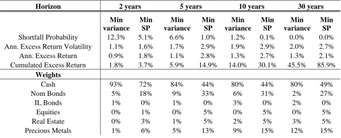
Table 8: Minimum variance and minimum shortfall probability portfolios, real return target 0%, January 1973-December 1990

*SP designs Shortfall Probability

**Excess returns are measured over target.

Table 9: Minimum shortfall probability portfolio, real return target 1%, January 1973- December 1990

Shortfall Probability 37.4% 34.1% 27.3% 13.7%

Ann. Excess Return Volatility 2.3% 8.7% 16.0% 16.0%

Ann. Excess Return 0.5% 1.5% 2.7% 2.3%

Cumulated Excess Return 1.0% 8.0% 30.6% 95.8%

Weights Cash 86% 46% 0% 0% Nom Bonds 3% 0% 0% 0% IL Bonds 0% 0% 0% 0% Equities 8% 50% 97% 99% Real Estate 0% 0% 0% 0% Precious Metals 2% 5% 3% 1%

Min variance Min SP* Min variance Min SP Min variance Min SP Min variance Min SP Shortfall Probability 13.0% 11.7% 15.4% 15.4% 13.1% 12.5% 4.4% 3.1%

Ann. Excess Return Volatility 1.6% 1.6% 2.8% 3.0% 3.6% 4.1% 4.0% 5.0%

Ann. Excess Return** 1.3% 1.3% 1.2% 1.3% 1.2% 1.4% 1.1% 1.4%

Cumulated Excess Return 2.6% 2.6% 6.4% 6.7% 12.8% 14.9% 38.1% 51.1%

Weights Cash 92% 92% 87% 87% 82% 79% 77% 69% Nom Bonds 0% 0% 0% 0% 0% 0% 0% 0% IL Bonds 6% 5% 8% 5% 12% 8% 16% 11% Equities 0% 0% 0% 2% 0% 7% 0% 14% Real Estate 0% 0% 0% 0% 0% 0% 0% 0% Precious Metals 2% 2% 5% 5% 6% 6% 7% 7%

(41)

Table 10: Minimum shortfall probability portfolio, real return target 2%, January 1973-December 1990

Ann. Excess Return 1.3% 1.8% 1.9% 1.4%

Cumulated Excess Return 2.7% 9.4% 20.3% 51.0%

Table 11: Minimum shortfall probability portfolio, real return target 3%, January 1973-December 1990

Ann. Excess Return 0.3% 0.8% 1.9% -0.4%

Cumulated Excess Return 0.7% 3.8% 20.3% -10.6%

Table 12: Minimum variance and minimum shortfall probability portfolios, real return target 0%, January 1991- December 2010

Min variance Min SP Min variance Min SP Min variance Min SP Min variance Min SP Shortfall Probability 12.3% 5.1% 6.6% 1.0% 1.2% 0.1% 0.0% 0.0%

Ann. Excess Return Volatility 1.1% 1.6% 1.7% 2.9% 1.9% 2.9% 2.0% 2.7%

Ann. Excess Return 0.9% 1.8% 1.1% 2.8% 1.3% 2.7% 1.3% 2.1%

Cumulated Excess Return 1.8% 3.7% 5.9% 14.9% 14.0% 30.1% 45.5% 85.9%

Weights Cash 93% 72% 84% 44% 80% 44% 80% 49% Nom Bonds 5% 18% 9% 33% 6% 31% 2% 27% IL Bonds 1% 0% 1% 0% 3% 0% 2% 0% Equities 0% 1% 0% 5% 0% 5% 0% 5% Real Estate 0% 3% 1% 5% 2% 5% 3% 5% Precious Metals 1% 6% 5% 13% 9% 15% 12% 15%