HAL Id: hal-02377276
https://hal.archives-ouvertes.fr/hal-02377276
Submitted on 23 Nov 2019
HAL is a multi-disciplinary open access archive for the deposit and dissemination of sci-entific research documents, whether they are pub-lished or not. The documents may come from teaching and research institutions in France or abroad, or from public or private research centers.
L’archive ouverte pluridisciplinaire HAL, est destinée au dépôt et à la diffusion de documents scientifiques de niveau recherche, publiés ou non, émanant des établissements d’enseignement et de recherche français ou étrangers, des laboratoires publics ou privés.
Toward direct, micron-scale XRF elemental maps and
quantitative profiles of wet marine sediments
Philippe Boning, Jérôme Rose, Edouard Bard
To cite this version:
Philippe Boning, Jérôme Rose, Edouard Bard. Toward direct, micron-scale XRF elemental maps and quantitative profiles of wet marine sediments. Geochemistry, Geophysics, Geosystems, AGU and the Geochemical Society, 2007, �10.1029/2006GC001480�. �hal-02377276�
Toward direct, micron-scale XRF elemental maps and quantitative
profiles of wet marine sediments
Philipp Böning, Edouard Bard, and Jérôme Rose
CEREGE - Collège de France, UMR6635 CNRS, University Paul Ce´zanne Aix-Marseille III, Europoˆle de l’Arbois, BP80, F-13545 Aix-en-Provence Cedex 4, France (philipp@cerege.fr)
[1] Here we describe a chemical analysis technique for Ca, Fe, K, Sr, Ti, and S using a recently developed Micro-XRF analyzer (Micro-XRF) with a 100-mm resolution and an XRF whole-core scanner (XRF-S) with a 5-mm resolution for selected sediment sections from a continental margin sediment core. The Micro-XRF produces highly resolved element maps of individual sections, and the calculation of individual continuous element profiles is based on overlap measurements of successive sections. By means of discrete subsamples analyzed by ICP-OES, the two XRF data sets are successfully calibrated to provide quantitative profiles of Ca, Fe, K, Sr, and Ti. We discuss the advantages and limitations of both XRF techniques. A comparison of the two independent XRF data sets demonstrates the overall high consistency and accuracy of both techniques. The resulting element profiles and detailed XRF maps clearly show that the Micro-XRF is a powerful tool for studying at high resolution the chemical transitions linked to paleoenvironmental changes. For example, the discrimination between provenance changes and diagenetical effects on the Fe profile can be achieved by the combined inspection of the Fe/Ti profile and S maps. This highlights the usefulness of the XRF maps for clarification of profile ambiguities and clearly distinguishes the Micro-XRF from other technical devices producing elemental profiles only.
Components: 7356 words, 8 figures, 3 tables.
Keywords: Micro-XRF scanner; high-resolution XRF analysis; major and trace elements.
1. Introduction
[2] Over the last few years, significant progress has been made in the field of high-resolution analysis of natural samples based on X-ray imaging techniques (absorption, micro-fluorescence, transmission and tomography). Micro X-Ray Fluorescence Analysis (Micro-XRF) is one of the techniques that has been developed very rapidly, mainly by means of
synchrotron radiation and X-ray focusing devices. Since it is non-destructive and able to map samples on a micrometer (mm) scale, Micro-XRF is nowadays a well-established analytical method over a wide range of fields of application, such as materials science, archaeometry, life sciences and, as shown here, geochemical studies.
[3] High-resolution studies on continuous sedimentary archives are much in demand for the understanding of high-frequency climate change on a seasonal to millennial scale.
Consequently, it is necessary to look at individual chemical and structural phase transitions in closer detail, which offers the possibility of linking geochemistry, sedimentology and
mineralogy in combined studies. This important issue can be addressed using MicroXRF, whose resolution is better than the millimeter scale.
[4] We present data on calcium (Ca), iron (Fe), strontium (Sr), potassium (K) and titanium (Ti), which are important constituents of marine sediments commonly used as tracers for paleoenvironmental reconstructions. Biogenic Ca and Sr typically indicate the presence of calcareous organisms (made of calcite or aragonite), whereas the other elements usually indicate the presence of lithogenic material or diagenetical sulphides (Fe). Elemental XRF scanners, with a resolution of several mm, are commonly used to detect these and other elements in sediments from various ancient and recent marine environments [e.g., Peterson et al., 2000; Ro¨hl and Abrams, 2000]. By contrast, only few published XRF data are available for wet marine sediments on a sub-millimeter scale [von Rad et al., 2002; Haug et al., 2003; Kido et al., 2006].
[5] In this paper, we present (1) a technique using the XGT 5000 Micro-XRF analyzer recently developed by Horiba-Jobin-Yvon, (2) elemental data (Ca, Fe, K, Sr and Ti) from partly
laminated continental margin sediments acquired with Micro-XRF and a routinely used whole-core XRF Scanner (abbreviated here as XRF-S), (3) the successful calibration of both XRF data sets to element contents derived from ICP-OES, (4) a cross-check of both quantified Micro-XRF and XRF-S data, and (5) a promising outlook on the application of Micro-XRF to paleo-environmental studies.
2. Materials and Methods
2.1. Sample Selection Strategy
[6] The material for this study stems from core MD04-2876 ($25 m length) retrieved during cruise MD 143 CHAMAK of the Marion Dufresne in September/October 2004. The working half of the core was sampled with u-channels. The sediments of this specific core are made up of clays with varying amounts of CaCO 3 (min. 5 to max. 40 wt%). In the laboratory, the u-channels were analyzed using the Avaatech 1 XRF whole-core scanner. Then, 67 samples were taken from the entire core for chemical analysis by ICP-OES. For the subsequent Micro-XRF analysis (XGT 5000
Horiba Jobin-Yvon), we selected two independent sections (40 cm each), one from the upper and one from the lower half of the core. The first section represents a transition from dark, laminated and carbonate-bearing to light, non-laminated and carbonate-rich sediments (called Section 1), whereas the second section represents dark laminated and carbonate-bearing sediments with varying degrees of lamination preservation (called Section 2). A total of 39 samples were taken from both sections for Micro-XRF data calibration. For further technical details, see below.
2.2. XRF Core Scanner
[7] The XRF-S (Avaatech 1 XRF whole-core scanner at the University of Bremen) is a non-destructive routine analysis system for scanning the surface of sediment cores or u-channels [Jansen et al., 1998; Ro¨hl and Abrams, 2000]. The XRF-S is equipped with a Molybdenum
X-ray source (3–50 kV), a Si(Li) Peltier-cooled PSI energy-dispersive X-X-ray (EDX) spectrometer (Kevex TM ) with a 125-mm beryllium window and a multichannel analyzer. This system configuration allows the analysis of elements from Al (atomic no. 13) to Ba (atomic no. 56).
[8] Prior to daily analysis, the instrument was calibrated against a set of pressed powder standards [Jansen et al., 1998]. The sediment surface was lightly scraped with a microscope slide (parallel to lamination) to obtain a clean, smooth and flat surface. After that, the sediment surface was covered with Ultralene 1 X-ray transmission foil to avoid desiccation. Over the entire core, we analyzed statistically significant element intensities of Ca, Fe, K and Ti at 0.5-cm intervals, each measurement covering an area of 0.4 cm 2 (0.4 cm long  1 cm wide), using a 30-s count time, 10 kV X-ray voltage and a current of 0.6 mA. The X-ray spot size was obtained using lateral slits. Acquired XRF spectra were processed with the Kevex 2 software Toolbox # (including successive application of background subtraction, sum-peak and escape-peak correction, deconvolution and peak integration [Ro¨hl and Abrams, 2000]). The resulting data are expressed as element intensities in counts per second (cps).
Heterogeneities due to variable water content, porosity, grain-size differences and rough surfaces lead to scattering and bias in the scanner data which is commonly of the order of $200 cps at the 2000 cps level [Jansen et al., 1998].
2.3. Micro XRF Analyzer
[9] The XGT-5000 X-ray Analysis Microscope (Horiba-Jobin-Yvon), here referred to as Micro-XRF, was designed to measure and analyze simultaneously the X-ray spectrum, the
transmitted X-ray image and the fluorescent X-ray image (or map) of a sample. The Micro-XRF is a non-destructive analysis system for high-resolution scanning of hard or soft sample surfaces [e.g., Rose et al., 2006]. The highly focused and intense X-ray beam is generated with a Rhodium X-ray tube (15–50 kV) using a current adjustable up to 1 mA and focused with X-ray guide tubes, whose inner diameter is either 100 or 10 mm (Figure 1) [Hosokawa et al., 1997]. X-ray emission from the irradiated sample is detected with an energy-dispersive X-ray (EDX) spectrometer equipped with a liquid-nitrogencooled high-purity Si detector. The system configuration allows the analysis of elements from Na (atomic no. 11) to U (atomic no. 92). An X-ray tube voltage of 50 kV is applied with a current of 1.0 mA and an X-ray radiation diameter of 100 mm for the determination of Ca, Fe, K, Sr and Ti by using their Ka line intensities.
Figure 1. Schematic view of the measuring chamber of the XGT-5000 Micro-XRF Analyzer (Horiba–JobinYvon) at CEREGE. The incident beam hits the sample surface perpendicularly, while the detector makes an angle of 45°with the sample surface. Image not to scale.
[10] The analysis probe chamber of the XGT-5000 (X-ray source and detector) is under vacuum (Figure 1), which increases sensitivity for light elements. However, samples are analyzed under the probe in the xy direction at normal atmospheric pressure. A constant distance of 1 mm is maintained between the analysis probe chamber and the sediment surface to minimize absorption effects by the air between the probe and the sample.
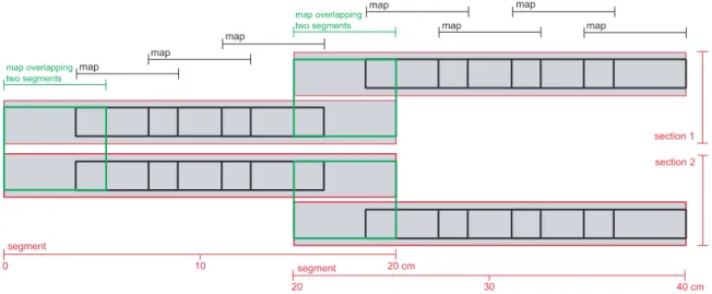
[11] Prior to analysis, the u-channels in the studied core were carefully cut into 20 cm segments to fit the relatively small analysis chamber (Figure 2). Care was taken not to loose or squeeze out sediment at the margins of each segment, so as to avoid disturbing the sedimentary continuity. The sediment surface was covered with a PVC thin film (Ecopla 1 , 10 mm thick) to avoid desiccation. Each segment was stored in a gas-tight plastic box and kept cool at 4°C.
[12] First, an element map of 5.12 Â 5.12 cm (26.2 cm 2 ) was produced covering two segments (called the reference overlap; shown as a green rectangle on the left in Figure 2). Then, for each segment, a map of 5.12 cm x 1.28 cm (6.55 cm 2 ) was constructed, which overlapped the reference by a length of about 1.2 cm and a maximum width of 1.28 cm ($1.54 cm 2 ). Consequently, further maps of 6.55 cm 2 were produced that overlapped each other by $1.54 cm 2 .
Figure 2.Diagram showing the measuring protocol of the Micro-XRF on the two 40 cm sediment sections.
Figure 3. Example of the data processing described in the text. (a) Two successive maps with corresponding elemental profiles. The area of the overlap is indicated by the dashed
rectangle. (b) Scatterplot of the data from the two overlapping maps: gsv, grayscale values.
[13] For optimum counting, the measuring time was 15 ms per pixel (i.e., 0.1 Â 0.1 mm, i.e., one data point) repeated at least 25 times resulting in a measuring time of $7 h per 6.55 cm 2 . For each pixel in the XRF map the software first deconvolved the measured XRF spectrum to element counts, which were then auto-converted to grayscale values using a linear interpolation. Each data point along the downcore profile (along the x axis) is the average value of a maximum of 128 pixels (map width or y direction) resulting in element profiles with 512 data points (map length or x direction). For each point on the x axis representing 100 mm, the counting time was therefore at least 34 s. Obvious cracks and holes were discarded for element profile calculation.
[14] To obtain an element profile for the entire segment of 20 cm, the individual profiles had to be fitted to the profile from the reference overlap. This resulted in scatterplots with a linear regression (according to the equation y = a . x + b). For elements such as Fe, Ca, and Sr,
the squared correlation coefficient r 2 is high and significant, ranging between 0.72 and 0.95 (a representative segment is shown in Figures 3a and 3b). The linear equation was then used to rescale the profiles and element maps in order to make them fully compatible. In effect, the slope a and intercept b allow us to correct for slight changes of the sensitivity and baseline between different scans of the Micro-XRF instrument.
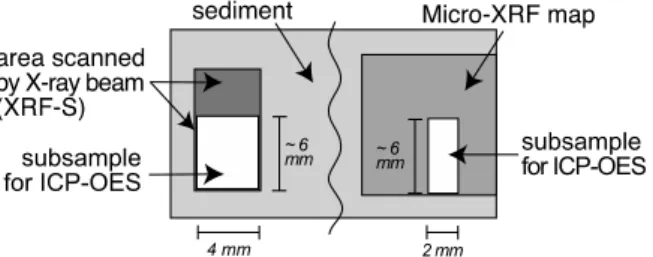
Figure 4. Sketch showing subsamples taken for the quantification of XRF-S and Micro-XRF data using ICP-OES.
[15] For K and Ti, however, a larger scatter was obtained for overlapping profiles, which resulted in smaller r 2 values ranging between 0.38 and 0.66. Consequently, the different profiles were just matched by adjusting their average values by adding (or subtracting) only a constant value. Admittedly, this simplified procedure is probably less satisfactory than the previous one because it only takes into account changes of the baseline.
2.4. Calibration Based on Chemical Analyses of Subsamples
[16] The subsamples taken for the quantification of the XRF-S and the Micro-XRF data sets were chosen to cover the whole range of element concentrations. Figure 4 shows a
schematic example of a subsample taken for the calibration of the XRF-S and Micro-XRF. To make it possible to carry out subsequent Micro-XRF analyses, the width of discrete
subsamples was only about half of the XRF-S beam area. Hence the sampling dimensions were about 4 Â 6 Â 10 mm for XRF-S subsamples and 2 Â 6 Â 5 mm for Micro-XRF
subsamples. The solid-phase subsamples were stored in polyethylene bags or cups, freeze-dried and homogenized in an agate mortar. The water contents were determined for the Micro-XRF subsamples and found to be in the range of 31.3 ± 4.5%.
[17] Total contents of Ti, Fe, Ca, K and Sr were determined using routine ICP-OES (Perkin Elmer 3000 XL) after digestion in closed PTFE vessels performed according to Heinrichs and Herrmann [1990]. The samples (50 mg) were treated with
1 mL concentrated HNO 3 overnight to oxidize organic matter and dissolve carbonates. After that, 3 mL conc. HF and 1 mL conc. HClO 4 were added, and the vessels were heated for 12 h at 180°C. HNO 3 and HClO 4 were purified by subboiling distillation, while HF was of
suprapure quality. After digestion, acids were evaporated on a heated metal block (180°C), residues were redissolved and fumed off three times with 3 mL 6N HCl, followed by
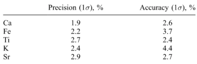
[18] Due to the (necessarily) low sample amount used in this study (50 mg), the digesting performance was tested by duplicate and triplicate sample digests of geostandards and sediment samples covering the entire concentration range where applicable. When there was enough sample powder, ten sediment samples covering the whole concentration range were additionally fused to glass beads and analyzed using conventional XRF spectrometry (Philips PW 2400) according to the routine method described by Schnetger et al. [2000]. Overall analytical precision and accuracy (see Table 1) were tested by (1) replicate digestion and analysis of geostandards GSD-12, PACS-1, GSR-6, several in-house standards and
sediment samples and (2) comparison of ICP-OES and conventional XRF spectrometry data.
2.5. Potential Limitations Using XRF Techniques
[19] The potential limitations of both Micro-XRF and XRF-S are linked to small-scale heterogeneities due to variable porosity, water content, grain-size differences as well as matrix effects (absorption/enhancement) [e.g., Tertian and Claisse, 1982]. These latter effects may occur when part of the emitted fluorescence of Fe and Ti is absorbed or scattered by increasing Ca contents, whereas part of the fluorescence emitted by Ca may additionally excite K.
Table 1. Overall Precision and Accuracy for Analyzed Elements
[20] However, the larger scatter observed for Ti Micro-XRF data (section 2.3) is linked rather to the extremely heterogeneous distribution of minute separate Ti phases as can be seen on the distribution maps (for example, see Figure 8). The larger scatter for K data can be
explained by the fact that the detection of K (the lightest element analyzed) could be influenced by a variety of absorption effects (see the recent work by Kido et al. [2006]). Alternatively, it could be affected by the quality of the film covering the sediment surface: preliminary results based on the element maps showed that total XRF transmission of K was reduced by about 20% when using the PVC thin film compared with Mylar X-ray transmission film. In other words, the element map of K was about 20% darker when using PVC thin film. However, no differences were found for Ca. By contrast, for Ti, Fe and Sr, the Mylar film even reduced the total transmission by 20–25% compared with the PVC film. These findings are rather surprising since Mylar film normally does not affect the transmission of elements with an X-ray energy yield > 4 keV. Since the total attenuation of the Ti signal would have been too high with Mylar film, combined with the other limitations cited above, we hence decided to use the PVC film for our analyses.
[21] Quantitative analyses are typically made more difficult by matrix effects, the interstitial water content and the thin water film formed between the sediment surface and the thin film, especially for light elements such as Al, Si (and K). Kido et al. [2006] recently proposed a correction of these effects by a variety of experiments and calculations. These authors
present a quantification of Al, Si, K, Ca, Ti and Fe by analyzing the cumulative XRF spectra of these elements [Koshikawa et al., 2003] using a similar Micro-XRF (XGT 2700) over intervaled areas of 2.5 cm diameter and comparing their results with those obtained from conventional XRF spectrometry. The samples were selected from two different fine-grained wet marine sediments with a slightly higher range of element concentrations and higher water contents (the latter ranging from 36 to 65%) compared to our study. They estimated the absorption effects caused by the thin film and the thin water film (significant only for Al and Si), as well as the interstitial water and the matrix (effect of Ca on Fe, K and Ti), by analyzing the selected samples in their original wet state and after drying. A principal finding (and important for our study) is that the detection of K with the Micro-XRF is greatly hampered when water contents increase. Even if the water content
of the sediments in our study is 35%, we should still expect a certain effect of the interstitial water on the detection of K. Otherwise, it should be noted that our study is based on the use of XRF element maps (and not the incrementally stepped XRF scans), since it is important to maintain a 100-mm resolution for the structural and mineralogical information contained in the element maps.
3. Results and Discussion
[22] All data discussed here are presented in Tables 2 and 3. It is important to note that we compare data from two different techniques: (1) chemical data (Micro-XRF and XRF-S) obtained from a wet, microscopically uneven and physically/chemically heterogeneous upper layer of sediment of the order of tens to hundreds of microns thick, scanned by the X-ray beam, and (2) chemical data (ICP-OES) obtained from dried and homogenized sediment samples that were then completely dissolved. Therefore the absolute size of the volume scanned by XRF is associated with a certain error due to typical heterogeneity effects. Hence it is quite natural to expect a certain degree of data scatter rather than a perfect correlation between XRF and ICP-OES data.
3.1. Micro-XRF
[23] As mentioned above (section 2.3) and shown in Figures 2 and 3, we adjusted single measurements (element maps and profiles) to the reference overlap map and profile in order to obtain consistent and accurate element profiles for the two sections. To facilitate the comparison between Micro-XRF and ICP-OES data, it was necessary to average the signal over the Micro-XRF map corresponding to the area subsampled for the chemical analysis (see Figure 4). This MicroXRF average value was then plotted against its corresponding ICP-OES data point (Figure 5).
[24] For all elements, we observe an excellent correlation between the Micro-XRF and ICP-OES data (r 2 ! 0.97), except for K (r 2 = 0.89). The value of the intercept is also relatively high for K and Sr. In general, the element concentration range is larger for Section 1 than for Section 2. As shown in Figures 5a and 5e, Sr exhibits the largest concentration range (with no concentration overlap between the two sections), while K exhibits the smallest range. Except for Sr, we obtain higher correlation coefficients for the elements from Section 1 than for those from Section 2 due to their wider concentration ranges. Except for Ca (Figure 5d),
which exhibits a negligible y axis intercept, we observe slightly positive intercepts for Sr and K as well as slightly negative intercepts for Ti and Fe. There is an absence of very low values for Ti, K and Fe (Figures 5b, 5c, and 5e), so the relationship between Micro-XRF and ICP-OES data is not well defined at very low contents, which may also influence the intercept for these three elements. Furthermore, it is clear that the lowest values of K and Ti show the strongest scatter (Figures 5b and 5e), which could also influence the gradient and intercept of the regression line. (Note that very low contents of Fe, Ti and K are not likely to occur in the remainder of the sediment core since the concentration range for these elements is fully covered by the two sections presented here). A further reason for the non-zero intercepts might be related to the matrix effects of Ca on Fe, Ti and K [Tertian and Claisse, 1982]: part of the emitted fluorescence of Fe and Ti may be absorbed or scattered by increasing Ca contents, resulting in a negative intercept for Fe and Ti. By contrast, part of the emitted fluorescence of Ca may additionally excite K resulting in a positive intercept for K. Given all these influencing factors, it is difficult to account for the non-zero values of the intercepts, at least for K and Ti. By contrast, the positive intercept for Sr seems to be well defined, as indicated by the very good correlation coefficient for the very-low-content samples of
Section 2 and the small error on the intercept (Figure 5a). These features might be caused by the generally higher XRF background when using high voltage (50 kV). Nevertheless, the Micro-XRF is hence capable of detecting a quantifiable content of at least 130 ppm Sr (0.013 wt%).
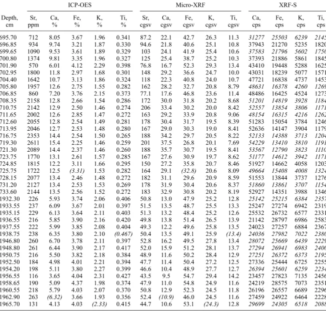
Table 2. Data for Sr, Ca, Fe, K, and Ti Measured With ICP-OES, Micro-XRF, and XRF-S for the Two Sections of Core MD042876 a
A Micro-XRF is the average from 20 data points, given in corrected grayscale values (cgsv). XRF-S is in counts per second (cps). Note that some of the values of the XRF-S (given in italics) are interpolated to fit the depth of ICP-OES and Micro-XRF samples. Four data couples in parentheses/ italics were excluded from the correlation (Figure 3) according to the following reasons: In the case of Fe (Ca), sediment became distinctly darker (lighter) with increasing sampling depth adding a portion of pyrite (carbonate) to the subsample, which was formerly not detected by the XRF beam (which as aforementioned only penetrates the upper 1 mm). In the case of Ti and K we assume a similar sample heterogeneity effect explaining the data inconsistency; however, since Ti and K do not contribute to the sediment color so visibly like Fe and Ca do, this remains unclear. Nevertheless, if these four individual fliers were included in the correlation, the effect on the correlation equation would be completely negligible.
[25] Absorption effects due to water content as well as matrix effects cannot be corrected since they are inherent to the map. As such, they must be put into relation to the averaging of highly heterogeneous areas for profile calculation.
[26] In any case, the very significant correlations observed between the Micro-XRF and ICP-OES data clearly show that all relationships are linear for the concentration range presented here. This is true not only for Ca, Fe and Sr, but also for Ti and K, even if matching between individual Micro-XRF maps is more difficult for the two latter elements (see section 2.3).
3.2. XRF-S
[27] For the quantification of the XRF-S data, we used two different data sets (Tables 2 and 3): the first consists of the data points distributed over the entire core and the second is obtained from both sections (ICP-OES subsamples taken originally for the Micro-XRF data acquisition, see 3.1). The depths (y axis) for the second data set do not always exactly match the depths of the XRF-S data points. Therefore the values for the XRF-S were partly
interpolated (by 2.5 mm) to fit the exact depth of ICP-OES and Micro-XRF samples.
[28] From Figure 6, very good correlations (r 2 ! 0.87) become apparent between chemical data and their correspondent scanner data. The two data sets show very little deviation from each other since they plot in the same area. For all elements, the total concentration range is slightly increased, further supporting the quality of the linear regressions. The second data set exhibits a rather low scatter, even if some data points are interpolated for depth and despite the fact that subsamples are only 2 mm thick, i.e., smaller than the 4 mm XRF-S beam (Figure 4).
[29] Similarly to the Micro-XRF data discussed above, we observe slightly negative intercepts for Fe, Ti and K (Figures 6a, 6c, and 6d), but a slightly positive intercept for Ca (Figure 6b). In the case of Fe, Ti and K, the lowest XRF-S values correspond to the highest Ca values and plot slightly below the respective regression lines. As already mentioned in section 3.1, it is possible that increasing Ca intensities lead to absorption effects that influence the detection of Fe and Ti. The slightly positive intercept for Ca is solely due to the stronger data scatter seen in the second Micro-XRF data set. Indeed, the intercept value calculated with the first data set over the whole core (crossed squares in
Micro-XRF data set. The intercept value calculated with the first data set is À304 ± 732, i.e., also not significantly different Figure 6b) is 1046 ± 1268, i.e., not significantly different from zero. The slightly negative intercept for K (Figure 6c) is also only caused by a stronger data scatter seen in the second Micro-XRF data set. The intercept value calculated with the first
data set is À304 ± 732, i.e., also not significantly different from zero. For Ti and Fe, the negative intercepts of both data sets show no significant difference
Figure 5. Scatterplots for (a) Sr, (b) Ti, (c) Fe, (d) Ca, and (e) K obtained from Micro-XRF (in corrected grayscale values, cgsv) and ICP-OES (in % or ppm). In each legend the correlation coefficient is given for the individual sections. Dashed lines indicate the 95% confidence interval; dotted lines indicate the zero on the y axis. The regression equations are given in
each graph, with corresponding deviations for the gradient and intercept. See also Table 2 and text for further details.
Figure 6. Scatterplots for (a) Fe, (b) Ca, (c) K, and (d) Ti obtained from XRF-S (in kilo counts per second, kcps) and ICP-OES (in %). Windows show samples taken for ICP-OES distributed over the entire core, while black diamonds indicate samples originally taken for the
calibration of Micro-XRF data. Dashed lines indicate the 95% confidence interval; dotted lines indicate the zero on the y axis. The regression equations are given in each graph, with corresponding deviations for the gradient and intercept. See also Tables 2 and 3 and text for further details.
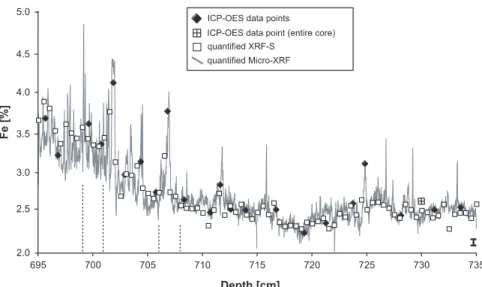
Figure 7. Fe (in %) versus depth for Section 1 as a representative example for the comparison of Micro-XRF, XRF-S, and ICP-OES. The deviation of Micro-XRF and XRF-S data (average 3%, 1s) data is indicated by the error bar (lower right). Dashed lines indicate the segments shown in Figure 8.
3.3. Chemical and Structural Details of Micro-XRF and XRF-S
[30] After calibrating the two XRF-S and MicroXRF data sets, we were able to study in detail the geochemical structure of the sediment core. To see whether the two XRF-S and Micro-XRF data sets match each other as well as the ICP-OES data, we present in Figure 7 a representative example of Fe data plotted versus depth for Section 1. We can see that the profiles obtained by Micro-XRF, XRF-S and ICP-OES plot very close to each other. Even for fine details, the individual XRF-S data points match the Micro-XRF data line very precisely. The discrepancy between Micro-XRF and XRF-S data is generally low ( 3% relative, 1s), demonstrating (1) the overall high technical accuracy and (2) that both non-zero y axis intercepts for the correlation of Micro-XRF and XRF-S Fe (Figures 5c and 6a) have no significant influence on the data quantification.
[31] As mentioned above, one of the major advantages of Micro-XRF is the production of highly detailed element maps. In Figures 8a and 8b, we present two examples (of segments) taken from Section 1 showing all element maps as well as a preliminary element map for sulfur (for which measurement parameters still need calibration). Figure 8a depicts finely laminated sediments, while Figure 8b shows a thick irregularly shaped lamina within a rather homogenous sequence. Light colors correspond to high element contents and dark colors correspond to low element contents. To a first approximation, the contents of Fe, Ti and K decrease while the contents of Ca and Sr increase with depth. Lamination in Figure 8a, for example, is clearly picked out by Fe, Ca and Sr, and, to a somewhat lesser extent, by Ti and K. The thick lamina is rich in Fe, Ti and K but low in Ca and Sr. The very light structures in the sulfur and iron maps indicate the presence of sulfides (usually pyrite). Individual foraminifera tests can be traced by sharp round structures that yield, for example, high Ca, low Sr and approximately zero Fe contents. Distinctly visible minute spots rich in Ti are most likely due to the presence of heavy minerals (e.g., rutile or ilmenite).
[32] Besides sediment input changes, an element profile can also be shaped by dilution by CaCO 3 . A usual way to circumvent the problem is to calculate element profiles on a carbonate free basis. The Ca profile can be used to generate a CaCO 3 profile after
crosschecking with other techniques based on measuring CO 3 . Alternatively, it is possible to consider element ratios. We calculated the Fe/Ti ratio to see whether CaCO 3 dilution is a significant problem in the described section. As seen in Figure 8 the variations in Fe are mostly supported by the Fe/Ti ratio, which indicates that CaCO 3 dilution is not a major effect. In addition, peaks in the Fe/Ti ratio could be either due to changes in background material (i.e., provenance) or due to diagenetically (in situ) formed phases
Figure 8. (a and b) Two segments from Section 1 showing element maps and their corresponding profiles as well as a preliminary map for sulfur contents versus sediment depth. White arrows indicate an individual foraminiferal test (high in Ca, low in Sr). The
presence of diagenetical Fe-sulfides (most likely pyrite) causing peaks in Fe and Fe/Ti is shown by the yellow arrows. The green arrows indicate peaks in Fe and Fe/Ti, which are most likely due to provenance changes. Note also the dispersal of minute Ti-rich phases as indicated in Figure 8b.
such as pyrite. By means of the sulfur maps one can distinguish whether the Fe/Ti signal is related to provenance or diagenetical changes. For example, the highest Fe/Ti peak in Figure 8a is caused by provenance changes, whereas the highest Fe/Ti peak in Figure 8b is due to diagenetical pyrite. This is a clear illustration of the usefulness of both element maps and profiles, leading to unambiguous interpretations.
4. Conclusions and Outlook
[33] With this study, we illustrate the accuracy and usefulness of a recently developed Micro-XRF technique applied to paleo-geochemical research. We present data for Ca, Fe, K, Sr, Ti and S, which were obtained by a Micro-XRF analyzer (MicroXRF) with 100-mm
resolution and by an XRF whole-core scanner (XRF-S) with 5-mm resolution for selected wet sediment sections from a continental margin sediment core. The Micro-XRF technique produces highly resolved two-dimensional element maps. On the basis of overlap
measurements of successive maps, we were able to calculate individual element profiles. We successfully quantified the two XRF data sets using discrete subsamples analyzed by ICP-OES. In this context, we discuss the advantages and limitations of both XRF techniques. A comparison of the two XRF data sets (e.g., using Fe) on a 5-mm resolution demonstrates the overall high consistency and accuracy of all the techniques used. Nevertheless, making use of XRF maps for K and Ti may be difficult for some sediments with high carbonate content, which leads to low K and Ti concentrations and thus reduced precision. Apart from these reservations, the capability to measure elements with a highly focused 100 to 10-mm X-ray beam allows the elemental analysis of single spots, grains or very small areas (such as pyrite, foraminifera tests, Ti-minerals etc.). Overall, element profiles and detailed element maps clearly show that Micro-XRF is a powerful tool for tracing the extent and timing of chemical, mineralogical and sedimentological transitions. Combining Fe/Ti profile and sulfur maps allows discriminating between provenance and diagenetical effects on the Fe profile, which is often a crucial issue in geochemical studies. This example highlights the usefulness of the XRF maps and clearly distinguishes the Micro-XRF from other technical devices producing elemental profiles only. Since Fe (and other redox-sensitive metals) are typically enriched close to diagenetical fronts, as best seen in turbidites and sapropels, the Micro-XRF is thus a very promising tool for analyzing metal contents in such sediments.
Acknowledgments
[34] We thank Ursula Ro¨hl (University of Bremen) for giving access to the XRF core scanner and Heike Pfletschinger, who kindly provided technical assistance. Hans-Ju¨rgen Brumsack and Bernhard Schnetger are thanked for giving access to the chemical facilities and the ICP-OES at the ICBM (University of Oldenburg). We are also grateful to Perrine Chaurand (CEREGE, University Paul Ce´zanne) for technical suggestions concerning the Micro-XRF. Helpful comments by the reviewers Hans-Ju¨rgen Brumsack and Martin Ko¨lling are
the ANR, the Gary Comer Science and Education Foundation, and the European Community (project STOPFEN, HPRN-CT-2002-0221).
References
Haug, G. H., D. Gu¨nther, L. C. Peterson, D. M. Sigman, K. A. Hughen, and B. Aeschlimann (2003), Climate and the collapse of Maya civilization, Science, 299(5613), 1731–1735.
Heinrichs, H., and A. G. Herrmann (1990), Praktikum der Analytischen Geochemie, Springer, New York.
Hosokawa, Y., S. Ozawa, H. Nakasawa, and T. Nakayama (1997), An X-ray guide tube and a desk-top scanning X-ray analytical microscope, X-Ray Spectrom., 26, 380–387.
Jansen, J. H. F., S. J. Van der Gaast, B. Koster, and A. J. Vaars (1998), CORTEX, a shipboard XRF-scanner for element analyses in split sediment cores, Mar. Geol., 151(1–4), 143–153.
Kido, Y., T. Koshikawa, and R. Tada (2006), Rapid and quantitative major element analysis method for wet fine-grained sediments using an XRF microscanner, Mar. Geol., 229(3–4), 209–225, doi:10.1016/j.margeo.2006.03.002.
Koshikawa, T., Y. Kido, and R. Tada (2003), High-resolution rapid elemental analysis using an XRF microscanner, J. Sediment. Res., 73(5), 824–829.
Peterson, L. C., G. H. Haug, K. A. Hughen, and U. Ro¨hl (2000), Rapid changes in the
hydrologic cycle of the tropical Atlantic during the last glacial, Science, 290(5498), 19471951.
Ro¨hl, U., and L. J. Abrams (2000), High resolution, downhole, and non-destructive core measurements from sites 999 and 1001 in the Caribbean Sea: application to the Late Paleocene Thermal Maximum, Proc. Ocean Drill. Program Sci. Results, 165, 191–204.
Rose, J., et al. (2006), Applications of a 10 mm spot size laboratory Micro-XRF to environmental sciences, paper presented at EXRS European Conference on X-Ray Spectrometry, CEA-LIST-LNHB, Paris, 19 –23 June .
Schnetger, B., H. J. Brumsack, H. Schale, J. Hinrichs, andL. Dittert (2000), Geochemical characteristics of deep-sea sediments from the Arabian Sea: A high-resolution study, Deep Sea Res., Part II, 47, 2735–2768.
Tertian, R., and F. Claisse (1982), Principles of Quantitative X-Ray Fluorescence Analysis, 319 pp., Heyden, London. von Rad, U., A. Khan, W. H. Berger, D. Rammlmaier, and
U. Treppke (2002), Varves, turbidites and cycles in upper Holocene sediments (Makran slope, northern Arabian Sea), in The Tectonic and Climatic Evolution of the Arabian Sea Region, edited by P. D. Clift et al., Geol. Soc. Spec. Publ., 195, 387–406.