HAL Id: hal-02879626
https://hal.archives-ouvertes.fr/hal-02879626
Submitted on 24 Jun 2020
HAL is a multi-disciplinary open access
archive for the deposit and dissemination of sci-entific research documents, whether they are pub-lished or not. The documents may come from teaching and research institutions in France or abroad, or from public or private research centers.
L’archive ouverte pluridisciplinaire HAL, est destinée au dépôt et à la diffusion de documents scientifiques de niveau recherche, publiés ou non, émanant des établissements d’enseignement et de recherche français ou étrangers, des laboratoires publics ou privés.
SOLUTION OF LINEAR FRACTIONAL PARTIAL
DIFFERENTIAL EQUATIONS BASED ON THE
OPERATOR MATRIX OF FRACTIONAL
BERNSTEIN POLYNOMIALS AND ERROR
CORRECTION
Wenhui Li, Ling Bai, Yiming Chen, Serge Santos, Baofeng Li
To cite this version:
Wenhui Li, Ling Bai, Yiming Chen, Serge Santos, Baofeng Li. SOLUTION OF LINEAR FRAC-TIONAL PARTIAL DIFFERENTIAL EQUATIONS BASED ON THE OPERATOR MATRIX OF FRACTIONAL BERNSTEIN POLYNOMIALS AND ERROR CORRECTION. International Jour-nal of Innovative Computing and Applications, Inderscience Publishers, 2018, 14, pp.211 - 226. �hal-02879626�
Computing, Information and Control ICIC International c⃝2018 ISSN 1349-4198
Volume 14, Number 1, February 2018 pp. 211–226
SOLUTION OF LINEAR FRACTIONAL PARTIAL DIFFERENTIAL EQUATIONS BASED ON THE OPERATOR MATRIX
OF FRACTIONAL BERNSTEIN POLYNOMIALS AND ERROR CORRECTION
Wenhui Li1,2, Ling Bai3, Yiming Chen3,4,5, Serge Dos Santos6 and Baofeng Li7
1School of Information Science and Engineering
2The Key Laboratory for Special Fiber and Fiber Sensor of Hebei Province 3College of Science
Yanshan University
No. 438, Hebei Avenue, Qinhuangdao 066004, P. R. China 799432279@qq.com
4Le Studium
Loire Valley Institute for Advanced Studies 1 rue Dupanloup, Orl´eans 45000, France
5Laboratoire PRISME
INSA – Institut National des Sciences Appliqu´ees University of Orleans
Boulvevard Lahitolle, Bourges 18000, France
6INSA Centre Val de Loire
University of Orleans
PRISME EA 4229, Bourges Cedex 18022, France
7College of Sciences
Tangshan Normal University
No. 156, Jianshe North Road, Tangshan 063000, P. R. China Received April 2017; revised August 2017
Abstract. In this paper, firstly, a new method which makes a modification of the Bern-stein polynomials is introduced to solve the linear fractional partial differential equations (FPDEs). The biggest advantage of the fractional Bernstein polynomials is that the order can be changed with the order of the fractional partial differential equations. For the first time, we try to use this method to solve the linear fractional partial differential equations. Secondly, convergence analysis and error correction are also given to make the calcula-tion results more accurate. The concrete content of this method and error correccalcula-tion are explained briefly and numerical examples are given to demonstrate the validity and accuracy of the method.
Keywords: Fractional Bernstein polynomials, Linear fractional partial differential
equa-tion, Operator matrix, Convergence analysis, Error correction
1. Introduction. Since 1974, Oldam and Spanier published the first book on the the-ory of fractional order calculus book [1], and the fractional order calculus is developed quickly. At present, the main definitions of fractional operator include Riemann-Liouvile, Caputo, Grunwald-Letnikov, Weyl, Erdelyi-Kober, Riesz and Marchaud-Hadamard [2, 3]. With the efforts of many scholars, fractional order calculus theory to a certain extent was established. Modeling problem in the field of engineering as well as the complex mechanics, physics problems promoted fractional order calculus theory and application
research, and in these problems, fractional calculus had certain practical significance and geometric interpretation. In soft matter physics, environmental mechanics, non-Newton fluid mechanics, viscous elastic mechanics, porous media dynamics and anomalous diffu-sion, fractional order differential research has caused a high degree of attention, and at the same time, it has been widely used. For fractional calculus, an important part is the study of fractional differential equation. When talking about the equation, solution is an inevitable problem. Due to the fact that overwhelming majority of the accurate solution of fractional differential equations is not easy to get, more and more scholars dedicated to studying its numerical solution. The most commonly used methods are like variational it-eration method [4], finite difference method [5], generalized differential transform method [6, 7], Adomian decomposition method [8, 9], wavelet method [10] and operational matrix method [11, 12], for example, Adomian decomposition method, the homotopy perturba-tion method, the homotopy analysis method, the variaperturba-tional iteraperturba-tion method, the wavelet operator matrix analysis method, and block pulse function method. In [13], Wang et al. solved the fractional differential equation based on the Bernstein polynomials, proving the feasibility of the Bernstein polynomial for fractional differential equation. In [14], Chen et al. solved the FPDEs based on the fractional Legendre polynomial, introducing some theories to the fractional partial differential equations. Based on these, first, we will construct a class of fractional orthogonal polynomial (namely fractional Bernstein polyno-mial) with the help of Bernstein polynomial. Then, by using the properties of fractional calculus, we deduce the fractional differential operator matrix. At last, we combine the operator matrix and collocation method [15] to solve the FPDEs. Compared with [13], the maximum advantage of this method is that the order of polynomials used to approximate functions has variability with the order of the equation, which makes this method more flexible. Compared with [14], in this paper, the Bernstein polynomial is more conciseness than Legendre polynomial, which increases the calculation speed and accuracy. In this chapter, we consider the FPDEs on Ω = [0, 1]× [0, 1]
∂υu(x, t)
∂xυ +
∂γu(x, t)
∂tγ = g(x, t) (1)
u(0, t) = u(x, 0) = 0 (2)
where u(x, t) is unknown function and g(x, t) is known function, and υ and γ are the order. This paper is organized as follows. In Section 2, some definitions of fractional calculus are presented. In Section 3, we give the definition and matrix form of fractional Bernstein polynomial. And we introduce the theory of two-dimensional function approximation. In Section 4, we present the error analysis and error correction. In Section 5, we use the method to deduce the fractional differential operator matrix and find the fundamental matrix equation, and use collocation points to obtain a linear system. Next, correction solution is obtained through the error correction. In Section 6, two numerical examples are presented in order to support our work. The paper is concluded in Section 7 by a brief conclusion.
2. Preliminaries and Notations. In this section, we give some definitions of the frac-tional calculus.
Definition 2.1. [16] A real α, [α] is the biggest integer which [α] ≤ α, if f(t) is defined
[a, t] has m + 1 order continuous derivative, when α>0, m is α at least, and the α order
derivative of f (t) is defined as follows: G aDαtf (t) = lim h→0, mh=t−ah −α∑m k=0 gkf (t− kh) (3)
where G
aDαt is the derivative operator, G represents Grunwald-Letnikov (G-L), α is the
order, a and t are integral lower bound and higher bound respectively, and α is initial value of t, constant gk = (−α)(−α+1)(−α+2)···(−α+k−1)k! .
Because α>0, (3) is given as: G aD α tf (t) = m ∑ k=0 fk(a)(t− a)−α+k Γ(−α + k + 1) + 1 Γ(−α + k + 1) ∫ t a (t− τ)m−αfm+1(τ ) dτ (4)
where Γ(α) =∫0∞e−xxα−1dx = (α− 1)! is gamma function.
In order to simplify the calculation in the practical application, under the premise that satisfies the conditions and properties of fractional calculus, on the basis of G-L definition, we can find the improved Riemann-Liouville (R-L) calculus.
Definition 2.2. [17] If f (t) is a continuous function on the interval [0, +∞), namely
f (t) ∈ C[0, +∞), and is integrable on any finite subinterval of [0, +∞), so R-L integral
is defined as R aD−βt f (t) = f (t) β = 0 1 Γ(β) ∫ t a f (τ ) (t− τ)1−β dτ β > 0, τ > 0 (5)
in order to distinguish, the R
aD−βt becomes I β t, so (5) can be written as Iβtf (t) := 1 Γ(β) ∫ t a τβ−1f (t− τ) dt β > 0 (6)
α order R-L differential definition as
R aD α tf (t) = dnf (t) dtn α = n∈ N dn dtn 1 Γ (n− α) ∫ t a f (τ ) (t− τ)α−n+1dτ 0≤ n − 1 < α < n (7)
Definition 2.3. [18] If f (t)∈ Cn(0, +∞), the Caputo fractional derivative is
C aD α tf (t) = dnf (t) dtn α = n∈ N + 1 Γ(n− α) ∫ t a f(n)(τ ) (t− τ)α−n+1dτ 0≤ n − 1 < α < n (8)
where CaDαt is Caputo fractional differential operator. In this paper, we use the Caputo
definition. In order to be convenient, we use Dα to represent it.
Particularly, when f (t) = tm, Dαxm = 0 α∈ N and m < ⌈α⌉ Γ (m + 1) Γ (m + 1− α)x x−α m∈ N 0 and m≥ ⌈α⌉ or m /∈ N and m > ⌊α⌋ (9) where N0 ={0, 1, 2, . . .}, N = {1, 2, . . .}. Upper limit function ⌈α⌉ is the smallest positive
integral where ⌈α⌉ > α; lower limit function ⌊α⌋ is the biggest positive integral where
3. Fractional Bernstein Polynomial and Function Approximate.
3.1. Fractional Bernstein polynomial. We can find the definitions of Bernstein poly-nomial in [9, 10, 11, 12, 13] as follows.
Definition 3.1. [18, 19] n order Bernstein polynomial in [0, 1] is
Bi,n(x) = ( n i ) xi(1− x)n−i (10)
Using binomial theorem in (10), we can obtain Bi,n(x) = n−i ∑ k=0 (−1)k ( n i )( n− i k ) xi+k (11)
Definition 3.2. [19, 20] n order Bernstein polynomial in [0, R] is
Bi,n(x) = ( n i ) xi(R− x)n−i Rn = n−i ∑ k=0 (−1)k ( n i )( n− i k ) xi+k Ri+k (12)
Definition 3.3. [21, 22] n order Bernstein polynomial in [a, b] is
Bi,n(x) = ( n i ) (x− 1)i(b− x)n−i (b− a)n (13)
Substituting x→ xα in (10), we can obtain fractional Bernstein polynomial is [0, 1] as
follows: Bi,nα (x) = ( n i ) xiα(1− xα)n−i = n−i ∑ k=0 (−1)k ( n i )( n− i k ) x(i+k)α (14)
Then, we deduce the matrix form of fractional Bernstein polynomial:
Φ(x) =[B0,nα (x), Bα1,n(x), . . . , Bn,nα (x)]T = AX (15) where A = (−1)0(n0)(n0) (−1)1(n0)(n1) · · · (−1)n−0(n0)(nn−0−0) 0 (−1)0(n1)(n−10 ) · · · (−1)n−1(n1)(nn−1−1) .. . ... . .. ... 0 0 · · · (−1)0(nn) (16) X = [1, xα, . . . , xnα] (17)
3.2. Two-dimensional function approximation theory. We can find one-dimensio-nal function approximation based on fractioone-dimensio-nal Bernstein polynomial in [15].
Square-integrable function u(x) ∈ [0, xu] can be approximated, and we consider the n + 1 terms. u(x)≈ n ∑ i=0 ciBi,nα (x) = CTΦ(x) (18) where C = [c0, c1, . . . , cn] T
is coefficient matrix which needs to obtain. C also can be obtained by C = Q−1⟨u, Φ(x)⟩, and ⟨∗⟩ is defined ⟨u, Φ(x)⟩ =∫0xuu(x)Φ(x)dx where
Q = ∫ xu 0 Φ (x) ΦT(x) dx = ∫ xu 0 (AX) (AX)T dx = A (∫ xu 0 XXTdx ) AT = AHAT
Two-dimensional function approximation based on Bernstein polynomial exists in [23, 24]. Now, we give the two-dimensional function approximation based on fractional Bern-stein polynomial as follows.
If u(x, t)∈ L2([0, 1)× [0, 1)) considers n + 1 terms,
u(x, t)≈ n ∑ i=0 n ∑ j=0 ui,jBi,nα (x)B β j,n(t) = Φ T(x)U Φ(t) (19)
where ui,j (i = 0, 1, . . . , n; j = 0, 1, . . . , n) is undetermined coefficient
U = u00 u01 · · · u0n u10 u11 · · · u1n .. . ... . .. ... un0 un1 · · · unn (20)
The U can be obtained by the equation of U = Q−1⟨Φ(x), ⟨Φ(t), u(x, t)⟩⟩ Q−1. 4. Convergence Analysis and Error Correction.
4.1. Convergence analysis. We can find the error analysis about approximation based on Bernstein polynomial in [21, 25, 26]. Now, we deduce the error analysis about approx-imation based on fractional Bernstein polynomial.
Theorem 4.1. [21, 25, 26] If H is Hilbert space, Y is random subspace, and dim Y <∞.
If {y1, y2, . . . , yn} ∈ Y is a set of orthogonal basis, x ∈ H, y0 is the best approximation of
x∈ Y , ∥x − y0∥22 = G (x, y1, y2, . . . , yn) G (y1, y2, . . . , yn) (21) where G (x, y1, y2, . . . , yn) = ⟨x, x⟩ ⟨x, y1⟩ · · · ⟨x, yn⟩ ⟨y1, x⟩ ⟨y1, y1⟩ · · · ⟨y1, yn⟩
..
. ... . .. ...
⟨yn, x⟩ ⟨yn, y2⟩ · · · ⟨yn, yn⟩
(22)
Corollary 4.1. [21, 25, 26] If Y = Span{B0,nα , B1,nα , . . . , Bn,nα }, the absolute error in Theorem 4.1 can be written as
∥x − y0∥ = det[∫xxu 0 Ψ(x)Ψ T(x) dx] det[∫xxu 0 Φ(x)Φ T(x) dx ] (23) where ΨT =[x, B0,nα , B1,nα , . . . , Bn,nα ] and ΦT =[B0,nα , B1,nα , . . . , Bn,nα ] (24) Theorem 4.2. If g ∈ Cn+1[x 0, xu] and Y = Span { Bα 0,n, B1,nα , . . . , Bn,nα } , CTΦ(x) is the best approximation of g in Y , so the biggest error is
g− CTΦ (x) 2 ≤ M (xu− x0)
2n+3 2
(n + 1)√2n + 3 (25)
where M = maxx∈[x0,xu] g
Proof: The Taylor expansion of g(x) is g1(x) = g(x0) + g′(x0) (x− x0) + g′′(x0) (x− x0)2 2 +· · · + g (n) (x0) (x− x0)n n! (26)
Using Lagrange mean value theorem, we can obtain
|g(x) − g1(x)| = g(n+1)(x) (x − x 0)n+1
(n + 1)! ∃ϵ ∈ (x0, xu) (27)
CTΦ(x) is the best approximation of g in Y , so
g− CTΦ(x) 2 2 ≤ ∥g − y1∥ 2 2 = ∫ xu x0 |g − y1(x)|2 dx ≤ ∫ xu x0 [ g(n+1)(ϵ) (x − x0) n+1 (n + 1)! ]2 dx ≤ M2 (n + 1)!2 ∫ xu x0 (x− x0)2n+2dx = M 2(x u− x0) 2n+3 (n + 1)!2(2n + 3) (28)
After square, we can obtain the biggest error, end.
Definition 4.1. f ∈ [a, b], the convergence coefficient form is
ω(f, δ) = sup
x,y∈[a,b],|x−y|≤δ
|f(x) − f(y)| (29)
Theorem 4.3. [21, 25, 26] f ∈ [a, b] is uniform convergence if and only if
lim
δ→0ω(f, δ) = 0 (30)
Theorem 4.4. [21, 25, 26] f ∈ [0, 1] and bound, so ∥f − p(f, n)∥∞ ≤ 3 2ω ( f,√1 n ) where p(f, n) =∑nk=0f(kn)Bα k,n and ∥f∥∞= sup|f(x)|.
Theorem 4.5. [21, 25, 26] If f ∈ [0, 1] satisfies α order Lipschitz condition,
∥f − p(f, n)∥∞≤ 3
2km
−α
2 (31)
where k is Lipschitz constant.
Theorem 4.6. If f ∈ [0, 1] and bound, Y = Span{Bα
0,n, B1,nα , . . . , Bn,nα
}
, if CTΦ(x) is the best approximation of f in Y ,
f− CTΦ ∞ ≤ 3 2ω ( f,√1 n ) (32)
Proof: Because CTΦ(x) is the best approximation of f in Y and p(f, m) ∈ Y ,
combin-ing ∥f∥2 ≤ ∥f∥∞, we can obtain
f− CTΦ 2 ≤ ∥f − p(f, n)∥2 ≤ ∥f − p(f, n)∥∞ ≤ 3 2ω ( f,√1 n ) (33)
4.2. Error correction. First, we assume that u∗(x, t) is the approximate solution of Equation (1) and Equation (2). Thus, u∗(x, t) satisfies the problem ∂υu∂x∗(x,t)υ +
∂γu ∗(x,t)
∂tγ =
g(x, t). And u(x, t) is the exact solution of Equation (1) and Equation (2). So, we define
the error function as
e(x, t) = u(x, t)− u∗(x, t) (34)
Next, we write Equation (1) for L [u(x, t)] = ∂υ∂xu(x,t)υ +
∂γu(x,t)
∂tγ = g(x, t). Thus, we can
define residual items as R∗(x, t) = L [u∗(x, t)]− g(x, t). So, we can obtain
L [u∗(x, t)] = R∗(x, t) + g(x, t) (35) Because u(x, t) is the exact solution, there are no residual items, namely residual item is 0, and we can obtain
L [u(x, t)] = 0 + g(x, t) (36)
Then, through Equation (34), Equation (35) and Equation (36), we can infer error fractional partial differential equations as follows:
L [e∗(x, t)] = L [u(x, t)]− L [u∗(x, t)] = 0 + g(x, t)− R∗(x, t)− g(x, t) =−R∗(x, t) (37) Namely: ∂υe(x, t) ∂xυ + ∂γe(x, t) ∂tγ =−R∗(x, t) (38)
Here, e∗(x, t) is exact solution of Equation (38). We can obtain approximate solution
e∗∗(x, t) of Equation (38) by some methods.
Last, approximate solution u∗(x, t) plus error approximate solution e∗∗(x, t) is defined correction solution u∗∗(x, t), namely:
u∗∗(x, t) = u∗(x, t) + e∗∗(x, t) (39) 5. Numerical Method. First, we deduce the fractional differential operator matrix of fractional Bernstein polynomial. Combining Equation (9) and Equation (15), we can obtain DαΦ (x) = DαAX = ADαX = ADα 1 xα .. . xnα = A Dα1 Dαxα .. . Dαxnα = A 0 Γ (α + 1) Γ (2α + 1) Γ (α + 1) x α .. . Γ (nα + 1) Γ ((n− 1) α + 1)x (n−1)α = A 0 0 0 · · · 0 0 Γ (α + 1) 0 · · · 0 0 0 Γ (2α + 1) Γ (α + 1) · · · 0 .. . ... ... . .. ... 0 0 0 · · · Γ (nα + 1) Γ ((n− 1) α + 1) 0 1 xα .. . x(n−1)α
= AP 0 0 · · · 0 0 1 0 · · · 0 0 0 1 · · · 0 0 .. . ... . .. ... ... 0 0 · · · 1 0 1 xα .. . xnα = A∗ P ∗ E1 ∗ X = A ∗ P ∗ E1 ∗ A−1∗ Φ (x) (40) So Dα= A∗ P ∗ E1 ∗ A−1 (41) where P = 0 0 0 · · · 0 0 Γ (α + 1) 0 · · · 0 0 0 Γ (2α + 1) Γ (α + 1) · · · 0 .. . ... ... . .. ... 0 0 0 · · · Γ (nα + 1) Γ ((n− 1) α + 1) (42) E1 = 0 0 · · · 0 0 1 0 · · · 0 0 0 1 · · · 0 0 .. . ... . .. ... ... 0 0 · · · 1 0 (43)
Then, combining Equation (19) and Equation (41), we can obtain
∂υu (x, t) ∂xυ ∼= ∂υ(ΦT (x) U Φ (t)) ∂xυ = ( ∂υΦ (x) ∂xυ )T U Φ (t)≈ ΦT(x) (Dυ)T U Φ (t) (44) ∂γu (x, t) ∂tγ ∼= ∂γ(ΦT (x) U Φ (t)) ∂xγ = Φ T (x) U∂γΦ (t) ∂tγ ≈ Φ T (x) U DγΦ (t) (45) where Dυ = A∗ M ∗ E1 ∗ A−1 (46) M = 0 0 0 · · · 0 0 Γ (υ + 1) 0 · · · 0 0 0 Γ (2υ + 1) Γ (υ + 1) · · · 0 .. . ... ... . .. ... 0 0 0 · · · Γ (nυ + 1) Γ ((n− 1) υ + 1) (47) Dγ = A∗ N ∗ E1 ∗ A−1 (48) N = 0 0 0 · · · 0 0 Γ (γ + 1) 0 · · · 0 0 0 Γ (2γ + 1) Γ (γ + 1) · · · 0 .. . ... ... . .. ... 0 0 0 · · · Γ (nγ + 1) Γ ((n− 1) γ + 1) (49) u (0, t) ∼= ΦT (0) U Φ (t) (50)
u (x, 0) ∼= ΦT (x) U Φ (0) (51) Using Equation (44) to Equation (51) in Equation (1) and Equation (2), we can deduce the initial fractional partial differential equation as follows:
ΦT (x) (Dυ)TU Φ (t) + ΦT (x) U Dγ TΦ (t) = g (x, t) (52)
ΦT(0) U Φ (t) = ΦT (x) U Φ (0) = 0 (53)
Finally, discrete variable (x, t)→ (xi, ti) by collocation method is xi =
2ki− 1
2n and ti =
2ki− 1
2n (i = 1, 2, . . . , n) (54)
so Equation (52) and Equation (53) become system of linear equations. Combining Mat-lab and least square fitting, we can obtain the undetermined coefficient ui,j. Through
Equation (19) we deduce the numerical solution of Equation (1) to Equation (2). 6. Numerical Example.
Example 6.1. Considering the fractional partial differential equation as
∂14u (x, t) ∂x14 +∂ 1 2u (x, t) ∂t12 = g (x, t) (55) u (0, t) = u (x, 0) = 0 (56)
the exact solution is x2t2, where g (x, t) = 8x2t32
3√π +
32t2x74
21Γ(34).
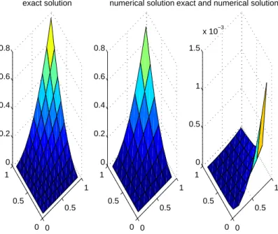
The exact solution, numerical solution, exact and numerical solution error, approximate solution of error, correction solution and exact and correction solution error for different n = 4, ne = 7; n = 5, ne = 8; n = 6, ne = 8 are reported in Figures 1-6. What can be found in these images is that the correction solution by error correction is closer to the exact solution than the previous numerical solution, which shows that the error correction can reduce the error. And with the increase of the number of nodes selected, the accuracy
0 0.5 1 0 0.5 1 0 0.2 0.4 0.6 0.8 exact solution 0 0.5 1 0 0.5 1 −0.2 0 0.2 0.4 0.6 0.8 numerical solution 0 0.5 1 0 0.5 1 0 0.005 0.01 0.015
exact and numerical solution error
Figure 1. Exact solution, numerical solution and exact and numerical solution error to Example 6.1, for n = 4, ne = 7
0 0.5 1 0 0.5 1 −0.2 0 0.2 0.4 0.6 0.8
approximate solution of error
0 0.5 1 0 0.5 1 0 0.2 0.4 0.6 0.8 correction solution 0 0.5 1 0 0.5 1 0 0.5 1 1.5 x 10⁻⁴
exact and correction solution error
Figure 2. Approximate solution of error, correction solution and exact and correction solution error to Example 6.1, for n = 4, ne = 7
0 0.5 1 0 0.5 1 0 0.2 0.4 0.6 0.8 exact solution 0 0.5 1 0 0.5 1 −0.2 0 0.2 0.4 0.6 0.8 numerical solution 0 0.5 1 0 0.5 1 0 1 2 3 4 5 6 x 10⁻³
exact and numerical solution error
Figure 3. Exact solution, numerical solution and exact and numerical solution error to Example 6.1, for n = 5, ne = 8
of the solution has been improved. The results show the validity and applicability of the presented method and error correct, and we can obtain more accurate solution.
Example 6.2. Considering the fractional partial differential equation as
∂54u (x, t) ∂x54 +∂ 5 4u (x, t) ∂t54 = g (x, t) (57) u (0, t) = u (x, 0) = 0 (58)
0 0.5 1 0 0.5 1 −0.2 0 0.2 0.4 0.6 0.8
approximate solution of error
0 0.5 1 0 0.5 1 0 0.2 0.4 0.6 0.8 correction solution 0 0.5 1 0 0.5 1 0 0.5 1 1.5 2 2.5 x 10⁻⁶
exact and correction solution error
Figure 4. Approximate solution of error, correction solution and exact and correction solution error to Example 6.1, for n = 5, ne = 8
0 0.5 1 0 0.5 1 0 0.2 0.4 0.6 0.8 exact solution 0 0.5 1 0 0.5 1 0 0.2 0.4 0.6 0.8 numerical solution 0 0.5 1 0 0.5 1 0 0.5 1 1.5 x 10⁻³
exact and numerical solution error
Figure 5. Exact solution, numerical solution and exact and numerical solution error to Example 6.1, for n = 6, ne = 8
the exact solution is x52t 5 4 + x 5 4t 15 4 , where g (x, t) = 5Γ(14) 16 x 5 2 + 5Γ(14) 16 t 15 4 + 30 √πx5 4t54 16Γ(94) + 2x54t52Γ(15 4) √π .
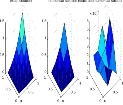
The exact solution, numerical solution, exact and numerical solution error, approximate solution of error, correction solution and exact and correction solution error for different n = 3, ne = 5; n = 5, ne = 7; n = 6; ne = 7 are reported in Figures 7-12. In these
0 0.5 1 0 0.5 1 −0.2 0 0.2 0.4 0.6 0.8
approximate solution of error
0 0.5 1 0 0.5 1 0 0.2 0.4 0.6 0.8 correction solution 0 0.5 1 0 0.5 1 0 0.5 1 1.5 2 x 10⁻⁶
exact and correction solution error
Figure 6. Approximate solution of error, correction solution and exact and correction solution error to Example 6.1, for n = 6, ne = 8
0 0.5 1 0 0.5 1 0 0.5 1 1.5 exact solution 0 0.5 1 0 0.5 1 0 0.5 1 1.5 numerical solution 0 0.5 1 0 0.5 1 0 1 2 3 4 5 6 x 10⁻⁹
exact and numerical solution error
Figure 7. Exact solution, numerical solution and exact and numerical solution error to Example 6.2, for n = 3, ne = 5
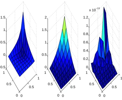
images, we can also find the correction solution by error correction is closer to the exact solution than the previous numerical solution, which shows that the error correction can reduce the error. And we can get very high resolution by picking very few nodes n. The results show the validity and applicability of the presented method and error correct, and we can obtain more accurate solution.
0 0.5 1 0 0.5 1 −0.5 0 0.5 1 1.5
approximate solution of error
0 0.5 1 0 0.5 1 0 0.5 1 1.5 correction solution 0 0.5 1 0 0.5 1 0 0.5 1 1.5 x 10⁻¹⁴
exact and correction solution error
Figure 8. Approximate solution of error, correction solution and exact and correction solution error to Example 6.2, for n = 3, ne = 5
0 0.5 1 0 0.5 1 0 0.5 1 1.5 2 exact solution 0 0.5 1 0 0.5 1 0 0.5 1 1.5 numerical solution 0 0.5 1 0 0.5 1 0 2 4 6 8 x 10⁻⁸
exact and numerical solution error
Figure 9. Exact solution, numerical solution and exact and numerical solution error to Example 6.2, for n = 5, ne = 7
7. Conclusions. In this paper, first according to the theory of function approximation with fractional Bernstein polynomial approximate unknown functions u (x, t); then frac-tional differential operator matrix of fracfrac-tional Bernstein polynomial is derived by using the properties of fractional calculus; next combining the ideas of the operator matrix and collocation method to discrete variable (x, t) become (xi, ti), converting the problem
to solve the algebraic equations and obtaining the numerical u∗(x, t); then by using the residual function, an error fractional partial differential equation is constructed and thus
0 0.5 1 0 0.5 1 −0.5 0 0.5 1 1.5
approximate solution of error
0 0.5 1 0 0.5 1 0 0.5 1 1.5 2 correction solution 0 0.5 1 0 0.5 1 0 0.5 1 1.5 x 10⁻¹²
exact and correction solution error
Figure 10. Approximate solution of error, correction solution and exact and correction solution error to Example 6.2, for n = 5, ne = 7
0 0.5 1 0 0.5 1 0 0.5 1 1.5 2 exact solution 0 0.5 1 0 0.5 1 0 0.5 1 1.5 numerical solution 0 0.5 1 0 0.5 1 0 0.2 0.4 0.6 0.8 1 x 10⁻⁷
exact and numerical solution error
Figure 11. Exact solution, numerical solution and exact and numerical solution error to Example 6.2, for n = 6, ne = 7
the approximate solution of error obtained by fractional Bernstein polynomial is corrected as e∗∗(x, t), and we can obtain the correction solution u∗(x, t) + e∗∗(x, t); at last two nu-merical examples are given to prove the feasibility and effectiveness of the method and we can obtain more accurate solution by error correct, and we can find high accuracy as long as small n and ne. In the future, we can try to apply this method to studying the partial differential equation of variable coefficient, and expand the applicability of this method.
0 0.5 1 0 0.5 1 −0.5 0 0.5 1 1.5
approximate solution of error
0 0.5 1 0 0.5 1 0 0.5 1 1.5 2 correction solution 0 0.5 1 0 0.5 1 0 0.2 0.4 0.6 0.8 1 1.2 x 10⁻¹³
exact and correction solution error
Figure 12. Approximate solution of error, correction solution and exact and correction solution error to Example 6.2, for n = 6, ne = 7
Acknowledgment. This work is supported by the Natural Science Foundation of Hebei
Province (A2017203100) in China and the Le Studium Research Professorship award of Centre-Val de Loire region in France.
REFERENCES
[1] A. B. Malinowska and D. F. M. Torres, Generalized natural boundary conditions for fractional variational problems in terms of the Caputo derivative, Computers & Mathematics with Applications, vol.59, no.9, pp.3110-3116, 2010.
[2] E. Sousa, Finite difference approximations for a fractional advection diffusion problem, Journal of Computational Physics, vol.228, pp.4038-4054, 2009.
[3] A. A. Kilbas, H. M. Srivastava and J. J. Trujillo, Theory and applications of fractional differential equations, Elsevier, vol.51, pp.151-173, 2006.
[4] Z. M. Odibat, A study on the convergence of variational iteration method, Math. Comput. Model, vol.51, pp.1181-1192, 2010.
[5] Y. Zhang, A finite difference method for fractional partial differential equation, Applied Mathematic Letters, vol.215, pp.524-529, 2009.
[6] Z. Odibat and S. Momani, Generalized differential transform method: Application to differential equations of fractional order, Appl. Math. Comput., vol.197, pp.467-477, 2008.
[7] S. Momani and Z. Odibat, Generalized differential transform method for solving a space and time-fractional diffusion-wave equation, Phys. Lett. A, vol.370, pp.379-387, 2007.
[8] I. L. El-Kalla, Convergence of the Adomian method applied to a class of nonlinear integral equations, Appl. Math. Comput., vol.21, pp.372-376, 2008.
[9] M. M. Hosseini, Adomian decomposition method for the solution of nonlinear differential algebraic equations, Appl. Math. Comput., vol.181, pp.1737-1744, 2006.
[10] Y. M. Chen, Y. B. Wu et al., Wavelet method for a class of fractional convection diffusion equation with variable coefficients, Comput. Sci., vol.1, pp.146-149, 2010.
[11] M. Yi, J. Huang and J. Wei, Block pulse operational matrix method for solving fractional partial differential equation, Appl. Math. Comput., vol.221, pp.121-131, 2013.
[12] J. L. Wu, A wavelet operational method for solving fractional partial differential equations numeri-cally, Appl. Math. Comput., vol.214, pp.31-40, 2009.
[13] J. Wang, L. Liu, Y. Chen and X. Ke, Numerical solution for fractional partial differential equation with Bernstein polynomial, Journal of Electronic and Technology, vol.12, pp.331-338, 2014.
[14] Y. Chen, Y. Sun, L. Liu and X. Ke, Numerical solution of the fractional partial differential equations by the fractional-order Legendre funtions, Computer Modeling in Engineering & Science, vol.244, pp.847-858, 2014.
[15] M. H. T. Alshbool and A. S. Bataineh, Solution of fractional-order differential equations based on the operational matrices of new fractional Bernstein functions, Journal of King Saud University-Science, vol.28, no.4, pp.273-400, 2016.
[16] S. G. Samko, A. A. Kilbas and O. A. Marichev, Fractional Integrals and Derivatives: Theory and Applications, Gordonand Breach Press, New York, 1993.
[17] Y. Li, N. Sun, B. Zheng et al., Wavelet operational matrix method for solving the Riccati differential equation, Communication in Nonlinear Science Numerical Simulation, vol.19, pp.483-493, 2014. [18] Y. M. Chen, M. X. Yi, C. Chen et al., Bernstein polynomials method for fractional
convection-diffusion equation with variable coefficients, CMES: Computer Modeling in Engineering & Sciences, vol.83, no.6, pp.639-654, 2011.
[19] E. H. Doha, A. H. Bhrawy and M. A. Saker, Integrals of Bernstein polynomials: An application for the solution of high even-order differential equations, Applied Mathematic Letters, vol.24, pp.559-565, 2011.
[20] K. Maleknejad, E. Hashemizadeh and B. Basirat, Computational method based on Bernstein oper-ational matrices for nonlinear Volterra-Fredholm-Hammerstein integral equations, Communications in Nonlinear Science and Numerical Simulation, vol.17, no.1, pp.52-61, 2012.
[21] S. A. Yousefi, M. Behroozifar and M. Dehghan, Numerical solution of the nonlinear age-structured population models by using the operational matrices of Bernstein polynomials, Applied Mathematical Modelling, vol.36, pp.945-963, 2012.
[22] K. Maleknejad, B. Basirat and E. Hashemizadeh, A Bernstein operational matrix approach for solving a system of high order linear Volterra-Fredholm Integro-differential equations, Mathematical and Computer Moldelling, vol.55, pp.1363-1372, 2012.
[23] G. Mo and K. Liu, Theory of Function Approximation Method, Science Press, Beijing, 2003. [24] Q. Li, N. Wan and D. Yi, Numarical Analysis, Tsinghua University Press, Beijing, 2008.
[25] S. A. Yousefi and M. Behroozifar, Operational matrices of Bernstein polynomials and applications, International Journal of Systems Science, vol.41, no.6, pp.709-716, 2010.
[26] S. A. Yousefi, M. Behroozifar and M. Dehghan, The operational matrices of Bernstein polynomials for solving the parabolic equation subject to specification of the mass, Journal of Computational and Applied Mathematics, vol.235, pp.5272-5283, 2011.