Enhancing Theoretical Optimization Solutions by Coupling with Simulation

(1)

HAL Id: hal-01704373

https://hal.archives-ouvertes.fr/hal-01704373

Submitted on 15 Feb 2018

HAL is a multi-disciplinary open access

archive for the deposit and dissemination of

sci-entific research documents, whether they are

pub-lished or not. The documents may come from

teaching and research institutions in France or

L’archive ouverte pluridisciplinaire HAL, est

destinée au dépôt et à la diffusion de documents

scientifiques de niveau recherche, publiés ou non,

émanant des établissements d’enseignement et de

recherche français ou étrangers, des laboratoires

Coupling with Simulation

Bruno Bachelet, Loïc Yon

To cite this version:

Bruno Bachelet, Loïc Yon. Enhancing Theoretical Optimization Solutions by Coupling with

Simula-tion. 1st Open International Conference on Modeling & Simulation (OICMS), Jun 2005,

Clermont-Ferrand, France. pp.331-342. �hal-01704373�

(2)

Enhancing Theoretical Optimization Solutions

by Coupling with Simulation

Bruno Bachelet

Loïc Yon

LIMOS UMR 6158 LIMOS UMR 6158

Université Blaise Pascal Université Blaise Pascal Campus des Cézeaux - BP 10125 Campus des Cézeaux - BP 10125

63173 Aubière CEDEX, France 63173 Aubière CEDEX, France +33 4 73 40 50 44 +33 4 73 40 50 42 bruno.bachelet@isima.fr loic.yon@isima.fr

ABSTRACT

When using optimization techniques based on mathematical models, we often need to make important simplifications. The solution thus provided, even if proven to be theoretically one of the best, might not be so good in practice. Simulation can be used to evaluate the actual performance of the solution. We propose here a coupling between optimization and simulation that tries to improve the solution provided by a mathematical model. This approach still focuses on optimizing the theoretical objective function, contrary to the common optimization-simulation coupling that focuses on improving the objective function evaluated from simulation. We propose to illustrate this approach on a routing problem, and present numerical results on the quality of the solution and the efficiency of both coupling approaches.

KEYWORDS

Optimization, discrete-event simulation, simulation optimization, routing problem.

1. Introduction

The goal of this paper is to discuss a way to improve the practical quality of a solution provided by an optimization process. There are several advanced optimization techniques (mixed integer programming: bound, branch-and-cut... [Nemhauser and Wolsey 1999], decomposition methods: Benders, Dantzig-Wolfe... [Lasdon 1970]) that can solve efficiently problems formalized with mathematical models. Major results have been stated to prove the optimality or the quality of the solution (approximation algorithms can ensure the solution found to be close to the optimal solution according to a given precision [Hochbaum 1997]), and to ensure the efficiency of the techniques (their complexity, their speed to converge to a solution...).

However, these methods have significant drawbacks when looking for their practical implementation. First, they are not robust to changes in the structure of the problem: adding a new kind of constraints might make the problem unsolvable with the previous optimization technique (e.g. linear constraints, solved with the simplex method, that become non-linear). Secondly, and more of concern in this paper, major simplifications on the modeling of the problem often have to be considered. As a result, a solution that is optimal in theory may not be so good in practice.

Therefore, we propose an optimization-simulation coupling called model enhancement, that attempts to reinforce the mathematical model in order to make the solution more adapted to practice than a straightforward optimization. This approach is mildly inspired by decomposition methods used for exact resolution of optimization problems, like Benders’ decomposition or the column generation [Lasdon 1970].

Section 2 recalls the common optimization-simulation coupling sketch, usually called simulation optimization, and formalizes the problem that we propose to discuss in this article. Section 3 explains what straightforward optimization implies on the formulation and the solutions of the problem. Section 4 finally presents the idea of model enhancement, its goal and sketch. This proposition is illustrated in Section 5 through a routing problem. The approaches presented in the previous sections are implemented for this problem, and the quality of their solution and their computational efficiency are compared.

(3)

OICMS 2005, 1st_{Open International Conference on Modeling and Simulation}

2. Simulation Optimization

An optimization problem can be expressed as finding the best solution x to a real problem (Pr), i.e. minimizing or

maximizing a function fr(x). A solution x fits problem (Pr) if it satisfies a set of constraints that defines the space Cr of

feasible solutions. For instance, x can represent the route of a bus in a city, Cr the constraints on this route (its length, the

streets it can use...), and fr(x) represents the satisfaction of the customers using the route x.

During the modeling phase, the real problem (Pr) must be approximated. The common formulation of simulation

optimization is expressed by problem (Ps). The fact that a function (resp. a space of solutions) b approximates another

function (resp. another space of solutions) a is denoted b ~ a.

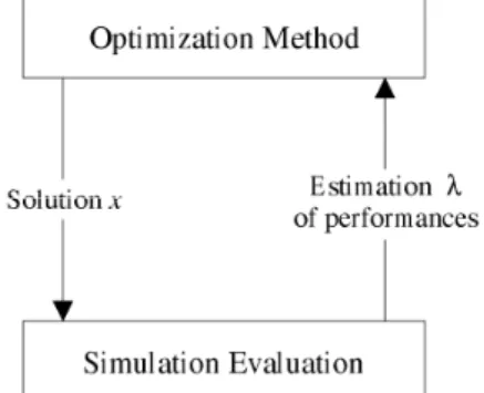
Cs represents constraints on a solution x. It usually defines the basic structure of a feasible solution (e.g. the route of the

bus must be a cycle in a graph representing the streets of the city). λ is a vector of measures (e.g. the travel times of the customers) that is returned by the simulation for a solution x (cf. Figure 1).

Λs(x) is the set of feasible solutions for λ, according to a given solution x. It is defined by implicit constraints of the

simulation model (given a solution x, the simulation returns the estimation λ), and by explicit constraints on some performance measures (e.g. the travel time of the customers must not exceed a given limit). That means Λs(x) contains

either one solution (x is feasible based on the simulation evaluation), or no solution (x is not feasible based on the simulation evaluation).

Figure 1: Simulation optimization sketch.

The objective function fr of the real problem is approximated by fs. We propose to parameterize this function on vector λ:

fs(x) = g(x,λ). For instance, λ can represent estimated times of travel for solution x, and g(x,λ) an estimation of the

satisfaction of the customers for solution x according to these times.

Simulation optimization explores the set of solutions Cs to optimize fs. For each solution x, the simulation estimates vector

λ. If λ satisfies all the constraints in Λs(x), the solution x is accepted, and the objective function g(x,λ) is evaluated.

Several methods are proposed to solve problem (Ps). A classification in four major approaches can be found in [Merkuryev

and Visipkov 1994] and [Azadivar 1992]: gradient based search, stochastic approximation, response surface and heuristic search. These methods are robust to changes in the objective function or in the constraints of the problem. However, they only represent a few optimization techniques and their efficiency and convergence are not always ensured.

(4)

3. Straightforward Optimization

Optimization techniques, independent of simulation, usually need a mathematical model (Po). This representation is also

an approximation of the real problem (Pr).

However, we can reasonably assume that the simulation optimization problem (Ps) is closer to the real problem than the

straightforward optimization problem (Po): in our example, the optimization model (Po) assumes that there is no waiting

time at the bus stops, contrary to the simulation model (Ps) that inherently takes this data into account. For the purpose of

model enhancement, we now make some assumptions on the structure of (Po).

• The constraints Cs describe the basic structure of a feasible solution. Hence, we can reasonably assume that the

constraints defining Co are approximations, and even relaxations, of the constraints defining Cs. It means that

Co⊃ Cs. For instance, Cs can force a bus route to be an elementary directed cycle (i.e. without any loop), thus

simulation optimization will explore the space of solutions more easily; whereas Co can allow any kind of

directed cycle, the space of solutions will be bigger, but straightforward optimization will solve the problem more easily.

• We consider that the objective functions fo and fs are identical: fo(x) = g(x,λ). However, we assume that the space

of solutions Λo is an approximation of the space of solutions Λs, which implicitly makes fo an approximation of fs.

In our example, Λs(x) will be a statistical estimation of the travel times of the customers, whereas Λo(x) will be a

deterministic computation.

Depending on the structure of the problem, various optimization techniques can be considered to solve (Po). However,

once a particular method m has been chosen to solve the problem, it is difficult to deal with changes on the kind of constraints of the problem. For model enhancement purpose, we consider changes only on the constraints that describe Λo.

Let us denote Km the set of all the families of constraints that can be managed by method m. That means problem (Po) is

solvable by method m only if Λo∈ Km.

4. Model Enhancement

From the previous assumptions, if Λo(x) is never empty, all solutions x ∈ Co are feasible solutions of problem (Po). As

Co⊃ Cs, any solution of the simulation optimization problem (Ps) is a feasible solution of (Po). In particular, any optimal

solution xs* of (Ps) is a feasible solution of (Po). The idea of model enhancement is to find the family of constraints

Λo∈ Km such that the optimal solution xo* of (Po) is one of the optimal solutions xs* of (Ps). We can state the model

enhancement problem (Pe) as follows.

(Pe) is a very hard problem. However, one way to find a good solution to the problem may be to approximate Λs by Λo as

precisely as possible. Thus, λs and λo* will have similar values and the theoretical evaluation g(xo*,λo*) of the optimal

solution xo* of problem (Po) will be close to its simulation evaluation g(xo*,λs).

This approach is inspired by decomposition methods like Benders’ decomposition or the column generation [Lasdon 1970], which propose to decompose a problem into two parts: the relaxed master problem, which is a relaxation of the original problem and the auxiliary problem, whose resolution provides useful information to enhance the relaxed master problem. Through an iterative process, the resolution of auxiliary problems will allow to add constraints or variables (depending on the decomposition approach) into the relaxed master problem, which will tend progressively to the original problem, and will provide an exact optimal solution.

(5)

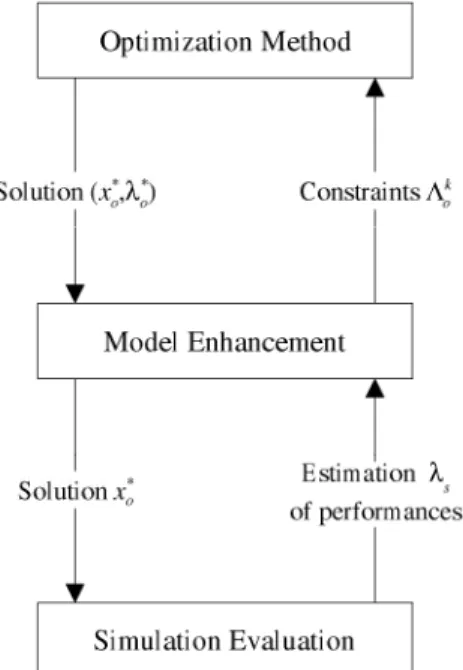
We can propose a similar decomposition for model enhancement: (Po) is the relaxed master problem, and simulation

experiments act like resolutions of auxiliary problems that provide information to enhance the relaxed master problem. In our example, (Po) does not consider waiting times at bus stops. The evaluation λs of its optimal solution xo* using

simulation provides estimations of these waiting times. Based on this information, we need to find a way to modify Λo so it

better approximates Λs.

Figure 2: Model enhancement heuristic.

Algorithm 1 and Figure 2 describe a heuristic approach for model enhancement that iteratively modifies Λo, based on the

simulation evaluation λs of an optimal solution of (Po).

Algorithm 1: Model enhancement heuristic.

k ← 0;

let n be the maximal number of iterations; let Λok be an approximation of Λs;

repeat

let (xo*,λo*) be an optimal solution of (Po) with Λo = Λok; letλs be the simulation evaluation of xo*;

Λok+1 ← h(Λok,λs); k ← k+1;

until | g(xo*,λo*) - g(xo*,λs) | < ε or k ≥ n;

Function h represents the way to modify Λo at each iteration. It needs to be defined more precisely for any specific

problem. In the next section, we propose to illustrate this heuristic with more details on the bus routing problem we mildly use as example in the first part of the article.

5. Study of a Routing Problem

We propose now to study a bus routing problem in order to illustrate the discussion of the previous sections. We detail the simulation optimization method, a straightforward optimization approach and the model enhancement heuristic for this problem. We also present a practical comparison of these three approaches.

5.1. Problem Presentation

We focus on the following problem: let us consider a public transportation company in an urban network, such as a bus company. Basically, this company needs to design low cost bus routes while satisfying potential customers.

(6)

Let us consider a directed graph G = (V,E) where V is the set of vertexes and E the set of edges. Each vertex represents a potential bus stop or a crossroad in the real-life network. Each edge represents a road between two stops or crossroads. We assume the customer demands are known, i.e. there is a description of the moves the customers need to perform in the urban network. A customer demand d ∈ D is defined by a tuple (od;sd;Qd;tdmin;tdmax), where od∈ V is the origin of the

move, sd∈ V the destination, Qd the throughput of customers for this demand. td min

and td max

are reference times for the demand: tdmin is the time it takes to a vehicle (such as a bus) to move from od to sd; and tdmax is the time of travel of a

pedestrian from od to sd.

In this article, we limit the problem to find a transportation system Γ that meets the following requirements: • Γ is a set of directed cycles in graph G (for clarity reasons, we consider further only one bus cycle);

• the length of the bus route, i.e. the time it takes to the bus to move along the route, must be less than a given threshold T;

• Γ should maximize the satisfaction of the customers.

Let us denote td the time it takes to a customer with demand d to travel through the network. His satisfaction can be

represented by a function Φd(td) defined as follows: if td≤ 2td min

then the customer is fully satisfied and Φd(td) = 1; if

td≥ 2tdmax then the customer is not satisfied at all and Φd(td) = 0; and between these two limits, the closer to the minimum,

the better the customer is satisfied. Figure 3 illustrates the satisfaction function.

Figure 3: Satisfaction function for demand d.

Finally, we define wi the time customers are waiting at a bus stop i. Back to our notations of the previous sections, λ is the

vector of all the td and the wi values. λo will be their theoretical estimation (from optimization) and λs their practical

estimation (from simulation).

Let us denote x a solution to the problem, i.e. xe = 1 if edge e is part of the bus route, and xe = 0 otherwise. The objective is

to maximize the satisfaction of the customers, i.e. function g(x,λ) = Σd∈D QdΦd(td).

5.2. Simulation Optimization

We propose to solve the problem using the tabu search metaheuristic in the simulation optimization sketch (Ps). The tabu

search was first introduced by [Glover and Laguna 1997] and [Herz et al. 1997]. It searches for a good solution x in the space of solutions Cs. Cs represents bus routes with their length below T. Moreover, we force the structure of the bus routes

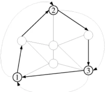
in Cs to be a geodesic (the search is thus facilitated). A geodesic is a directed cycle defined by a given number of points

called control points. Each control point is connected to its successor in the cycle by a shortest path (cf. Figure 4).

(7)

Neighborhood structures for the heuristic rely on moving, adding or deleting a control point. The tabu list contains the control points that have been modified in the last few iterations. We have implemented a two-level heuristic using aspiration criteria (accepting a tabu move under some conditions) and diversification strategy (exploring another area of the space of solutions).

For a given solution x of the simulation optimization problem (Ps), simulation estimates the time of travel td of the

customers with demand d and their waiting time wi at bus stop i (reminder: all these values are stored in vector λ). Besides

the implicit constraints of simulation, we consider no additional constraints in Λs that can discard a solution x based on its

estimation λ. That means any solution x ∈ Cs is a feasible solution of (Ps) (it is a necessary condition for model

enhancement to work).

Discrete-event simulation is used to simulate the system, i.e. the bus and the customers are individual entities, whose moves are simulated to estimate the waiting times at the bus stops and the travel times of the customers (in order to evaluate their satisfaction).

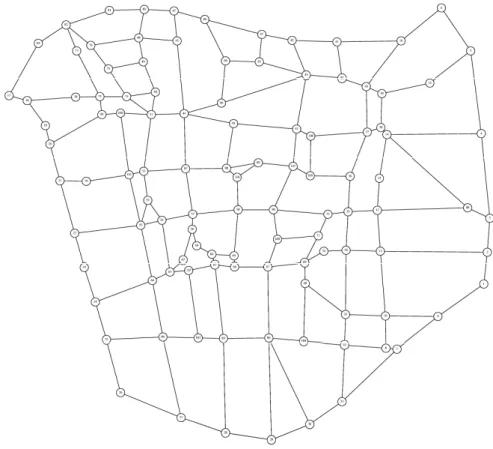
Figure 5: Graph modeling Clermont-Ferrand (France) downtown.

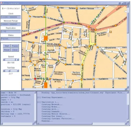
We consider now a graph with 109 vertexes and 392 edges that represents Clermont-Ferrand downtown (cf. Figure 5), with 12 customer demands. Table 1 presents numerical results for the simulation optimization on this instance. In order to test various problem structures, the number of control points in a geodesic varies. We also consider several maximal lengths T for the bus route. The tabu search has been implemented with C++ and the simulation model with the B++ Simulator framework 1 (cf. Figure 6). The tests have been performed on a Pentium Centrino 1.7 GHz with G++ 3.2 compiler.

1

(8)

Figure 6: Visual representation of the simulation.

Execution times can be more than a day. As our purpose here is only to know good practical solutions to compare with model enhancement's ones, we choose to limit the number of diversifications. Notice that the number of simulation evaluations to solve (Ps) is high, and without our restriction, it can reach more than 100000 evaluations. Hence, the

solutions provided here are not always the best ones that simulation optimization can provide.

(9)

5.3. Straightforward Optimization

Our bus routing problem is strongly related to the well-known Vehicle Routing Problem (VRP) class. Several straightforward optimization techniques can be considered to solve the problem [Toth and Vigo 2002]. Especially, [Yon et

al. 2003] propose a mixed integer programming formulation. They show that the tabu search (as defined in the previous

section) can provide solutions very close to the optimal solution (when known) or to the best known solution (when it takes to much time or memory to get an optimal solution using mixed integer programming).

Thus, we prefer to choose the tabu search as our method m to solve the optimization problem (Po). It still searches a good

solution x, but this time in the space of solutions Co. With mixed integer programming, Co would be larger than Cs

(Co⊃ Cs), because instead of forcing the solution to be a geodesic, it would look for any directed cycle. With tabu search,

it is easier to keep the geodesic structure, so Co = Cs.

Λo is an approximation of Λs. The implicit constraints of simulation that define Λs are replaced by constraints to estimate

the time of travel td of the customers with demand d. Other constraints fix the waiting times wi to zero for any bus stop i,

due to the assumption that there will be enough buses on the bus route for the waiting times to be insignificant. To sum up, Λo approximates the way to estimate the travel times and sets the waiting times to zero.

Table 2: Straightforward optimization numerical results.

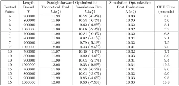
Under the same conditions than problem (Ps), tests have been performed for (Po). The problem is solved with tabu search.

Table 2 shows the theoretical evaluation fo(xo*) of the best solutions xo* found for (Po), and their simulation evaluation

fs(xo*). The resolution is quite fast (around 10 seconds) compared to simulation optimization (several hours), but the

solutions do not always have good simulation evaluations. Inside parenthesis is indicated the relative difference ( fs(xo*) -

fs(xs*) ) / fs(xs*).

5.4. Model Enhancement

Simulation optimization provides good practical solutions, but needs a very long time to execute (cf. Table 4). At the opposite, straightforward optimization is very fast, but provides poor practical solutions. We describe now the model enhancement heuristic (as proposed in Section 4) applied to our bus routing problem, in order to improve the contraints defining Λo so problem (Po) provides good practical solutions.

In problem (Po), we assumed that the waiting times wi are set to zero at any bus stop i. These constraints may make Λo a

poor approximation of Λs. As the method used to solve (Po) can deal with any constant waiting times wi ≠ 0, we propose to

modify these theoretical waiting times at each iteration of model enhancement (in order to make Λo a better approximation

of Λs).

Let us denote wik the waiting times for problem (Po) at iteration k, and λs = (w t), composed of vectors w = (wi)i∈V (the

estimated waiting times) and t = (td)d∈D (the estimated travel times), the simulation evaluation of the current theoretical

solution xo*. If wi≠ 0, that means i was effectively used as a bus stop during the simulation. Thus, we propose to tend wik+1

to wi as follows: wi k+1_← wi k + ∆(wi - wi k

). If wi = 0, that means i is a vertex where customers never stop. However, we

propose to tend wik+1 to the mean M of the waiting times (estimated since the start of the algorithm) as follows: wik+1←

(10)

∆ < 1 is a progression step that needs to be tuned. One can choose ∆ either constant, or variable according to the number of iterations (in order to ensure some convergence). For this routing problem, we choose a constant ∆ = 0.1 and decide to

stop the model enhancement after n = 100 iterations, or when there is some convergence, i.e. the difference between the theoretical evaluation fo(xo*) = g(xo*,λo*) and the simulation evaluation fs(xo*) = g(xo*,λs) is less than ε = 0.01. Algorithm 2

summarizes the model enhancement heuristic for our bus routing problem. Algorithm 2: Model enhancement heuristic for bus routing problem.

k ← 0;

for each vertex i ∈ V do wik ← 0; repeat

k ← k+1;

solve (Po) with waiting times wik, i ∈ V; let (xo*,λo*) be an optimal solution of (Po); letλs = (w t) be the simulation evaluation of xo*; update mean M of the estimated waiting times; for each vertex i ∈ V do

if wi≠ 0 then wi k+1 _← wi k + ∆(wi - wi k ); else wik+1 ← wik + ∆(M - wik); end for; until | g(xo*,λo*) - g(xo*,λs) | < ε or k ≥ n;

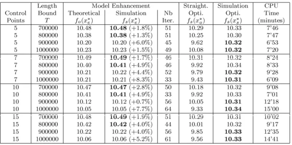
Under the same conditions than problems (Ps) and (Po), tests have been performed for model enhancement. Table 3

indicates the theoretical evaluation of the best solutions xe* found. It shows that it is very close to the simulation evaluation

of the same solution. In parenthesis, it indicates the relative improvement of the practical quality of the solution compared to straightforward optimization: ( fs(xe*) - fo(xo*) ) / fs(xo*). The number of iterations of the model enhancement process is

also provided.

Table 3: Model enhancement numerical results.

The resolution is slower than straightforward optimization, but is really faster that simulation optimization (cf. Table 4). In fact, few calls to simulation evaluation are required, contrary to simulation optimization that needs a large amount of evaluations. The quality of the solution provided by model enhancement is usually close to the one provided by simulation optimization, and always improves the solution provided by straightforward optimization.

(11)

Table 4: Execution times comparison.

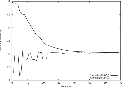
Figure 7 shows the evolution and the convergence of both theoretical and simulation evaluations of solution xo* at each

iteration k of the model enhancement process, for the search of a 10-points geodesic with T = 1000000. At the beginning, the theoretical evaluation is far from the simulation one, it is due to the fact that all the waiting times are considered to be zero in the theoretical model. Progressively, the waiting times information is injected into the theoretical model, which makes the theoretical optimization to provide various optimal solutions (that are not always very good in practice, which explains the variations in the first iterations). Finally, a good solution is found, with its theoretical evaluation very close to the simulation one.

Figure 7: Solution estimation evolution with model enhancement, case 1.

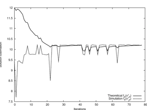
The convergence seems to be achieved quite easily in this case. However, Figure 8 shows the same kind of evolution for the search of a 7-points geodesic with T = 1000000. As shown in this figure, the heuristic sometimes oscillates between several good solutions, thus the convergence is more difficult to achieve.

(12)

Figure 8: Solution estimation evolution with model enhancement, case 2.

6. Conclusion

Simulation optimization provides good practical solutions. However, it may take a long time to execute, with lots of simulation evaluations. At the opposite, for some problems, like the routing problem presented here, efficient theoretical approaches can efficiently solve simplified formulations. But, usually, they find solutions that are not so good in practice. We propose in this article an approach called model enhancement that still focuses on the theoretical problem, and tries to improve its formulation in order to take into account practical aspects (estimated by simulation). The final goal is for the theoretical approach to provide good practical solutions.

We formalize model enhancement as problem (Pe) which, in some conditions, should provide the best practical solution

(according to simulation evaluation). This problem seems actually very hard to solve. It proposes nevertheless a different way to think of optimization and simulation coupling. Therefore, we present a quite simple heuristic for model enhancement, illustrated on a routing problem. Experimental results show the potential of model enhancement, which needs further investigation.

ACKNOWLEDGMENTS

We would like to thank Antoine Mahul, PhD Student at Blaise Pascal University, Clermont-Ferrand, France, for his invaluable advice to formalize model enhancement.

REFERENCES

[Azadivar 1992] F. Azadivar. A Tutorial on Simulation Optimization. Proceedings of the Winter Simulation Conference, pages 198-204, 1992.

[Glover and Laguna 1997] F. Glover and M. Laguna. Tabu Search. Kluwer Academic Publishers, 1997.

[Herz et al. 1997] A. Herz, E. Taillard, and D. de Werra. Tabu Search. Local Search in Combinatorial Optimization, pages 121-136. Princeton University Press, 1997.

[Hochbaum 1997] D. S. Hochbaum. Approximation Algorithms for NP-Hard Problems. PWS Publishing Company, 1997.

[Lasdon 1970] L. S. Lasdon. Optimization Theory for Large Systems. MacMillan, 1970.

[Merkuryev and Visipkov 1994] Y. A. Merkuryev and V. K. Visipkov. A Survey of Optimization Methods in Discrete Systems Simulation. Proceedings of the First Joint Conference of International Simulation Societies, pages 104-110, 1994.

(13)

[Nemhauser and Wolsey 1999] G. L. Nemhauser and L. A. Wolsey. Integer and Combinatorial Optimization. Wiley-Interscience, 1999.

[Toth and Vigo 2002] P. Toth and D. Vigo. The Vehicle Routing Problem. SIAM Monographs on Discrete Mathematics and Applications, 2002.

[Yon et al. 2003] L. Yon, A. Quilliot, and C. Duhamel. Distance Minimization in Public Transportation Networks with Elastic Demands: Exact Model and Approached Methods. Information Processing: Recent Mathematical Advances in

Optimization and Control. Mathematical Sciences and Computing series. Presses de l’Ecole des mines de Paris, pages