Damage resistance and damage tolerance of thin composite facesheet honeycomb panels

Damage Resistance and Damage Tolerance of Thin Composite Facesheet Honeycomb Panels

by

Simon Charles Lie

S.B., Massachusetts Institute of Technology (1987)

Submitted in partial fulfillment of the requirements for the

degree of

MASTER OF SCIENCE IN AERONAUTICS AND ASTRONAUTICS

at the

MASSACHUSETTS INSTITIUTE OF TECHNOLOGY March 1989

© Massachusetts Institute of Technology 1989

Signature of Author

Certified by

Department of Aeronautics and Astronautics March 2, 1989

//- rofessor James W. Mar . /,I ./ Thesis Supervisor Accepted by

S/Professor Harold Y. Wachman

Chairman, Depaetak-.&ire-edate Committee

JUN 07 1989

Aero

LUeIRMIES NITHDRAwIN

SM.I.T.

LIBRARIES

Abstract

Damage Resistance and Damage Tolerance of Thin Composite Facesheet Honeycomb Panels

by

Simon Charles Lie

Submitted to the Department of Aeronautics and Astronautics on March 2, 1989 in partial fulfilment of the requirements

for the Degree of Master of Science

An experimental and analytical investigation was made into the behavior of sandwich panels with two- and three-ply woven fabric graphite/epoxy facesheets subjected to low-velocity impacts. The facesheets were made from

AW193PW/3501-6, a plain wave fabric made from Hercules AS4 fibers and 3501-6 epoxy. The core material was 3.0 pcf Nomex. Damage was observed to begin at an energy level of

1.0 ft lbs. Damage consisted of core crushing, matrix cracking, fiber breakage, and delaminations. Panels were also subjected to static indentation which produced damage indistinguishable from impact damage. Damaged panels were then tested in compression to failure. Panels with (±45)

facesheets were found to be notch-insensitive and failed by local facesheet buckling (also called "facesheet wrinkling") at a constant value of net-section stress. Panels with

(0,90) facesheets were notch-sensitive and failed in the same manner at a lower value of net-section stress. Analytical models of the impact event and and compression test are able to predict the amount of damage caused and the residual

strength of the damaged panel. These models comprise a fast, preliminary analysis tool for use in design of sandwich

panels.

Thesis Supervisor: James W. Mar

Title: J.C. Hunsaker Professor of Aerospace Education

Acknowledgements

This document represents the work of many individuals. I would like to acknowledge some of many people who made this project possible. Thanks to Darrin Tebon and Sen-Hao Lai for the design and construction of the heavy parts of FRED.

Thanks to Al Supple, who taught me many useful things, such as the ins and outs of three-phase wiring. Thanks to Ping Lee, who rarely fails us though we expect her to know

everything. Thanks to all the graduate students, especially Kevin Saeger, Pierre Minguet, and Wilson Tsang for providing

insight, encouragement, and a little sanity. Thanks to Professors Dugundji, Graves, and Lagace for their thoughts and guidance. Special thanks especially to Professor James Mar for his supervision, encouragement, and the freedom with which he allowed me to tackle this project.

And lastly, a very special thanks to three individuals whose assistance has been indispensable. They are

responsible for the majority of the work as well as the moral of the team: Krista Beed, chief scriber; Dave Fleming, chief aligner and illustrator; and Rich Pemberton (the one with the short hair), chief data taker and doughnut maker.

This thesis is dedicated to Edie'Erlanson and those from Camp Cebuano, whose support and encouragement has made this possible.

Foreword

This work was conducted at the Technology Laboratory for Advanced Composites (TELAC) in the Department of Aeronautics and Astronautics at the Massachusetts Institute of

Technology. The work was sponsored by Boeing Helicopters under purchase order number TT 964237. The project monitor was Steve Llorente.

Table of Contents List of Figures • .... .. . •. •. ... ... .. .. .. ... ...7 List of Tables ... List of Symbols ... 1. Introduction ... 2. Theoretical Analysis ... 2.1 Background... 2.2 Analytical Approach... 2.3 Global Model... 2.4 Newmark Integration... 2.5 Local Model... 2.6 Hertzian Spring Constant 2.7 Failure Criteria... 2.8 Damage Predictions ... 2.9 Residual Strength Model. 3. Computer Implementation .... 4. Experimental Procedures .... 4.1 Test Objectives... 4.2 Manufacturing Procedures 4.3 Testing Procedure... 5. Results ... 5.1 Global Model Performance 5.2 Local Model Performance. 5.3 Material Properties...

5.4 Damage Types - Two-Ply Facesheets... ...91

Table of Contents ... ... ... ... ... •.. ... ... ... ... Determinat 4. 06. -. . . . . .. .. .. . o• .. . . . . . . . . . .. ... o...oo... ... ... oo.. oooe... .oo.oo... .. oeooo.e... ... .oo... ... . . . ... ... ... ... ... ion ... ... ... ... ... ... ... ... ...

5.5 Damage Types - Three-Ply Facesheet Specimens...93

5.6 Static Indentation Damage ... 94

5.7 Force-Time History...94

5.8 Force-Indentation Relation ... 97

5.9 Damage Quantitation...100

5.10 Residual Strength - Undamaged Panels...105

5.11 Residual Strength - Damaged Panels ... 108

6. Conclusions ... 114

References ... 118

Appendix A: FORTRAN Source Code ... 119

Appendix B: Analytical Results ... 213

Appendix C: Experimental Data ... 216

List of Figures

Figure 2.1 Analysis Overview ... 18

Figure 2.2 Modeling Method ... 19

Figure 2.3 Global Model Panel Geometry ... 20

Figure 2.4 Impact Geometry ...36

Figure 2.5 Newmark Integration Scheme ... 38

Figure 2.6 Plate on an Elastic Foundation ... 43

Figure 2.7 Compressive Strength Modeling ... 51

Figure 2.8 Mar-Lin Relation with Corrections ... 57

Figure 3.1 Computer Model Overview ... 60

Figure 4.5 Laminate Cure Layup ... 70

Figure 4.6 Laminate Cure Temperature History ... 71

Figure 4.7 Laminate Cure Pressure History ... 71

Figure 4.8 Laminate Cure Vacuum History ... 72

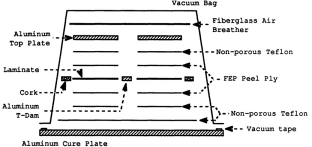
Figure 4.9 Panel Cure Assembly ... 74

Figure 4.10 Panel Cure Temperature History ... 74

Figure 4.11 Panel Cure Pressure History ... 75

Figure 4.12 Test Specimens ... 76

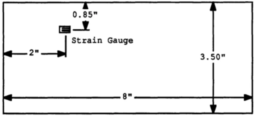
Figure 4.13 Strain Gauge Locations ... 77

Figure 4.14 Specimen Holding Jig ... 79

Figure 4.15 Impactor ... 80

Figure 4.16 Anti-Rebound Lever ... 81

Figure 4.17 FRED - Striker Unit ... 82

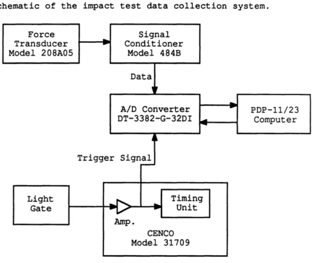
Figure 4.18 Impact Test Data Collection System ... 83

Figure 4.19 Static Indentation Apparatus ... 84

Figure Figure Figure Figure Figure Figure Figure Figure Figure 5.1 5.2 5.3 5.5 5.6 5.7 5.8 5.10 5.11 Figure 5.12 Figure Figure Figure Figure Figure Figure Figure Figure Figure 5.13 5.14

5.15

5.16 5.17 5.19 5.20 5.21 5.22 Figure 5.23 Figure 5.24 Figure 5.25

Global Model Convergence (Me Global Model Convergence (Tj

Local Model Energy Balance

)des) ... .me Step) ..

...

Core Crushing ... Fiber Breakage Pattern ...

Force-Time History - 1.32 ft lb Impact Force-Time History - 1.49 ft lb Impact Experimental and Analytical ... Force-Indentation Curve

0.09 inch Indentation ... Force-Indentation Curve

0.12 inch Indentation ... X-ray of a Damaged Specimen ... Predicted Strain Contours ... Damage Extent and Damage Prediction .. Damage Width vs Impact Energy ... Damage Width vs Indentation ... Compression Test - zero load ... Compression Test - 2760 lbs ... Compression Test - post failure ... Failure Stress versus Damage Width

(0,90) Specimens... Failure Stress versus Damage Width

(±45) Specimens ... Failure Stress versus Impact Energy

(0,90) Specimens ... Failure Stress versus Impact Energy

(±45) Specimens ... i List of Figures

....

...

88

... 89 ... 90 ... 92 ... ... 93 ... 95 ... 96

... 98

... 99 ... 99 ... 101 ... 102 ... 103 ... 104 ... 105 ... 109 ... 109 ... 110 ... 111 ... 112 ... 113 ... 113

List of Tables

Table 3.1 Program Execution Times ... 63

Table 4.1 Test Matrix SO ... 65

Table 4.2 Test Matrix S1 ... 66

Table 4.3 Test Matrix S2 ... 67

Table 4.4 Test Matrix S3 ... 68

Table 5.4 Material Properties ... 91

Table 5.9 Experimental Curve-Fit Parameters ... 97

Table 5.18 Undamaged Panel Strengths ... 106

Table B.1 Analytical Results for (0,90) Specimens ... 214

Table B.2 Analytical Results for (±45) Specimens ... 215

Table C.1 Data From Test Matrix SO ..; ... 217

Table C.2 Data From Test Matrix S1-L ... 218

Table C.3 Data From Test Matrix Sl-M ... 219

Table C.4 Data From Test Matrix S1-N ... 220

Table C.5 Data From Test Matrix S2-L ... ...221

Table C.6 Data From Test Matrix S2-M ... 222

Table C.7 Data From Test Matrix S2-N ...223

Table C.8 Data From Test Matrix S3 ... 224

List of Symbols

a panel length A,B constants

A.. components of the laminate extensional stiffness matrix

[A] laminate extensional stiffness matrix b panel width

B_i buckling load for mode shape i (residual strength model)

d damage width

d₁,d₂ change over points in the corrected Mar-Lin relation (residual strength model)

D plate bending stiffness E modulus of elasticity

E.. components of the material stiffness matrix EL longitudinal modulus

E transverse modulus

[E] material stiffness matrix EI _{bending stiffness of the beam} F contact force acting on the panel F _max maximum contact force

F tensile strength

G _{local minimum of strain energy at fixed value of X} GLT shear modulus

h core thickness

H_c composite fracture toughness i,j dummy variables

I area moment of inertia k Hertzian spring constant

[K] panel stiffness matrix

m number of modes in the x-direction (global model)

mo impactor mass [M] panel mass matrix

n number of modes in the y-direction (global model) Snumber of modes (residual strength model)

N1,N 2 linear shape functions

p,q dummy variables P applied load Pcr buckling load

qkij time-varying generalized coordinates (global model) qkij time-varying generalized velocities (global model) qkij time-varying generalized accelerations (global

model)

qi generalized coordinates (local model)

generalized coordinates (residual strength model) {q} _{vector of generalized coordinates (global model)} {q} vector of generalized velocities (global model)

{q} vector of generalized accelerations (global model) r,s dummy variables

E distance from impact point

Qi'Qkij normalized modal forces (global model) {Qi) vectors of modal forces (global model) ta thickness of facesheet A

tb thickness of facesheet B

T kinetic energy of the panel (global model)

Ua, va, w a ua Va' Wa ub, vb, wb

ub' Vb' Wb

U C Vcf _W V v

w

0 Wext

{w}

x, y, z za z_ac zb Zbc

a

max At 8.. cult

Oi

Cartesian displacements of facesheet A Cartesian displacements of facesheet A Cartesian velocity of facesheet B

Cartesian velocity of facesheet B Cartesian velocity of the core Cartesian velocity of the core

potential energy of the panel (global model) velocity vector

displacement of the impact site on the panel external work done on the panel by the impactor column of values of mode shapes evaluated at the

impact site

Cartesian coordinates

z coordinate of the center of facesheet A

z coordinate of the core-facesheet A interface z coordinate of the center of facesheet B z coordinate of the core-facesheet B interface indentation

maximum indentation

exponent in force-indentation relation time step interval

Kronecker delta strains

failure strain

Euler beam function mode shapes satisfying the x-direction boundary conditions (global model)

mode shape (local model)

beam function mode shape integrals (x-directions)

K modulus of foundation (local model) / beam length

Sshape parameter

VLT Poisson's ratio 7E 3.14159...

fi total potential energy of the system (residual strength model)

p volume density

G_o buckling stress - undamaged specimen Ocr buckling stress - damaged specimen

CO areal density

t,(,ý non-dimensional Cartesian coordinates

Vj Euler beam function mode shapes satisfying the y-direction boundary conditions (global model)

Y beam function mode shape integrals (y-directions)

1. Introduction

In recent years, advanced composite structures have become the subject of investigation for use in aerospace

structures. In particular, sandwich structures have shown promise for use in rotary-wing craft.' The relatively low

static strength requirements coupled with stringent vibration (stiffness) requirements tend to favor light-weight honeycomb sandwich construction. In addition to strength and stiffness requirements, the structure must be able to withstand

accidental impacts and foreign-object damage. Currently, there is no consistent methodology for the impact analysis of honeycomb sandwich structures. This project is an attempt to develop a consistent methodology to predict the damage

resistance2 and damage tolerance3 of thin gauge composite honeycomb structures. Specifically, the goal is to

analytically predict the residual compressive strength of an impacted sandwich panel.

The project consisted of two portions: an experimental investigation and analytic modeling. As both portions were conducted simultaneously, insight from the experiments helped

1

The first all-composite helicopter, the Boeing Model 360, flew in June 1987.

2

Damage resistance refers to the amount and type of damage caused

by a specific impact event.

3

Damage tolerance refers to the residual strength of a damaged structure.

shape the analysis and preliminary analytical results helped determine the experimental parameters.

The information in this report is organized as follows: Chapter 2 contains the theoretical analysis; Chapter 3

describes the computer implementation of the analysis; Chapter 4 describes the procedures used to manufacture and test the sandwich structures; Chapter 5 contains the results of both the analytic and experimental portions of the

investigation; and Chapter 6 contains the conclusions and summary. FORTRAN source code listings and experimental and analytic data is contained in the three appendices.

2. Theoretical Analysis

2.1 Background

Many investigators have developed models of impact events. Cairns4 at MIT and Graves and Koontz5 _{at Boeing} Advanced Systems have each developed models. Cairns

developed a time-marching solution to the general problem of an impact to a laminated plate. Graves and Koontz developed a closed-form solution for the problem of an impact of an elastic body on a simply-supported or clamped orthotropic plate. Like Cairns' analysis, the present analysis is a time-marching method, but it is restricted to orthotropic sandwich structures with "thin" facesheets. These

assumptions allow simplifications which reduce the computational effort required for a solution.

Like Cairns', the present analysis treats the issues of damage tolerance and damage resistance separately and

independently. Each step in the analysis is a self-contained module which requires certain well-defined inputs and

produces specific outputs. With this type of architecture,

4

Douglas S. Cairns, Impact and Post-Impact Response of

Graphite/Epoxy and Kevlar/Epoxy Structures, Ph.D. Thesis, Massachusetts Institute of Technology, Department of Aeronautics and Astronautics,

August 1987. 5

Michael J. Graves and Jan Koontz, Initiation and Extent of Impact Damage in Graphite/Epoxy and Graphite/PEEK Composites, AIAA 88-2327,

Proceedings of the 29th Structures, Structural Dynamics, and Materials

Conference, Williamsburg, VA, 1988, page 967.

one step in the analysis may be easily changed or upgraded without modification to the remaining processes.

Before describing the analysis, a note about

nomenclature is required. The term "panel" shall be used to refer to a structure consisting of two facesheets bonded to a Nomex core. The terms "plate" and "beam" are used in the classical, abstract sense to refer to concepts used in the development of the model of the panel.

2.2 Analytical Approach

The present analysis addresses the problem of modeling a low-velocity impact of an object and a thin facesheet

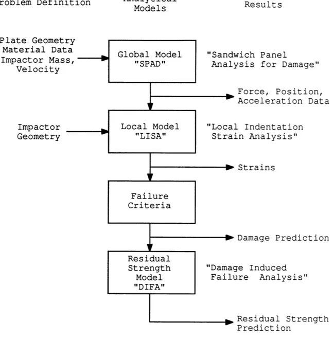
composite honeycomb sandwich panel. The analysis begins with an overall model of the impact event. The actual event is an interaction of two deformable bodies. Idealized models of the impact event will be formulated in sufficient detail to model the important physical aspects of the impact event. Figure 2.1, Analysis Overview, shows the flow of information through the different modules of the analysis.

Problem Definition Analytical Models PaLte Geomet: Material Dat Impactor Mas Velocity Impactor Geometry Results wich Panel

ysis for Damage"

Force, Position, Acceleration Data 1 Indentation in Analysis" Strains Damage Prediction ge Induced ure Analysis" Residual Strength Prediction

Figure 2.1 Analysis Overview

The impact event will be separated into two distinct models for analysis. The first model is an overall

examination of the dynamics of the panel and impactor called the "global model." The specific global model developed

here is known as "SPAD" - Sandwich Panel Analysis for Damage.

Theoretical Analysis

The results of the global model are used as input to the

second model. This second model is a detailed examination of the local strains near the impact point and is thus called the "local model." The specific local model developed here is known as "LISA" - Local Indentation Strain Analysis.

Together, the global and local models represent two separate physical phenomena: overall plate deflections and local deformations. Overall plate deflections are considered only in the global model. Local deformations are modeled by a Hertzian spring in the global model. In the local model, an energy method is used to analyze the local deformations. The following diagram is a graphical representation of the

relationship between the two models and the actual impact event.

U

Impactor

Panel

The Event Deformed Panel

Global Model Local Model

Figure 2.2 Modeling Method

2.3 Global Model

Let us now examine the global model. The geometry of the panel and impactor for the global model is defined as follows: z'FC Face A Cta Core h Z=Z Z=ac - z=0 Face B t_b x Y z a b h/2

Figure 2.3 Global Model Panel Geometry

Any engineering model begins with assumptions and idealizations. The following assumptions are used for the formulation of the global model:

1. _{The sandwich panel is rectangular in shape and is} composed of two uniform orthotropic facesheets perfectly bonded to a uniform thickness core.

2. _{The facesheets are thin relative to the core so that} under bending, the stresses are assumed constant through the thickness of an individual facesheet

(plane stress).

3. The core is "soft" in that its stiffness in the x-y plane is negligibly small compared to that of the

facesheets.

4. The panel is ideally supported by any combination of free, simply-supported, or clamped conditions which prevent rigid body translation and rotation. Neither

adjoining nor opposite sides are required to have the same boundary conditions.

5. The impactor is assumed to be rigid compared to the panel.

6. The strains in the panel will be small, that is to say, describable by linear strain-displacements relations.

7. Both the facesheets and the core are assumed to obey linear stress-strain relations.

8. The impact is assumed to follow the Hertzian Contact Law6 for elastic bodies.

The problem is to find the displacements, and thus the strains, caused by an impact to the panel.

6

S.p. Timoshenko and J.N. Goodier, Theory of Elastic Stability, Third Edition, McGraw-Hill, Inc., Singapore, 1982, page 409.

The displacements of the panel are modeled by 6

independent quantities: ua, Va, Wa, Ub' Vb, and Wb7. These represent the displacements of the two facesheets, A and B respectively. The core displacements are interpolated

linearly from the facesheet displacements. Note that in this formulation, phenomena such as facesheet wrinkling and core crushing can be represented because the facesheets can deform independently.

In order to find a solution to this problem, the problem must be transformed from a continuous one to a discrete one.

In this formulation, the displacements will be represented as a finite series of modes which are separable in time and

space. These modes will be products of generalized beam functions8'9 in the x and y directions which satisfy the specified boundary conditions. The beam functions shall be designated by Oi(4) and j () . For brevity, the functional dependence will not be shown; q is a function of time only,

4

is a function of 4 only, and A is a function of 11 only. Let m and n denote the number of modes in the x and y directions

7

Here and elsewhere, the subscripts a, b, and c refer to facesheet A, facesheet B, and the core, respectively.

8

John Dugundji, Simple Expressions for Higher Vibration Modes of Uniform Euler Beams, Technical Note, AIAA Journal, Volume 26, No. 8, August 1988, page 1013.

9_Note:

These beam functions do not exactly satisfy the boundary conditions. The worst error occurs in the lowest mode and is

approximately 0.5% of the maximum amplitude.

respectively. There need not be the same number of modes in each direction. Also, because the facesheets are

orthotropic, there is no bending-twisting coupling. A centerline impact will excite only symmetric modes and thus the anti-symmetric modes need not be included in the

analysis.

The displacements are written: m n Wa =I Yqii _j

i=j=1

_(la) m n ua i Yq 2ijz a ₁ j i=1 j=1 m n Va= ~I ,3qijza i i=1 j=1 m n

b

_{i=1 j=1}

4 i j

m n

U = _ijzbo' i=1 j=1 m n bi=1 j= 6ij b (Ib) (Ic) (Id) (le) (If)

where: #i and yj are generalized beam functions which satisfy the prescribed boundary conditions, qkij are generalized displacements representing modal amplitudes,

and the prime notation denotes spatial partial differentiation.

In the modal amplitudes qkij; k varies from 1-6 referring

to wa , a a wb , Ub, or vb respectively; i varies from 1 to m referring to the x direction mode number; and j varies from

1 to n referring to the y direction mode number.

Note that the displacements u and v, i.e., the in-plane mode shapes, are composed of w, i.e., the out-of-plane mode shapes. These in-plane modes where chosen so that the model could correctly represent pure bending of thin plates with no shear deformation. Under Kirchoff assumptions of thin plates

with no mid-plane extension, the out-of-plane displacements imply certain in-plane displacements. These displacements

are given by:

aw

u =- z•x (2a)

aw

v=-z

- Zy _(2b)

The right-hand-sides of the these equations were chosen to serve as the in-plane displacement modes. The negative

sign was omitted from the mode shapes and becomes

incorporated into the modal amplitude. If the six modal

amplitudes, qkij, are equal'l for all modes (i.e. q sij=qt for s,t in {1..6}) then the displacement field represents pure

10_{Due to the inclusion of the negative sign in the amplitudes of} the in-plane modes, the actual condition is qlij = -q2ij = -q3ij"

bending which satisfies the Kirchoff assumptions of no mid-plane extension and no shear deformation.

The core displacements are interpolated linearly from the facesheet displacements as follows:

w =N w +N w c 1 a 2 b _(3a) u =N u +N _c u 1 a 2 b (3b) v =N v +N v c ₁ a ₂ b _(3C)

where the shape functions N₁ and N₂ are defined as:

1 1

N=1+()+0

_{1 2}

N=

1a-0

2 2 (4a,b)

where: _{h z} h/2

Substituting the expressions for the facesheet

displacements (equations la-1f) into the above equations gives the core displacements in terms of the modal

amplitudes:

m n

wc 1 lij+2 4 i

i=1 j1 _(5a)

m n

c _{i=1 j=}1 (N2ij ac+N2 5ijbc j

(5b)

m n

V= Z E(Nl 3ijzac+N ₂q 6ijbc)O i

i=1 j=1 _(5c)

The modal amplitudes qkij are the generalized coordinates of the problem. With this formulation, as many modes as

desired may be used, but generally 3 or 4 in each direction is sufficient. The number of generalized coordinates is the number of unknowns and is equal to (6 x m x n).

Because the facesheets are assumed to be thin relative to the panel, each facesheet is assumed to be in a state of plane stress. Thus, all quantities are assumed constant through the thickness of each facesheet. Also, the core material (Nomex) is very soft in the x and y directions relative to the facesheets and thus its stiffness in these directions is assumed to be zero. With these assumptions, the interesting strains in the panel are ₁,' E₂, and E6 in the facesheets and C3V ' 4, and F5 in the core. Because the overall

strains in the panel are expected to be small, linear strain-displacement relations are used to write:

In the facesheets:

au

1 ax _(6a)

8v

2 ay _(6b)

au

av

6--•y + 6 y x _(6c) In the core: aw 3 8z _(7a) aw av 4 ay _{8z (7b)} Theoretical Analysis__

aw u

5 =x +z _(7c)

Note: Engineering rather than tensor shear strain is used.

Substituting the expressions for the displacements

(equations 1 and 5) into the expressions for the the strains

(equations 6 and 7) gives expressions for the strains in

terms of the modal amplitudes _qkij:

In face A:

m n

, = I q z ao"iv

1 i=1 j=1 2ij _(8a)

m n 2 q 3ijZa 2 i=1 j=1 3ij i _(8b) m n 6 = 1 (q 2ijq _{j)z a} i=lj=1 2ij 3 _(8c) In face B: m n I=

X

jq z 0"

1 _{i=1j=1 5ij b j (9a)}

m n 2 - q6ijb 2 i=1 j=1ij b _(9b)

=m

(q

+q )zb

'i

6 5ij 6ij. b i=1 j=1 _(9c) In the core: m n 3 ij 4ij i(a)

i=1 j=1

_(10a)

Theoretical Analysis

m n

4 = (Nlij -N24ij 1 3ij ac 6ij jz i

m n

5==

(N

qlij- N24ij +

ijac

5 ijzbc1

i=1 j=1

(10b)

(10c)

The equations of motion of the panel are found using Lagrange's Equations":

d (aT aT _av

dt .I(+ i F

dt

Y

)

aq. Dq -F I

S1 1 ₍₁₁₎

where: T is the kinetic energy of the panel, V is the potential energy of the panel, F is a scalar representing the total force applied to the panel,

and Qi are normalized modal forces associated with the generalized displacements qi"

Our goal, then, is to express the kinetic and potential energy of the panel in terms of the generalized

displacements. With this in mind, let us begin.

Potential Energy

The potential energy of the panel is given by:

V= f{ eT _{[E]{ d d dz}

panel ₍₁₂₎

11

Raymond L. Bisplinghoff and Holt Ashley, Principles of Aeroelasticity, Dover Publications, Inc., New York, 1962, page 35.

Breaking this integral into separate regions

the facesheets and core gives:

v= L Jff{E a}

T

_{[E {a} d dy dz}

face A +

JE

f bf

E

b dx dy

dz

face B

+

f f f • c

}[E

c]{c}dx

dy

dz

core where: 1 6

1[

{b} = [3 c8 c (14a,b,c) and [E

a]

E 11 E 12

0

E 0 12 E 0 22 0 E

66

(15a) E 11

[E-

b]

_E12

o

[E

c]

[

E 0 12 E 0 OE 66 E33 0 0 33 0

0

E

0

0

0

E

55 Theoretical Analysis (13) (15b)

(15c)

___ · covering

The assumption of plane stress within each facesheet allows us to use classical laminated plate theory12 to write:

n

ply [

[A=

f[Eldz=

_pl

_y

i=1

(16)

Thus, equation 13 becomes:

V= _{{a} Aa]{ a}dx dy}e

face A

+

2 II

eb bT

b dxdy

face B

+ L ff T [Ec cdy ecldx dz

core (17)

Substituting equations 14 and 15 into 17 yields:

1 2 2 2

V

fJ

(AE

+2A

E PE

+A

E

+A

)E

dc

dy

2 11 1 12 1 2 222 66 face A +- (A e2 +2A E E +A +AE ) dx dy 2 11 1 12 1 2 222 666 face B +- f 355(E , 2 +E e2 +E , 2 )dxdy dz 21 333 3 44 4 555) dy dz core

(18)

By substituting the expressions for the strains in terms of generalized displacements into this equation, we have the desired expression for potential energy in terms of

generalized displacements. For brevity, we will show only

12

Robert M. Jones, Mechanics of Composite Materials, Scripta Book

Company, Washington, DC, 1975, page 154.

the first of the 15 individual terms of the resulting equation (the example term is due to Alla)

1 -m n a Am M n[ fce "

V=

2

All

q2ij

z a f

_.da

_q2rsZa

_Vs

_{da +...}

i=1 j=1 faceA r=l1 s=1 face A

(19)

Note that the only x or y dependency in the equation is contained in the # and A terms. The integrals of these terms over the panel can be taken separately and are written as:

( (i,j,p,q) = - d1

t=0-L a -t (20a)

T (i,j,p,q) =

dTI

)b02(

where: i and j are dummy variables signifying mode shape

number,

and p and q are dummy variables indicating which derivative of the mode shape is to be used.

Substituting for the integrals in equation 19, we have:

V= 1 abA z2 1 q .q 4 (i,r,2,2) ~Y(j,s, 0,0) +

2 11 a 21i 2rs

i=l j=l r=- s= (21)

This procedure produces all 15 terms for the potential energy V. Note that all terms are quadratic in qkij. When the partial differentiation called for by Lagrange's Equation

(equation 10) is performed, these terms become linear in qkij" Rewriting these equations in matrix notation results in:

where [K] is a 6mn by

1

mnl

Iq2mn}

Iq3mnI

Iq4mnI

Iq5mn} q6mn . 6mn matrix. Energy

The kinetic energy due to the motion of the panel is given by:

T=21 ffp( o)dx dy dz

panel

where: v is the vector velocity,

(23)

and p is the material density.

Again, we break this integral into separate regions:

T

IIIff

(pa+P

face A

+1

ff

(

+p

face B (v 0) dx dy dz (v* v) dx dy dz

+

fffpc(v.

) dxdydz

core (24)

where pf represents the density of the film adhesive bonding the facesheet to the core.

The dot product v* v may be written as:

Theoretical Analysis

Kinetic

(22)

.2 .2 .2

*Ov=

_{(u +v +w )}

₍₂₅₎

Also, the assumption of plane stress within the

facesheets allows us to perform the z direction integration separately as:

fpdz= (26)

(26) where CO is the areal density.

Substituting equations 25 and 26 into equation 24 yields:

1

.2 .2 .2

T= 2 (Coa+ f)O (U+ va + Wa) dx dy

face A 1 r.2 .2 .2 + ₂ (J (u a+o + )(( _b +v +w )dx dy f b b b face B 1 frr 2 *2 *2 +*

jp

(c

c+Vc+ w dxdy dz core ₍₂₇₎

In the expressions for u, v, and w (equations 3a-f), the only time-dependency is the qkij terms. By differentiating the expressions for the displacements with respect to time, we obtain the expressions for the velocities:

m n a= 1 qlij ivj i=lj-1 _(28a) m n ua= I Iq2ijzb _{i j} i=1 j=1 _(28b) m n a = I 1q3ijzaiI _ij i=1 j=1 (28c) Theoretical Analysis_ _

m n b 41 i j i=Ij=1 _(28d) m n u = q z b',Yi b _{i=1 j=1} 5ij bXj (28e) m n vb = iq 6 z i' i=1 j=1 _(28f)

These expressions may be substituted directly into equation 27. _{As with the potential energy, the integrals of 0 and IV} are replace by (D and y (equations 20a-b). Again, for

brevity, only the first term is shown:

T= ab(pa+p) ₍(9ijql q rsq((i,r, 0, 0 (n,s, 0,0)) + i=l j=1 r=l1 s=1l

(29) These terms are all quadratic in qkij (the generalized velocities). _{The differentiation with respect to the}

qkij called for by Lagrange's Equations produces terms linear in qkij. The time differentiation then produces terms linear in qkij" Using matrix notation, the kinetic energy may be

written:

d

_dtOki

i -=

[MI.

j {q ii {q2ij

q3ij

4ij {q 5ij q6ij1 1 \ X-"JI Theoretical Analysis

Generalized Forces

Because the impact force is assumed to act only in the z direction with no surface shears, the generalized forces Qi are defined as:

{0}o

F{Q}=F. (0)

{o}

{(0

(31)

in which the only non-zero components are:

{Q

₁ij=

J

P(x,

y)

i

jdxdy

face A (32)

where: pz(x,y) represents the normalized force distribution produced by the impact event. Note: pZ has units of in-2 .

As this integration is done numerically, any shape may be chosen for the function pZ. The only restriction is that the force distribution be normalized such that:

I pz(x,y) dxdy= 1

panel ₍₃₃₎

For this study, a square load patch is used with total area equal to the area of the impactor. Within this load patch, the load is assumed constant.

The equations of motion of the panel are now complete.

Impactor

The equation of motion of the impactor is given by: m0q0=-F

(34) where: m₀ is the mass of the impactor,

q0 is the position of the impactor, and F is the force applied to the panel.

Additionally, we have the Hertzian contact law which couples the two sets of equations.

F

=

ka

2

₍₃₅₎

where: F is the contact force,

a is the approach (see Figure 2.4), and k is the Hertzian spring constant.

Figure 2.4 Impact Geometry

Theoretical Analysis 36

From Figure 2.4, it can be seen that the approach a may be written as q0-w0. Expressing w0 in generalized coordinates gives:

m n T

i=1

j=1

₍₃₆₎

so that the contact law (equation 35) may be written as:

mn 3/2

3/2

F = ka3/2 =k iq·~ 0j _{iq (}

(

i=1

j=1

3

₍₃₇₎

or, in matrix notation:

T 3/2 F =k(q - {W} {q}

0

₍₃₈₎

We now have the following equations:

The equations of motion of the panel, in matrix form,

[M] {q} + [K]{q}= F {Q} ₍₃₉₎

the equation of motion of the impactor,

m0 _{0 -} F

(40)

and non-linear contact law which couples the motion of the panel and impactor (equation 38).

2.4 Newmark Integration

The equations of motion are ordinary differential equations in time and are solved by the Newmark constant

average acceleration scheme13. In this time-marching scheme, the acceleration is considered constant over the interval of one time step. For each acceleration, the value used is the average of the values at the beginning and end of the

interval. The velocity is then calculated using this assumed value of acceleration. The position is calculated similarly

from the velocity. The following diagram represents the scheme: Acceleration • Velocity Average

q

j+1

q

Average

q

j+l

Figure 2.5 Newmark Integration Scheme

Mathematically:

j+1

+At(

+

₍₄₁₎₎

q

=q

+-2

q

+qI

₍₄₂₎

where: qJ denotes the quantity q at time step j.

By eliminating qj+l from these equations and solving for

q j+l we have:

13_{K.J. Bathe, Numerical Methods in Finite Element Analysis,}

Prentice-Hall, Inc., New Jersey, 1982, page 511.

-.000

t

a

4 -

A

t

q 2\, q - q iAt

At (43)

substituting (43) back into (42) gives:

Sj+1

2 j+1

Ij J

S=

~At

₍₄₄₎

Note that in this equation there are still quantities at the current time step as well as at the previous time step on the right-hand-side.

By substituting the new expression for the acceleration (equation 41) into equation 37, we can write the equation of motion of the panel at time step j+1.

[M

4q

- q -

t - q + [K] {q

+=

F

j+1 Q

(45)

solving for qj+l yields:

q j+= [_42[M] + [K]] _SAt F J+{Q} + [M] q J+ _At 4 (qj + JAt ₍₄₆₎

We can also write the contact law (equation 38) at time j+1: 3/2

j+1 1 jAt 2 F T 3+1

F

=k

q

+At o+

4

0

m

{

S0 0 ₍₄₇₎

We now have two equations (46 and 47) for two unknowns (qj+l and Fj+1). Substituting equation 46 into equation 47 yields:

Theoretical Analysis 39

SFj+3/2

j 2 j+1 j+ q0 +AtqFAtq + - q F =k ClOl-1i·,,,~ [W 4 [M ] + [K]] {F F {j+1 2(qj

At

At

(48)

This equation is now of the form:

3/2

F = k(AF + B) (49)

with the following definitions for the scalars A and B:

2 -1 A = 40 EAt (50) 2 __ -1

B=

q

+i+

At

+

At

W}T

4

_{[M]+ [K]}

₊

₊

0 0)

At

2

_At

(51)

We now have all the required equations to implement the solution. The procedure at each time step is as follows:

1. Form the quantities A and B (equations 50 and 51). 2. Solve equation 49 for Fj + l . _{Newton-Raphson iteration}

is used for this procedure. If the quantity (AF+B) in equation 49 is less than zero, the panel and impactor are no longer in contact and the force is set to zero. 3. Calculate qj+l (equation 46). 4. Calculate qJ+l (equation 44). 5. Calculate qj+l (equation 43). j+1 6. Calculate q₀ (equation 40). 7. Calculate qJ+l (equation 41). Theoretical Analysis

8. Calculate q j+1 (equation 42).

This completes the calculation cycle. The time marching scheme is continued until two conditions are met:

1) The impactor loses contact with the panel, and 2) The impactor has rebounded past its original

position.

In this way, the complete global response of the panel can be found. From the analysis, any desired quantities can be extracted, such as force-time history, position-time

history, maximum deflections, maximum impact force, etc.

2.5 Local Model

From the global model, the point of maximum indentation (which is also the point of maximum force) is singled out for further study in the local model. The maximum indentation and maximum force are denoted max and F respectively. The local indentation problem is a static problem in which the back surface of the panel (facesheet B) remains fixed and an

indentation of amax is imposed at the center of the top of the panel (facesheet A).

Castigliano's theory of least work states that the correct stress state is the one which minimizes elastic

strain energy.14 We shall then seek the stress/strain state which minimizes the elastic strain energy of the panel.

As with the global model, the displacements of the panel are modeled by 6 independent unknowns (wa, Ua' Va, Wb, Ub, and vb). However, because we assume that facesheet B remains fixed, three of the displacements are immediately constrained to be zero. The remaining displacements are modeled by a single assumed mode separable in time and space as follows:

Wa=q1 ) ('n _(52a)

Ua 2(t) aax _(52b)

a

a 3(t) aay (52c)

where: P(~r1) is the mode shape

and gi(t) are the generalized coordinates.

As with the global model, this choice of mode shapes allows the Kirchoff no-shear bending condition to be

satisfied for thin plates. Note that in the local model, a single assumed mode shape is used to model the displacements.

14

Robert M. Rivello, Theory and Analysis of Flight Structures, McGraw-Hill, New York, 1969, page 120.

Mode Shape

Timoshenko solved a related problem in which an isotropic plate supported by an elastic foundation is subjected to a out-of-plane line load. The plate is considered to be infinitely long and of unit width.

Isotropic Line Load Plate

y

x

Elastic Foundation

Figure 2.6 Plate on an Elastic Foundation

The plate is loaded at x=O by a line load of P/unit width. Timoshenko shows that the deflections of the plate are given as15:

w(x=-e cos x+ sin -1x

2jk

=2

%2

(53

where: 4 = K/D is the shape parameter,

K is the modulus of the foundation expressed as pressure exerted/unit deflection,

15

S. P. Timoshenko and S. Woinowsky-Krieger, Theory of Plates and

Shells, McGraw-Hill Book Company, Inc., New York, 1959, page 253.

and D is the plate bending stiffness.

Although this problem is not the same as ours, it can be considered similar. The top facesheet acts very much like a plate on an elastic foundation (the core). Therefore, we can expect the form of deflections in the local indentation

problem to be similar to equation 53. Timoshenko's solution is for a line load, but our problem is a point load. If the facesheet and core were isotropic, then the indentation

problem would be exactly axisymmetric. Although the facesheets and core are orthotropic, we shall assume an axisymmetric mode shape derived from equation 51. By

rotating the above solution about the z-axis, the following axisymmetric mode shape is formed:

(4,) = e-(J)[cos (XJ) + sin (?X)] (54) where:

X

is the shape parameter,

2 2

and r = __) _ + _

The shape parameter, X, will be left as an unknown in the problem. The total number of unknowns is now 4: three generalized displacements (qi) and the shape parameter (X).

The strains are formed from the displacements by using strain-displacement relations. In the facesheets, non-linear terms are included to account for the high strains near the impact region. In facesheet A:

au

[u

]2[2

a

2

_2+wl

1= + L + L-Jx I] (55a)

yav

v

1

•rul rv rw

2

[

_{]2+,2 ]2]}

=av +

ax ay

av av

aw aw

6- ax ay ax ay ax ay ax ay (55b)

(55c)

In the core: aw 3 DZ

aw

av

4-

y

Dz

8 u aw E z + ax 5-

az

ax

(56a) (56b)

(56c)

The strain energy, U, is given by:

S[E]{8} dv

plate ₍₅₇₎

The formulation of the strain energy is similar to the formulation of the potential energy described earlier. The

only difference is that non-linear terms are included in the expressions for the strains. The resulting expression for strain energy is a function of 4 unknowns: l,' q2' q3, and ?.

The condition that the displacement of facesheet A match the indentation found using the global model imposes an

additional constraint on the problem. Specifically,

1A = . =

(2 2 2 2 max ₍₅₈₎

However, the value of the mode shape at the center of the plate (4=0.5, 11=0.5) is independent of the shape parameter h and is equal to 1. Thus, the indentation constraint can be written:

q₁ max

(59)

This removes one degree-of-freedom from the model. The strain energy U is now a function of 3 variables. At this point, the values of q1, q2' and X which minimize the strain energy must be found.

The calculation of the strain energy is much less

involved if X is held constant. Thus, the fewer times X is varied, the faster the calculation will proceed. To take advantage of this characteristic, the function U is rewritten as follows:

U = G(X) (60)

where: G(1) is the minimum value of U(X,q•11 2) at fixed

Note: a two-dimensional minimization occurs for each evaluation of G(X).

The two-dimensional minimization (over -q and 42) _is

done using the Downhill Simplex Method16. The one-dimensional minimization over X is done using Brent's Method17 which

combines bisection and parabola fitting. The result of this process is the value of the shape parameter and the

generalized coordinates.

At this point, the entire local displacement field can be determined. As the global displacement field has already been determined, the total displacements can be found by summing the results from the local and global models. The total displacements are given by:

In Facesheet A:

m n

a ij i 4 1

i=lj= _(61a)

m n d

U aq= I _{2ijZa i( j (T+ 2z adx(,}

i= j=1 _(61b)

16_{William H. Press, Brian P. Flannery, Saul A. Teukolsky, and}

William T. Vetterling, Numerical Recipes - The Art of Scientific

Comuting, Cambridge University Press, Cambridge, 1986, page 289.

17

Press et al, page 284.

m n

i=1j=1 _(61c)

With the displacements known, the strains can be

determined from the non-linear strain-displacement relations (equations 52 and 53). This portion of the analysis is now complete. From the properties of the panel and dynamics of the impactor, we have determined the strain field. This information is then be used for damage predictions.

2.6 Hertzian Spring Constant Determination

The local model can also be used to determine the value of the Hertzian spring constant, k, in the following

expression:

F = ka3/ 2 ₍₆₂₎

This equation can be written more generally as:

F=ka (63)

where:

P

is a free parameter.

Note: For the Hertzian contact law, the parameter

f

is

equal to 3/2.

Integrating both sides of equation 63 over the depth of the indentation yields an expression for the work done by the impactor: max max 1 ( +1) Wext ( F d = _{ka da - (+1) kamax} 0 0 (64) Theoretical Analysis

where: Wext is the work done on the panel by the impactor.

Note: In the local model, no global panel deformations are considered, so Wext represents only the work done during the local deformation.

The external work is stored in the panel as strain energy and this quantity is already calculated by the local model. Several values of the strain energy (external work)

are calculated - each for a different value of the

indentation. The constants k and 3 are then found by a two-parameter least squares analysis. In general,

P

will not be equal to the Hertzian value of 3/2. Nevertheless, the value of 3/2 is used in the analysis. This is done for two

reasons. First, the value 3/2 is theoretically justified; and second, the value of k is very sensitive to small

variations in P.

WIth

1

fixed to a value of 3/2, equation 63 becomes a equivalent to the Hertzian contact law, equation 62. A second least squares analysis is done to find the

corresponding value of k. This value of k is in general, different from the value found when

f

is a free parameter. This procedure can be done before the global model is run and thus the value of k determined can be used in the global model.

2.7 Failure Criteria

The purpose of finding the strain field caused by an impact event is to predict the amount and type of damage caused in the sandwich panel. Once the strains are

determined, several failure criteria are available to predict the occurrence of damage. For this study, a simple point-strain criteria is used. This criteria states that failure

(damage) occurs at any point at which the strain exceeds a specified critical value. Different strains cause different types of damage. In-plane extensional strains can be

expected to cause fiber breakage. In-plane shear strains can be expected to cause matrix cracks. Out-of-plane extensional and shear strains are expected to cause delaminations.

However, due to the assumption of plane stress, no out-of-plane information is generated and thus no predictions of delamination are possible.

2.8 Damage Predictions

For each strain in the impacted facesheet, a contour plot is made. On this plot, the contour corresponding to the failure strain serves as an outline of the predicted damage area. Different outlines are produces for different strains corresponding to different types of damage.

At this point, it should be noted that while the analysis method described here is used to predict damage,

both the global and local models assume that the panel remains undamaged throughout the impact event. A more

complete analysis would update the properties of the panel as soon as damage is predicted in any area, but such an analysis is beyond the scope of this investigation.

2.9 Residual Strength Model

Once the damage area is known, the next step is to predict the residual strength. However, first we must

analytically determine the undamaged strength of the panels.

The analytical failure loads are derived from the

following model: the sandwich panel is modeled as a beam on an elastic foundation with the facesheet and film adhesive together acting as the beam and the core acting as the elastic foundation. For this specimen configuration, the film adhesive with embedded Nomex contributes a significant amount to the bending stiffness of the facesheet.

Consequently, this effect must be included.

P

z,w

Beam

r~-~mr

8

x

Elastic Foundation

Figure 2.7 Compressive Strength Modeling

We shall assume that the beam is simply-supported at each end. This assumption will be justified later. Also, we shall assume that the mid-plane of the sandwich panel does not deform and that the failure mode is buckling of the beam. This phenomena is also known as "facesheet wrinkling."

The bending stiffness of the beam and modulus of the foundation are assumed to be constant. We shall use the principle of the stationary value of the total potential energy:

Of all compatible states of deformation of an elastic body, the true deformations (those which satisfy

equilibrium) are the ones for which the total potential energy has a stationary value for any virtual

displacement.18

To implement this principle, we shall use the Rayleigh-Ritz method19 _{of assumed modes. The displacements w are} modeled as:

S nnx w= Iqg sin

i=1 ₍₆₅₎

where: - is the total number of modes,

qi are the model amplitude (and thus generalized displacements),

/ is the length of the beam,

and x is the coordinate along the beam.

18

Rivello, page 118. 19Rivello, page 123.

Note: _{These modes satisfy the geometric boundary} conditions.

The total potential energy of the system is given by:

n = Ubending + Uspring / (2

EI

dw

2 f

0

( dx 2

- Wexternal (66) dx +

_2-0

IKw 2dx-

_2x

_{0 d x}

P d 0 0o ₍₆₇₎

where: K is the modulus of foundation, P is the applied end load,

and EI is the bending stiffness of the beam.

Substituting the assumed modes (equation 65) into the potential energy expression (equation 67) yields:

n n

2

2

1 -IJ i[ sin ix ~

l-

j s jsx

I= 1E qi q2 si - qj sin dx

01 i=1 j=1 l x j

+2q

'i=1 j=1

sin q sin- dxdx

1 n i i7x j7I

jnx

-

P oi

₁ i

sin -

q

j-

₇

sin

dx

oli=1 j=1

₍₆₈₎

Due to orthogonality of modes, only those terms with i=j are non-zero:

Theoretical Analysis

S _{2 4 2} S= ElJ .i 2 s in i dx Oi=. /

1 f

2

2 icxx

2--__ q sin dx 1 n 2

2ll Jo~

{/

sin , dx

0i ₍₆₉₎

Performing the integrals over the length of the beam yields:

,4 4 22

H= EI +--P

3 4 4 i

V= ₍₇₀₎

The virtual displacements are, in this case, the assumed modes themselves. For the total potential energy to remain stationary for these displacements requires that:

an

4 4 I4 .2

- TE i + 1-i -/2q. =0

qj i=l1

4

/3

4E

4

13

₍₇₁₎

where: 8.. is the Kronecker Delta:₁₃ =f1 if i=

j

ij 0 if i

j

The summation can now be eliminated. Rewriting equation 71 produces:

n

2( __i2 4

an-

=I i + =0

aqi

/

2

EI4

(72)

This equation is of the form:

(B.-P)4, = 0 1 1 ₍₇₃₎ where: B =EI 2i + / i EI4 In matrix notation: B1--P 0 ... 0 qO 0 B -P i }|J

0

0 ... O B -P

L R fi

₍₇₄₎

This equation will only have non-trivial solutions if the determinant of the diagonal matrix is zero. This gives:

(B - P)(B - P) ...(B - P)= 0

1 2 ₍₇₅₎

From equation 74, it can be seen that the mode which causes instability at the lowest load is the mode with the lowest associated value of Bi. This gives the buckling load:

I

E

El 2

KI/4

P cr = _{min EI}

2 4

/I E IIC (76)

where: Pcr is the buckling or facesheet wrinkling load.

We now have the failure load (or stress) for undamaged panels. For typical values of El and K, the mode with the

lowest buckling load is in the range of i=12 to i=20. For these short wavelength modes, the effects of end boundary

conditions (simply-supported, clamped, etc.) are negligible.

From equation 75, we know the failure load of undamaged panels. This load is converted to an equivalent stress and

is referred to as 00. This stress is used as a basis to predict the residual strength of a damaged panel. Two

separate methods are used to calculate the residual strength of a damaged panel: constant net-section stress (upper

bound) and the Mar-Lin relation2 0 _{(lower bound). If the panel}

is notch-insensitive, then the failure stress can be found by:

(b -d)

cr

O

d ₍₇₇₎

where: 0cr is the failure stress of the damaged panel, 00 is the failure stress of an undamaged panel, b is the panel width,

and d is the width of the damage area.

If the panel is notch-sensitive, then the Mar-Lin relation is used to predict the failure stress:

-0.28

cr =H (d) ₍₇₈₎

where: H_c is the experimentally determined composite "fracture toughness."

Note that as d approaches zero, equation 78 predicts that the failure stress will increase without bound. Also,

2 0

K.y. _{Lin, Fracture of Filamentary Composite Materials, Ph.D.}

Thesis, Massachusetts Institute of Technology, Department of Aeronautics and Astronautics, 1977.

as d approaches b, the predicted failure stress does not

approach zero. Thus, corrections must be made near d/b=O and near d/b=l. Consider a graph of equation with d/b as the abscissa and Ocr as the ordinate. A straight line is

constructed which passes through the point (d/b=O, Ycr=a0 ) and is tangent to the curve (equation 78). Let d_I denote the value of d at the point of tangency. Similarly, a second line is constructed which passes through the point (d/b=l, acr=0) and is also tangent to the curve21. Let d₂ denote the value of d at the new point of tangency. Figure 2.8 depicts the Mar-Lin curve and tangent lines.

2 1

Tangent line corrections are used by C. E. Federson in the study of cracked tension panels (metallic). C. E. Federson, Evaluation and Prediction of the Residual Strength of Center Cracked Tension Panels, ASTM Special Technical Publication 486, 1970, page 50.

Mar-Lin Relation with Tangent Corrections

0.0 0.1 0.2 0.3 0.4 Damage Width (d/w)

0.5

Figure 2.8 Mar-Lin Relation with Corrections

For values of d between zero and dj, the upper tangent line is used to predict the failure stress. For values between dI and d2, the Mar-Lin curve is used, and for values between d₂ and b, the lower tangent line is used. These

sections of the various curves appear as the dark line in Figure 2.8.

For all panels, the two methods (net-section and Mar-Lin) are used predict the upper and lower bound of the

residual strength. Panels with fibers perpendicular to the principal load axis are generally notch-sensitive and the

value of residual strength lies closer to the lower bound. Panels with fibers at 450 to the principal load axis tend to

be notch-insensitive and the residual strength approaches the upper bound.

Theoretical Analysis 59

3. Computer Implementation

The analyses described in Chapter 2 have been

implemented as FORTRAN programs on an IBM AT compatible computer. Microsoft's FORTRAN 4.1 Optimizing Compiler was used to compile the codes. Figure 3.1, Computer Model Overview, shows the different programs and associated data files. Problem Definition "filename." Figure 3.1 "filename." "filename.FRC" "filename.Q0" "filename.WA" "filename.WB" "filename.DIS" "filename.TQ" "filename.LSH" "filename.LQ" "filename.RS" filename.xxx "

Computer Model Overview