Data visualization of biological microscopy image analyses

Data Visualization of Biological Microscopy Image Analyses

Tony Scelfo

Submitted to the Department of Electrical Engineering and Computer Science in Partial Fulfillment of the Requirements for the Degrees of

Bachelor of Science in Computer Science and Engineering

and Master of Engineering in Electrical Engineering and Computer Science at the Massachusetts Institute of Technology

~May 26, 2006~

©2006 MASSACHUSETTS INSTITUTE OF TECHNOLOGY. All Rights Reserved.

The author hereby grants M.I.T. permission to reproduce and distribute publicly paper and electronic copies of this thesis

and to grant others the right to do so.

Signature of Author

Certified by

Accepted by

Department -f leeficalering and Comp er Science Ma 26, 2006

Peter Sorger Thesis Supervisor

L

Chairman, Department Committee

MASSACHUSETTS INSTflJT OF TECHNOLOGY

AUG

14

2006

BARKER

Data Visualization of Biological Microscopy Image Analyses

Tony Scelfo

Submitted to the Department of Electrical Engineering and Computer Science May 26, 2006

In Partial Fulfillment of the Requirements for the Degree of Bachelor of Science in Computer Science and Engineering

and Master of Engineering in Electrical Engineering and Computer Science

ABSTRACT

The Open Microscopy Environment (OME) provides biologists with a framework to store, analyze and manipulate large sets of image data. Current microscopes are capable of generating large numbers of images and when coupled with automated analysis routines, researchers are able to generate intractable sets of data. I have developed an extension to the OME toolkit, named the LoViewer, which allows researchers to quickly identify clusters of images based on relationships between analytically measured parameters. By identifying unique subsets of data, researchers are able to make use of the rest of the OME client software to view interesting images in high resolution, classify them into category groups and apply further analysis routines. The design of the LoViewer itself and its integration with the rest of the OME toolkit will be discussed in detail in body of this thesis.

Thesis Supervisor: Peter Sorger Title: Professor of Biology

Acknowledgments

The OME project is a joint effort between the Sorger Lab at MIT, the Wellcome Trust Biocentre at the University of Dundee in Dundee, Scotland, the Image Informatics and Computational Biology Unit at the National Institute of Health in Baltimore, and the Laboratory for Optical and Computational Instrumentation at the University of Wisconsin. I would like to thank everyone I have worked with at each location.

Specifically, I would like to thank the following individuals.

At the University of Dundee, I would like to thank Jean-Marie Burel and Chris Allan for helping me understand the inner workings of Shoola and the OME server. The work done in Dundee would never be possible without everything that Jason Swedlow has done to guide the project and motivate its development.

At MIT, outside of the Sorger Lab, I would like to thank Anne Carpenter for creating CellProfiler and helping me with any and every question I had about using it.

Within the Sorger Lab, I would like to thank Doug Creager and Jeff Mellen for getting me involved with the project, Erik Brauner and Jeremy Muhlich for providing excellent guidance, and Sheldon Chan for provided invaluable assistance at every step in the development of the LoViewer.

Finally, I would like to especially thank Peter Sorger for making it possible for me to be involved in the OME project though support by MIT CDP Grant #P-50-GM68762 and ICBP Grant #5-U54-CA1 12967-02.

Table of Contents

1 Introduction...9

1.1 O M E project...10

1.2 Project Evolution/Sum m ary... 11

1.3 D ata Scrubbing... 14

2 D ata Analysis...16

2.1 H and Annotation... 16

2.2 Scripted Analysis... 17

2.3 A utom ated Batch Processing... 19

3 The LoV iew er...22

3.1 The Shoola Client... 22

3.2 D ata V isualization... 23

3.2.1 Launching the LoV iew er... 24

3.2.2 V ariable Selection... 26

3.2.3 Region Selection... 28

3.2.4 Single A xis H istogram s... 31

3.2.5 D ata Point Selection... 33

3.3 Shoola Integration ... 36

4 D esign and Im plem entation... 38

4.1 LoV iew er Overview ... 40

4.2 LoV iew er as part of Shoola... 40

4.2.1 LoV iew er A gent w ithin Shoola... 41

4.2.2 M essage H andling... 41

4.2.3 Loading a Dataset/Image and Image/Feature data... 41

4.3 Core Classes...43

4.3.1 Plug-in Classes... 43

4.3.2 LoV iew er Class... 43

4.3.3 LoM anager Class... 44

4.3.4 V iew Port Class... 44

4.3.5 Classes for D ata Transport/H andling... 44

4.3.6 Classes for Draw ing to the Screen... 46

4.4 Event H andling, A ctions... 47

4.4.1 Plotting D ata... 47

4.4.2 Dragging Sliders... 47

4.4.3 Dragging Selection Box... 48

4.4.4 Panning and Zoom ing... 48

4.4.5 Tim e Slider... 48

4.4.6 A lternate Click... 49

5.1 Future Work ... 50

6Appendix A: ... 52

List of Figures

Figure 1: Shoola's data manager showing alternate click menu. The LoViewer menu item launches the LoViewer to visualize data for the selected image or dataset...25 Figure 2: Example of a LoViewer data plot. The selection window in the local analysis tab allows the user to choose which measurements to plot. The OME server tab contains the same selection window, but points to data on the OME server as opposed to the local data store. The number bars next to the plot show the range of data values and allow the user to define selection regions by dragging sliders... 27 Figure 3: This plot shows a selection window defined by sliders on the number bars. Data values that are shaded out are excluded from the selected region...29 Figure 4: LoViewer prevents a user from panning off of the data range by limiting a pan such that the corner of the data range lies in the center of the screen...30 Figure 5: LoViewer alternate click menu showing options that the user can select to change the zoom level... 31 Figure 6: Histogram shown in the number bars for a plot that is zoomed out...32 Figure 7: Histogram shown in the number bars for a plot that is zoomed in...32 Figure 8: LoViewer alternate click menu showing options that the user can select to highlight data points... 34 Figure 9: Data points are selected in a region of interest based on the relationship

betw een tw o plotted variables... 35 Figure 10: A previously defined selection is maintained when the data points are plotted

against different variables. Here we can see that the data points that were previously selected are evenly distributed across the image based on their X and Y position and that they do not correspond to the large cells in the image... 36 Figure 11: Block diagram of the LoViewer application overview. Each shaded region represents a logical grouping of classes. Some minor classes and numerous methods have been excluded to enhance the clarity of the diagram... 39

I

Introduction

Quantitative analysis of biological images is a common technique for learning about complex biological processes. Images are often the subjects of numerical analysis via simple and complex visual processing algorithms. With modern microscopic equipment, it is possible to capture still images and high-resolution movies of cells exposed to small molecules or RNAi oligos in experiments that explore thousands of targets at a time. Variation in cell behavior caused by RNAi and drugs allow researchers to test and verify complex biological models. In the past few years, the hardware and methods of running high-content experiments have become sophisticated and efficient. However, tools to store the raw image data, derived quantitative data and subsequent observations are substantially less developed.

As might be imagined, systematic storage solutions are few and far between. Frequently ad hoc methods of organizing data are used. For example, data is stored in custom spreadsheets, and observations are made in lab notebooks and tied to data via cryptic codes. Images are often inspected one at a time via simple file system browsing tools and programs geared to visualization rather than data management such as Metamorph'. Although ad hoc tools are capable of handling small and medium sized image sets generated by a single of user, their usefulness diminishes drastically when they are applied to large datasets or to data shared among multiple users.

1 MetaMorph, Universal Imaging Corporation.

One solution for this problem has been developed by a group of collaborators under the Open Microscopy Environment (OME) umbrella. OME is a set of tools that aim to close the loop between image capture, image analysis and meaningful conclusions. OME achieves this goal by providing a means to store both image data and image meta data via a universal and extensible data model. Meta data is defined as important information that is needed to fully understand an image's context. By providing a means to store a full log of data history and steps of analysis, data can be presented in the context of fully specified provenance.

1.1 OME project

The OME project is a joint effort between the Sorger Lab at MIT, the Wellcome Trust Biocentre at the University of Dundee in Dundee, Scotland, the Image Informatics and Computational Biology Unit at the National Institute of Health in Baltimore, and the Laboratory for Optical and Computational Instrumentation at the University of Wisconsin. Over the past several years, the OME team has produced a set of tools for the management and storage of biological images and data resulting from biological (and largely optical) microscopy. At the core of the OME project is a set of standards for representing meta data. The world of microscopy is composed of numerous microscope manufactures, researchers and different methods of sample production. Currently, when data is produced and stored, it is done in a proprietary way that is fully understood by one group of individuals or company. The OME standards allow that group to fully specify all of the parameters involved in data generation such that others can understand the context of a piece of data and its corresponding provenance. For example, the OME project has created an XML schema that is rapidly becoming the standard for microscope data export file formats.

Beyond the core standards, the OME team has also produced a set of tools that allow researchers to interact with their data. As soon as images are captured on microscopes, they can be imported into the OME server, which is comprised of an efficient file system

and a PostgreSQL database for storing image meta data. Several tools exist that interface with the OME server to allow users to browse their data and to perform analysis on images. In addition, a rich Java client has been built that interfaces with the OME server. This client, named Shoola, allows researchers to interact with their data in an environment that makes use of a client's (rather than a server's) computational power. For example, the Shoola client can be used to view high-resolution images in parallel with any notes and classification information that has been assigned to the images.

Whenever data is stored in the OME server or images are examined, a complete transaction history is maintained transparently. The server also allows analysis routines to be installed and launched against image sets. An analysis chain is defined in the server by specifying a chain of modules to execute on an image. When the chain is executed, the server records which analysis modules are run, what the inputs are, and what outputs are produced. Complete transaction history is essential for biological analysis where input parameters are often tweaked to produce the final results. Without the parameter values, the result is meaningless. In addition to input parameters, the analysis techniques themselves are often modified as new techniques for identifying morphological data from images are developed. By providing a framework to record complete data provenance, OME functions as much more than a complex image warehouse for massive quantities of images.

1.2 Project Evolution/Summary

A server/client architecture for OME was chosen when the project began. Labs often have available several powerful machines to function as servers in addition to a suite of client machines that live on researchers' bench tops. Given the typical layout of laboratory informatics equipment, the OME system was developed to take advantage of the computational power and storage capacity of massive servers. The idea of a server-side analysis chain provides means for powerful servers to handle many complex analysis routines. Furthermore, by conducting analysis on the OME server itself, the task of

persisting computational results and the steps taken to reach them is greatly simplified.

Recently, the MIT OME group began to explore alternative methods for conducting analysis and interacting with analytical data. Specifically, Sheldon Chan, another master's student in the group, and I have developed ways for researchers to rapidly conduct analysis and explore results on their local system. Our vision is that researchers will use OME as a tool for long term data persistence where complete data provenance is extremely important. In the short term, however, we feel that it is too awkward to upload analysis routines to the OME server and then trigger server-side analysis just to explore new variables or methods.

The idea of performing analysis outside of the OME server is extremely powerful given the unused computing power of most desktop systems. Chan has developed a tool that allows researchers to connect to a server, download images to a local scratch space and then batch process the images using local analysis routines.2

His external analysis tool is written as a component for the Java-based Shoola client. As a result, any analysis method that can be wrapped in Java can be interfaced with the OME server via his local analysis tool. Chan has also extended the Shoola client to support local data storage. When researchers explore new analysis routines, it is important that they have rapid access to data that need not persist with complete provenance. The local data storage component of Shoola provides researchers with a way to rapidly develop analysis routines locally and then choose sets or subsets of analysis results that need to be fully persisted in the OME server. When the analysis results are uploaded to OME, the local analysis component is careful to persist a complete history of what analysis was performed to ensure adherence to the OME data provenance model.

The local analysis work that Sheldon has done ties closely to the work I have performed on data visualization. High-content biological screens are able to generate hundreds of thousands of images. These images are processed to generate hundreds of millions of 2 A Modular Architecture for Client-Based Analysis of Biological Microscopy Images, Sheldon Chan

data points that correspond either to image wide measurements or to measurements of specific regions, or features in image. The goals of my work are to explore ways to visualize the resulting measurements in an efficient manner. The results of this work are described in section 1.3.

In addition to the changes we have explored in the Java client, developers at Dundee are exploring new server architectures. The link between the Java client and the server is currently made using an JAVA package built on top of XML-RPC. The OME-JAVA package allows the Java client to request objects from the server, such as a collection of all images that belong in a data set. This method works well for simple data structures, but does not perform well with the complicated hierarchical objects that are used to store data within the OME Java client. The current server architecture requires the following process for data retrieval through OME-JAVA: a request is made to the server, a set of Perl scripts read information from the PostgreSQL database and group the data into hierarchical structures, the data is then serialized for transmission over XML-RPC, and then finally the XML is interpreted by the Java client and hierarchical Java objects are created. This process is not very efficient and the performance of server/client communications falls rapidly when data sets contain hundreds of images, a not uncommon number for high-content analysis. The Dundee group's newly proposed server architecture, named OMERO, revolves around a Java-based server. The communications layer between the server and the client leverages high performance third party middleware applications for transporting Java objects from the server to the client. Initial tests have shown one hundred-fold speed increases for common server/client exchanges.

Based on the promising results of the Dundee group, we at MIT are committed to supporting the new server architecture in all of our Shoola client applications. However, OMERO is still immature and we are currently unable to test our applications directly against the new architecture. However, by ensuring that our applications use a single interface class for data exchange with the OME server, we ensure that applications that

work with the current version of OME can easily be modified to work with any future version of OMERO.

1.3 Data Scrubbing

My primary interest has been in the development of OME tools for high-content screening applications. My work has been to develop tools that help researchers view large quantities of analytical data and thereby identify subsets of images that might prove interesting. I use the phrase data scrubbing to describe the process by which users isolate subsets of images by sifting through large quantities of analytical data. This data comes in the form of numerical values that correspond to features and attributes within an image. To make sense of the massive amount of data generated by high-content biological screens, it is essential that individuals be able to scan rapidly through it. It is also a necessity to view analytic data generated through both server analysis chains and local analysis operations.

It is not uncommon for a single high-content screen (one part of an experiment) to generate tens of thousands of images and hundreds of millions of data points. It is not feasible to view all of the images from a single screen, let alone multiple screens within a single experiment. By using singular analytic descriptors of images, researchers can identify clusters of similar images as well as unique outliers to send to other OME tools for further analysis. In addition to whole images, analytic data can belong to regions, known as features, within the images. The most obvious instance of a feature for a biological image is a cell. In the context of high-content screening, automated analysis

algorithms have been created to identify cells and measure their morphologies.

Data scrubbing has proven itself to be one of the only interactive ways to identify which

images are interesting for further visual inspection. Due to the scale of data explosion caused by high-content experiments, the tools for researchers must be fast and efficient. Users must be able to quickly view the relationships between several analytic

measurements to discover which relationships lead to meaningful clusters and outliers. By identifying the analytic measurements that yield significant relationships, immense data sets can be approached efficiently. Furthermore, data scrubbing can provide researchers with a starting point for building automated classification models.

2 Data Analysis

Many different tools, mechanisms and algorithms exist for deriving analytic data from images. Some tools require interaction with the user while others are fully automated. The set of image analysis methods can be broken down into three main categories, hand annotation, scripted analysis and automated batch processing. I describe each method in the following subsections.

2.1 Hand Annotation

Some labs rely entirely on hand annotation. This means that the members of the lab collect images and then go through each image to look for key characteristics. For example, visual inspection is often required to identify which stage of the cell cycle is captured by an image or the age of a tissue sample. In these types of situations, labs are often looking to make observations based on a relatively small collection of high-resolution images. Often, the distinctive attributes and characteristics are too subtle to be

detected by a machine.

In the work flow of hand annotation, images are classified into a set of categories as they are inspected. After a set of images have been classified, a microscopist can ask questions about samples that belong to a certain category. An example of such a question would be seeing if a certain treatment leads to a common phenotype. In another application, researchers might want to pull up all of their images that correspond to a

certain stage in the cell cycle, such as mitosis, to then look for morphological differences between the samples.

Regardless of application, hand annotation is used in situations when there are sufficiently few images that they can all be given individual attention. In its current stage of development, the OME Java client provides an adequate set of tools for conducting hand annotation. These tools come in the form of a single image viewer and a classification tool that lets the user associate images with custom category groups.

2.2 Scripted Analysis

To approach data sets that are too large for hand annotation, labs often write scripts that perform analysis routines. The analysis scripts are often built on top of common

laboratory image analysis platforms such as Matlab3 and ImageJ4

. Both Matlab and ImageJ provide means for researchers to develop analysis routines in a fairly painless environment. By using the toolkits provided in each image analysis platform, researchers are able to create ad hoc scripts that measure image intensity, find cells, and measure feature attributes such as size and shape.

The total spectrum of scripted analysis tools is much greater than extensions of Matlab and ImageJ. A wide variety of tools, both commercial and open-source, provide researchers with the ability to measure attributes within their images. Two examples of specific cell detection applications are Definiens Cellenger and CellProfiler'. These two applications are very different in structure and approach, but their overall goal is similar. Both take images as an input and return statistics as an output.

Cellenger is an object-based analysis application. Users define analysis routines through the Cellenger Developer graphical interface. Cellenger approaches image analysis

3 MATLAB, The MathWorks. http://www.mathworks.con/

4 ImageJ, Wayne Rasband at the National Institute of Mental Health. http://rsb.info.nih.gov/ij/

5 Cellenger, Definiens. http://www.definiens.com/products/cellenger.php

through an iterative process of breaking regions apart into pixels, classifying the pixels based on certain properties and then combining neighboring pixels of the same classification into regions. The object-based nature of Cellenger allows users to perform powerful enhancements to cell detection. For example, a user can tell Cellenger to merge cell objects that touch each other but are too small by themselves to be individual cells. The power of the object-based analysis model is also important when a user asks Cellenger to look for bright spots within the region of a cell. Cellenger can easily identify spots within cells while ignoring spots that are outside of cells. This is accomplished by limiting spot searches to previously identified cellular regions. Cellenger's object-based analysis has proven to be one of the only ways to accurately identify distinct regions of a cell through florescent microscopy. Once the regions are detected, Cellenger can calculate hundreds of morphological measurements and export them for further analysis.

Although Cellenger is extremely powerful, its steep learning curve and high cost is unappealing to many researchers. A great open-source alternative to Cellenger is CellProfiler. CellProfiler has been developed by researchers at the Whitehead Institute at MIT and it is comprised of a set of scripts for Matlab. CellProfiler works by linking together individual analysis modules to accomplish common tasks in automated cellular analysis. CellProfiler works on the idea that fluorescent staining makes it possible to capture images of distinct biological structures by using different wavelength filters. CellProfiler can then locate all of the nuclei in a cell and grow them outwards until cell boundaries are detected. This method of analysis is extremely effective at detecting most types of cells that are imaged with a fluorescent microscope. Once the cells are found, CellProfiler calculates hundreds of morphological statistics about each image and the cells it contains. These measurements include statistics about object shape, location, texture and intensity among others.

2.3 Automated Batch Processing

A huge benefit of OME its is ability to warehouse information. In the context of analysis, this means that OME can keep track of every analysis routine that is applied to a set of images. OME defines this analysis history as the execution of an analysis chain. In its early versions, OME was only able to capture information about an analysis chain comprised of server-side modules wrapped in Perl. A chain execution would take OME images as an input and follow the modules in the chain to generate outputs to store back into the OME server. Because the modular executions that make up an analysis chain are contained within the server, an analysis can be run in a batch mode on a collection of OME images. In batch mode, a user can select a group of images or data sets, start an analysis and walk away. The server will iterate through the selected images, perform the desired analysis and then store all resulting meta data into the OME database. The OME analysis framework is great to apply single and common analysis routines to a massive collection of images.

For the OME analysis chain to function properly, data must be stored in an OME semantic type. An OME semantic type is a carefully specified data container. By carefully defining a data container, any module in an OME analysis chain can take a value of a particular semantic type confident that the value represents what the container is meant to store. For example, a strict semantic type can be defined to store information about a cell's location in flat space. The semantic type is defined as a CellLocation entity with fields for an X and Y position. Furthermore, the semantic type requires that the user specify if an X and Y position is defined as a float or as an integer. By knowing how a CellLocation entity is defined, the OME analysis framework is able to validate data after each module execution in an analysis chain. Additionally, analysis modules know that if the semantic type definition says the X coordinate of a CellLocation is a float, the analysis module will be guaranteed to get a float value out of the semantic type. Strict semantic typing contrasts with unstructured text field, or data typing.

Recent work in the Goldberg Lab (NIH) has provided a mechanism to execute Matlab scripts in addition to Perl based routines. This is accomplished by carefully defining the inputs and outputs of a Matlab script in an OME-specific XML file. This file allows the analysis chain to properly package data to feed the Matlab script and then properly handle the output and store it into semantic types. By allowing users to incorporate existing Matlab analysis scripts into the OME analysis chain, the developers in Baltimore have vastly increased the potential of the analysis engine.

In addition to the server-based analysis framework, a client-side analysis framework has been developed by Sheldon Chan (MIT). The client-side framework is a tool that lives within the Shoola client allowing researchers to interface with analysis applications that can't possibly live on the server. Certain applications, like Cellenger which only run on Windows platforms, simply can't be run on the server. Other applications like CellProfiler require a fair amount of user interaction and might be significantly more useful in a client-side environment. To fit into the OME analysis framework, client-side operations exist as single analysis modules. All of Cellenger or CellProfiler is wrapped in a single modules which then make up a couple analysis chains. The client-side framework understands the inputs and outputs of Cellenger and CellProfiler and takes the appropriate steps to feed each with the required configurations and image data as defined by an analysis chain. Outputs are linked to the execution of a client-side analysis chain which means that the data can be inserted into the server at any point after it is generated. What this means is that analysis can be run numerous times on the client and then properly packaged at a later time to upload to the server. The specifics of the local analysis framework are not entirely relevant to my work, but it is important to know that data can be stored in two forms. The first uses the OME semantic type storage model on a server. The second method is a local data storage of intermediate data that has not (yet) been packaged into semantic types for storage on the server.

Every method of automated batch processing that exists within OME achieves the same primary goals. The automated nature of the analysis chain eliminates the need for

interaction with the user subsequent to the determination of initialization parameters. Once the analysis begins, it works through completion without the experimenter's guidance. Without the need for user guidance, batch processing methods can take advantage of high powered servers and computing clusters. Furthermore, OME is able to maintain meticulous records of data provenance during all steps in an analysis chain. As a blessing and a curse, automated analysis generates millions of data values for relatively small sets of images. Due to advances in microscopy technology and changes in experimental setup, many labs are adopting a high-content approach for drug exploration. By connecting high-content screening experiments to automated analysis tools, intractable data explosion occurs in many modem experiments. This data explosion is the motivation that drove my work to develop the LoViewer application for the OME toolkit.

3 The LoViewer

The OME server/client architecture provides the user with several means to access data. The first is a web interface which is ideal for quick browsing. The second is a Java client, named Shoola, which allows highly interactive applications to run in an environment in which they can make use of the capabilities of client computers. I have created such a tool for the Shoola client, named the LoViewer, which provides Shoola users with a way to visualize data. The LoViewer exists as a component within Shoola which allows it to interact with and leverage the capabilities of other Shoola components. Prior to the development of the LoViewer, OME lacked a tool to interact with the analysis results from within the Shoola client.

3.1 The Shoola Client

The Shoola client is a set of tools that can interact with each other as well as with an OME server. Shoola opens with a log in screen that creates an OME session. The OME session key is used in the server remote access layer to keep track of account privileges and to maintain an accurate record of who is responsible for every change that is made to information in the server. The Shoola client provides a single interface between Java clients and the OME server. This abstraction layer is proving invaluable in the eventual transition from the Perl based OME server to the new Java based OMERO server.

information. Specifically, Shoola has classes to handle SemanticType information, Dataset information, Image information and Feature information. By providing client developers with a set of OME specific data objects, Shoola enables client applications to pass data objects directly to other client applications. The Shoola architecture is designed around the idea that individual applications, or agents as they are called in Shoola, can focus on doing several specific tasks well. Agents currently exist to do many common tasks for OME users such as browsing projects and data sets and viewing high resolution rendering of images. Messages can be passed between agents over an event bus and in doing so, new Shoola extensions can leverage the capabilities of existing extensions.

The underlying architecture of Shoola has recently been reworked by Chan. Chan has taken the Shoola agent-based architecture and layered it on top of the same plug-in architecture that functions as the underlying structure of IBM's Eclipse Framework'. Eclipse is a Java development IDE that allows developers to write plug-ins to extend the application's feature set. Eclipse creates a very well structured low level plug-in architecture. This architecture can be used without any of the GUI components of the Eclipse IDE. By restructuring the Shoola client to make use of a low level plug-in architecture, developers can now write bundled plug-ins that can be dropped into or removed from the Shoola client without risking overall application corruption. Furthermore, the plug-in architecture allows new developers to quickly integrate their applications into Shoola without worrying about how to ensure that the application is properly registered with the rest of Shoola.

3.2 Data Visualization

The LoViewer visualization tool that I have developed as part of this thesis exists as a plug-in in the newly restructured Shoola client. The LoViewer plug-in is a tool for Shoola that allows experimenters to view data generated by an OME analysis. It is aware of the local analysis plug-in and local data store plug-in, but does not strictly depend on

either. Instead, LoViewer can detect the presence of the local data store plug-in and react appropriately by presenting the user with an extended feature set to make use of the capabilities of the local data store plug-in.

A light weight tool to rapidly identify relationships between semantic type values is essential for accomplishing the goals of data scrubbing. To process large numbers of data points generated by automated analysis routines, users need to be able to quickly visualize the relationships between different measurements. As a result, efficiency is a top priority of ours for the electronic interactions that the LoViewer makes with data but also for the user experience. For the LoViewer to be successful, users must be able to rapidly choose from lists of available semantic types and generate interactive plots of their relationships. Users must be able to interact quickly with the resulting plots to identify interesting regions that correspond to subsets of a high content biological screen.

3.2.1 Launching the LoViewer

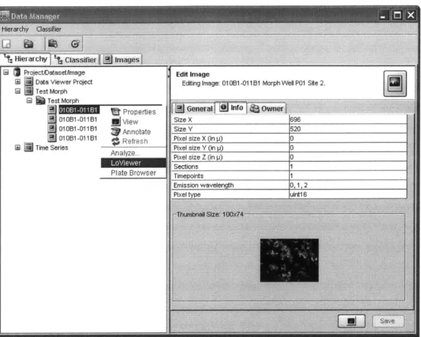
LoViewer can be used to view data for a given dataset or an individual image within that dataset. The Shoola event bus is used for launching the LoViewer. Within the current Shoola work flow, LoViewer events are created from the Shoola data manager. The data manager is a simple project viewer that presents the user with a hierarchical file manager style view of the user's projects, data sets and images. If a user clicks on a dataset or an image with the alternate mouse button, an option to load the LoViewer appears in the drop down list, illustrated in figure 1.

1:

1

f!J

W Data Viewer Project

1 Test Morph Test Morph SProperties 01 OB1I-011Bi _{l view} 01 OB1-011B1 _Annotate FI01B1-011B1 Rfreoh Time Series _Analvza

Figure 1: Shoola's data manager showing alternate click menu. The LoViewer menu item launches the Lo Viewer to visualize data for the selected image or dataset.

When LoViewer loads, a message is sent on the Shoola event bus requesting that

LoViewer load a dataset or an image. If a dataset is chosen, LoViewer will look to see

which images belong in the dataset and present the user with data points of image

granularity (meaning one data point for each image). Alternatively, if an image is

chosen, the LoViewer will look to see which features belong to the image and present the

user with data points of feature granularity. After determining which granularity of

semantic types to present to the user, the LoViewer queries the server to identify which

semantic types have stored values for all of the images in a dataset or all of the features

within an image. Once the data is loaded, the user experience in dataset mode and image

mode is identical.

The final decisions that the LoViewer makes when it is loaded are whether or not the local data store plug-in exists and whether or not there is local data for the chosen dataset or image. Through the Eclipse plug-in framework, LoViewer can easily determine if the local data store and local analysis plug-ins have been installed in the Shoola client. If the local data store plug-in has been installed, then LoViewer will present a local data tab to the user in addition to the remote server data tab. Images of these tabs can be seen in figure 2 in section 3.2.2. If the local analysis plug-in has been installed, LoViewer makes a simple call to determine if there is any local data that corresponds to the chosen dataset or image.

As has been mentioned earlier, user experience is the same once the LoViewer is initialized whether LoViewer is in dataset or image mode. For this reason, I will describe the features of the LoViewer in the following sections without making further reference to a specific mode.

3.2.2 Variable Selection

To identify meaningful relationships among semantic type values, users can plot the relationship between three variables. In the case of three variables, data points are drawn on the screen like they would be in a normal two dimensional scatter plot however the size of the data points correspond to the values of the third variable. Data points with large values are drawn larger than data points with smaller values. By providing the user with the ability to visualize the relationship between more than two variables in a single two dimensional scatter plot, many clusters can be identified that would otherwise go unnoticed.

The size of the data points is simply a qualitative cue to aid users in identifying interesting clusters of data. Because it would be difficult to map differences in quantitative values to incremental size changes of a few pixels, the values for the size dimension are scaled such that the largest value and the smallest value are assigned to

data point sizes that are aesthetically pleasing. The intermediate values are scaled in

linear fashion between the largest and smallest data point size.

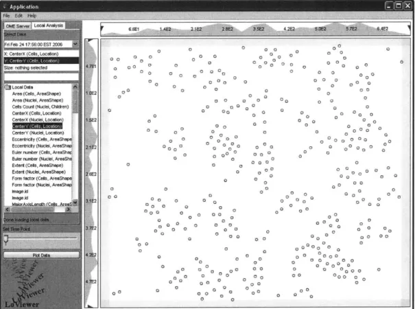
Figure 2 shows the variable selection window to the left of a data plot. To complete a

selection, users simply select a variable by clicking and then choose from the list of

available semantic types. A search field is provided for users to filter long lists of

semantic types. The search field uses a live type-ahead model whereby the selection list

is filtered as a user types, to include only the semantic types names that contain the typed

phrase. For example, if the user types ell, the filtered list would contain semantic types

with both cell and ellipse in their names.

6Z

aze: raning seectes

Qj Local Dale -Area (Cells, -AreaShape) Area (Nucel, AresShape) Cells Court (Nuclei,. Chilren) j CerterX (Cells, Location) -CarterS (Nude Localio)

CerterY (Nuclei, Location)

Eccertricilty (Cells, AreaSha Eccertriaty (Nuclei, AreaShap.

Euler number (Cals, AreaShrI Euler number (Nuclei, AreaSh% Extert (Cels, AreaShape)

Exdert (Nuclei, AreaShape) Form factor (Cats, AreaShape

Form factor (Nuclei, AreaSh* Image A Image A 0 0 0 0 00 0 0 O 0 0 0 0 0 0 0 0 0 0 0 00 0 0 0 00 00 _{0 0} 0 00 0 0 00 0 0 0 0 0 0 00 0 0 00 0 o 00 0 00 0 00 00 0 000 0 0 0 a0000 0 O0 00: 0 0 0:0 000 0 0 000 0 0 00 0 0 0 0 0 0 0 0 0 0 0 0 0 0 0 0 00 0 00 0 0 0 0 0 00 0 0 0 0 0 000 0 0 0 00000 0 00 0 00 00 0000 0 0 0 0000 0 0 00 00 0 00 0 0 0 00a0 0 0 0 00 0 00 0 0 0 0 000a00 0 0 0 0 0 0 0 0 0000 0 00 0 00 0 0 0 Oo 0 0 0 0 0 0 0 0 0 0 00 0 0 0 0 0 0 000 oo ' 00 00 0 0 00 000 000 0 0 0 0 0 0 0 0 00 00 0 00 0 000 0 0 0 00 0 0 0 00 0 000 00 0 0 0 0 0 0 0 000 0 0 o 00 Q 00 0 0 0 0 00 0 00.

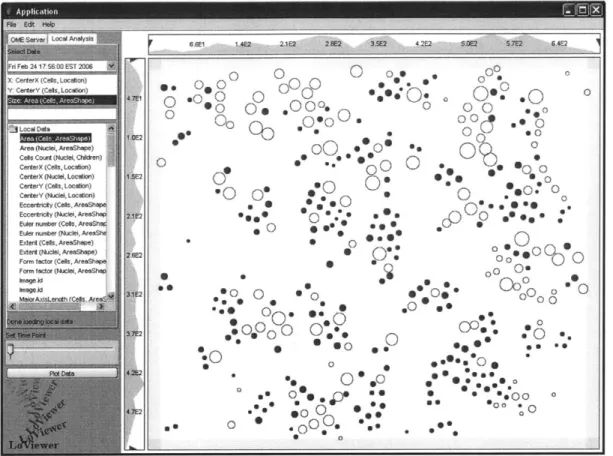
Figure 2: Example of a Lo Viewer data plot. The selection window in the local analysis tab allows the user to choose which measurements to plot. The OME server tab contains the same selection window, but points to data on the OME server as opposed to the local data store. The number bars next to the plot show the range of data values and allow the

user to define selection regions by dragging sliders.

Fr 0 0 0 0 2 0

Once the user makes a selection of at least the X and Y variables, the plot button will cause the LoViewer to plot the data for the selected values. If a third variable is selected, it will be used to determine the size of the data points. If the third variable is not selected, all of the data points will be the same size. The user is required to select both an X and Y variable because otherwise no meaningful relationship information can be determined. Initially it was thought that one variable could be presented as a histogram, but that idea was discarded in favor of X-Y plots (as will be discussed in section 3.2.4).

The internal architecture of the LoViewer supports an arbitrary number of dimensions. For example, a fourth dimension could easily be mapped to an alpha blending value for the data points. In such a case, data points with high values would appear opaque while data values with low values would appear transparent. Another dimension could be represented on a color scale. Low values could be represented in blue, high values in red and intermediate values as a suitable blend of the two colors. User feedback will ultimately determine the ideal number of dimensions required to identify unique clusters and at this time I am unable to make such assertions. As can be seen in the visual design and back-end architecture, I have left room for future development.

3.2.3 Region Selection

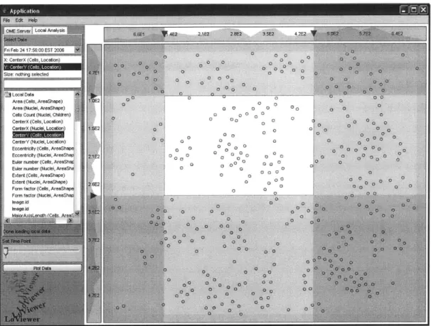
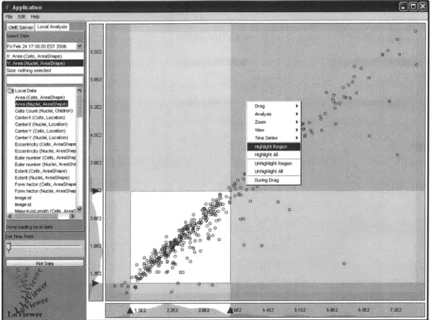
Once a plot has been made, users are able to select regions within the plot. Region selection is done by defining a beginning and an end of a region on both the X and Y axis. There are two ways to define a region initially. The first is via the range sliders that appear as triangles in the number bar displayed next to the X and Y axis. The sliders and the number bar can be seen in figure 3. As the range sliders are moved, the selected region remains visually unchanged and the unselected region is shaded out. For a faster experience, the user can define selection regions by holding the shift key and directly clicking and dragging on the plot. As the user moves the mouse, the selection window will be drawn and the range sliders moved to their appropriate positions.

Figure 3: This plot shows a selection window defined by sliders on the number bars.

Data values that are shaded out are excluded

from the selected region.

Selections can be modified in two ways as well. The first is by clicking and dragging the

range sliders. The second is by simply clicking inside of the selection area and dragging

the selection box around the plot. Clicking and dragging will move the selection region

to follow the mouse. As a selection window is dragged around the plot, the range sliders

will be updated to reflect their new positions. A selection can be quickly canceled by

holding down the shift key and hitting the alternate click button on the mouse. This

causes the range sliders to move to their statup positions at the edge of the number scales.

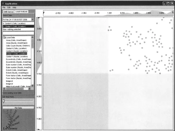
To further augment the interactive nature of the data presentation, users can pan and

zoom the display window. Panning is accomplished by holding down the space bar and

clicking and dragging in the display window. To prevent users from panning off the edge

of the plotted points, users can only pan far enough to put the corners of the data range in

the middle of the display window as can be seen in figure 4.

-2.7E2 -2.0E2 -1.3E2 -5.7E1

1

Local Data 4 Area (Cels, AreaShape)

Area (Nucei, AreaShape)

Cels Court (Nuclei, Chldren)

CerterX (Cells, Location)

CerterX (Nuclei, Location)

CerterY (Nuclei, Location)

Eccertricity (Cels, AreaShape

Eccertricity (Nuclei, AreaShap

Euder number (Cels, AreaSh* Euler numnber (Nuclei, AreaSha

E xtent (Celts, AreaShpe)

E xtent (Nuclei, AreaShape) Form factor (Cells, AreaShape Form factor (Nuclei, AreaShap

heageid hmage.id Is. 0 00 ₀ 00 0 00 0 00 0 0 0 0 0 0 00000 0 0 0 0 0 0 0 0 0 0 0 0 0 0 0 0 0 00 0 00 0 0 0 0 000 0 0 0 0 0 0 000

:

Figure 4: LoViewer prevents a user from panning off of the data range by limiting a pan such that the corner of the data range lies in the center of the screen.

Zooming is accomplished by holding down the Z key and clicking and dragging the mouse up and down. As the user pans and zooms, the values on the number bars are updated to reflect live range values. In the same way that a selection region can be canceled by hitting the alternate click button while holding down the shift key, zooming can be canceled by hitting the alternate click button while holding down the Z key. If a zoom is canceled, the LoViewer will return to its default zoom level which is a zoom-to-fit setting at which all data values are shown in the display window.

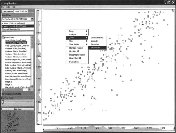
In addition to interactive pan and zoom operations, users can let the LoViewer determine optimal viewing conditions. By using the alternate mouse button to click on the display

window, the user can select from a list of several zoom operations. The user can choose

a default zoom-to-fit level or a zoom level that displays only the chosen selection region.

Additionally, the user can increase or decrease the zoom level by a given percentage.

This alternate click menu can be seen in figure 5.

Obll: erverj LoahfAnelysls

FriFeb 24 17,56:00 EST 2006 2.E

KCAealr (Cels, LreSo)

Stze. nothing selected

26E2 ,tjLocal Date

Area (Cells, AreaShape) ;

Cal Coun (Nuclei, Chldlren)

CenterX (Nuclei, Locaton) CerterY (Cols, Location) CerterY (Nuclei, Locaton) Eccertncity (Cells. AreaShap Eccertrly (Nuciei, AreaSha

Euler number (Cls, AreaShal

Euer number (Nuclei, AreaShe Extert (Cels, AreaShape)

Extert (Nuclei, AreaShape) Form factor (Cells, AreaShap Form factor (Nuclei, AreaShap

kmaged

Drag

Analysis b0 0

Zoom Selected 0 000

New I ZoomI 0 0 0 0

Time Series I Zoom Out "0 o 0 0

W g i Rgte g o n 0 0 (9 -l ight AN 0 Unhrhgt Region 0 0 0,.. 0 During Drag 0 0 OS at 0 0 0 0 00 0 0? 0

~d

Figure 5: LoViewer alternate click menu showing options that the user can select to change the zoom level.

3.2.4 Single Axis Histograms

Initial plans for LoViewer included histograms. I had thought the histograms would be a

valuable tool for identifying the distribution of certain variables and would be generated

when a user selected only one variable to display. However, using the main display

window for a histogram seemed a waste. It was decided to always show a histogram in

the background of both the X and Y number bars under all display conditions, regardless

~0

0

0

of zoom level and panning position.

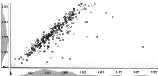
The single axis histograms are generated on the fly and they provide a powerful visual cue to help the user identify the general trend of X and Y variables individually. As the user pans and zooms to different regions of data, the histograms are updated to reflect a local distributions of the data point values in the current viewing window. These histograms can be seen in figures 6 and 7.

3.2E2 ( 20 _%0 -@ 0 0 0 0 0 0 o 00 0E 0 1,9E2 0 0

Figure 6: Histogram shown in the number bars

for

0 00 0 0 0 0 b00 0 8 0 a, o? 0 0 0 0D 0 CP 9 o n b 0 0 0 0 0 08 0 ro 0 0 00 n0 0 igb a po t2 i 4

By showing histograms at all times, the efficiency of the LoViewer data scrubbing experience is greatly increased. For example, range sliders can quickly be set to values that correspond to meaningful points in the histogram plots of a variable's distribution. Additionally, users can instantly identify if a measurement is distributed according to a commonly recognized distribution such as a uniform or normal distribution.

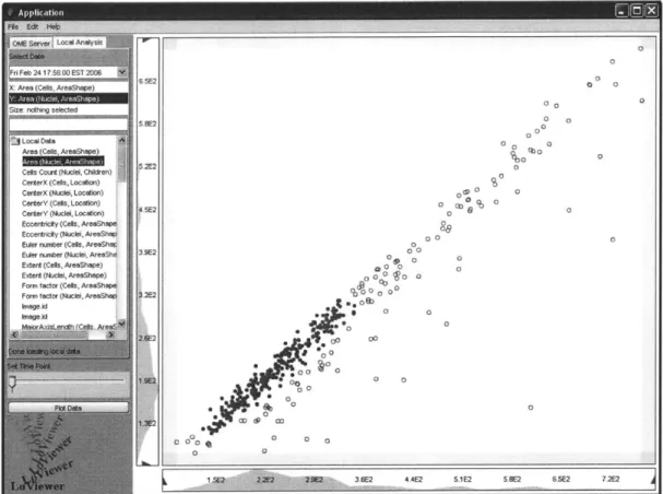
3.2.5 Data Point Selection

Selection regions can be used to select and highlight data points directly. After a selection region is set, the user can use the alternate mouse button to click anywhere in the display window and get a menu allowing the data points within the selection region to be selected or deselected. Another method of selecting data points is a highlight while

dragging option in the alternate click menu. This option causes the data points inside a

selected region to be selected and the points outside of the selection region to be deselected interactively as the selection window is modified via any method described in section 3.2.3. The alternate click menu for selecting data points can be seen in figure 8.

Figure 8: LoViewer alternate click menu showing options that the user can select to highlight data points.

Data point selections are internally mapped to the unique OME identification values that

correspond to the images or features that each data point is associated with. This

association is important because it means that once a set of data points is selected, the

selection is maintained across different plots. This idea can be seen in figures 9 and 10.

X: Area (Cells, AreaShape) Size: nothirg selected

$|Local Date

Area (Cells, AreaShape) Cels Count (Nuclei, Children)

CenterX (Cells, Location) CenterX (Nuclei, Localon) CenterY (Cels, Location) CenterY (Nuclei, Loceim)

Eccentricity (Cels, AreaShWp. Eccentricty (Nuclei, AreaSh*

Euler number (Cels, AreaSha

Euler number (Nuclei, AreeShd Extent (Cels, AreaShape)

Extent (Nuclei, AreaShape) Form factor (Cells, AreaShwp' Form factor (Nuclei, AreaShap

Inageid Imageild 6.5E2 5.8E2 58E2 3 2E2 2 E2 0o 0 0 0 0 0 0 0 00 00 00 0 .ago . . oC 0 6000 0 0 0 0 0 a 00 0 0

4.4E2 5.1E2 S.E2 65E2 7.2E2

Figure 9: Data points are selected in a region of interest based on the between two plotted variables.

relationship ~,~Cd7l7%izl55izl, 3.6E2 k 1 5E2 2-2C2 2 OE!2 0 0 0 0

Ol01 AO8YSI 4E2ot L2C 3 Sf2 4ie ?E 5 D1 Siw2

X: CeerX (Ce0s Locaon) 0 . 0 0

Y: CenterY (Cells, Locaton) - 4 _0. 0 0O OEJ _{0 0 00} 60C _{00 0 .*} **4.' 0 0* a ₀ 00o0

S-o.0 0 .. 0 ) C u .00

- -- 00 0 .

Ae(Nce.eShape -o _*O.

Cels Count (Nuclei, Chiren) 0 0 a 0 0 2)

CenerX<Cas.Locaon) It 1 0 * o o 0

CerterX (Nuclet, Location) 11E2

. 0

CerterY (Cels, Location) 6 . .* O _{.* 0}

CerterY (Nuclei, Location) 00 _{O0 0}

Eccentrcity (Cels, AreShp g

Q

Eccentriciy (Nuce, k.eaShap 0 : a a ) .* .. .

Euler nurmber (Cels, AresShGK 0 go a * -P . 1P*

Euler number (Nuclei, AeaShe0 0

E xt (Ceas, ArShape)0 so

Extent (Nuclei, AreaShape) E ₀

Form factor (Cels, AreaShape 0 0

Form factor (Nuclei, AreaShap oa

C 0 0 .

Qc.

ta n e.lls CrA- C , Arm- *4 * *0

.0. oO

0

0*.O

~

Figure 10: A previously defined selection is maintained when the data points are plotted against different variables. Here we can see that the data points that were previously selected are evenly distributed across the image based on their X and Y position and that

they do not correspond to the large cells in the image.

Data point selection is a significant step in the data scrubbing process. Once users are

able to identify data points that belong to interesting clusters, the final step in the

high-content analysis process is to examine the images or features that the data points

correspond to. This idea will be discussed in the next section.

3.3 Shoola Integration

As has been mentioned earlier, the Shoola framework allows individual plug-ins to

communicate with each other via the Shoola event bus. The data point selections

described in the previous section give LoViewer the ability to direct careful analysis on

subsets of high content biological screens. The Shoola event bus allows LoViewer to fire off messages to other tools requesting further analysis of interesting data.

Depending on project goals, it might be important for a researcher to view a collection of images that correspond to interesting data points. Additionally, it might be important for a researcher to view a single high resolution image and overlay regions of interest that correspond to selected data points. In a much simpler case, researchers might just want to record a classification of the data points to allow them to be revisited in the future.

Tools to conduct these additional analytic steps are currently being developed by other OME development sites. Unfortunately, because the OME project is currently migrating from the OME server to the OMERO server, the Shoola client is in a state of flux and final versions of these tools are not yet available. As a result, the LoViewer currently does not interface with a classification tool or a region of interest tool, but implementing such interfaces will be straightforward once the necessary Shoola tools are finalized.

4 Design and Implementation

The LoViewer exists as a plug-in for Shoola, the OME Java client. Because the Shoola client was recently redesigned to incorporate Eclipse-style plug-in bundles, component development has become extremely simple. To connect the LoViewer application to the Shoola client, several minor configuration files need to be created and a plug-in needs to be exported through Eclipse IDE. There are ways to develop plug-ins outside of the Eclipse IDE, but using the IDE makes plug-in development extremely simple. Without having to weave the LoViewer into a complicated tangle of interdependent code, I was able to focus on developing a stand alone plug-in that brings unique functionality to the Shoola client. The layout of the LoViewer's components can be seen in figure 11.

-cn b s a 0 I I

4.1 LoViewer Overview

LoViewer can run in both image and dataset mode on both local and remote data, but its overall functionality is consistent. Data values are used to generate scatter plots in an attempt to allow researchers to identify relationships that produce interesting clusters. In the first mode, LoViewer displays data belonging to an entire dataset. In this dataset mode, each data point corresponds to a single image within the dataset. In a second mode, LoViewer displays data belonging to a single image. In this image mode, each data point corresponds to a single feature within the image. The third and forth modes exist as variations to the dataset and image browsing mode. The third mode for LoViewer consists of browsing local data across an entire dataset. The fourth mode consists of browsing local data within a single image.

Because the local data store is extremely fast, the LoViewer also has a fifth and sixth mode that correspond to viewing local data over time in either dataset or image mode. If an analysis is run on a time series image, the local data store is able to rapidly return data values to the LoViewer with a small enough latency that the user can smoothly move a slider to view data points belonging to different slices in the time series. This mode is only available for local data because there is too much latency between the Shoola client and an OME server in its current implementation.

4.2 LoViewer as part of Shoola

As a component of Shoola, the LoViewer is able to take advantage of the abstraction layer provided by Shoola between the OME database and pure Java objects. Additionally, the LoViewer is able to communicate with other Shoola components to provide new functionality and extend the capabilities of existing Shoola tools.

4.2.1 LoViewer Agent within Shoola

Through the use of the plug-in structure of Shoola, LoViewer establishes itself as a Shoola agent. All of the individual components in the Shoola client exist as agents. Agents communicate with each other through the Shoola event bus. When an agent is initialized, it registers itself with the event bus and specifies what classes of event messages it wants to listen for. Once the agent registers itself on the event bus, it is able to receive messages that are posted to the event bus by other Shoola agents. Furthermore, agents are able to post messages to the event bus in order to pass messages to and drive actions in other agents.

4.2.2 Message Handling

When LoViewer is initialized, it registers with the event bus to listen for LoViewerPluginEvent messages. If an agent posts a LoViewerPluginEvent message to the event bus, LoViewer is launched and the parameters of the data browsing

message as well as a handle to the Shoola registry are passed into the LoViewer initialization class. LoViewer then checks to see if it has received a request to view a dataset or an image. At initialization time, LoViewer enters either dataset or image mode. This decision is held in the LoViewer's manager class and it is referenced at various points by internal classes to determine how to access the semantic types that are associated with either images or features.

4.2.3 Loading a Dataset/Image and Image/Feature data

In dataset mode, the LoViewer receives a message from the Shoola bus that contains a Dataset object. LoViewer must then extract the dataset ID and make calls to the Shoola API to request a list of images that belong to the dataset. In image mode, LoViewer receives a message from the Shoola bus that contains an Image object. LoViewer must then extract the image ID and make calls to the Shoola API to request a