Do Environmental Policies Hurt Trade Performance?

HAL Id: halshs-00939249

https://halshs.archives-ouvertes.fr/halshs-00939249

Preprint submitted on 30 Jan 2014

HAL is a multi-disciplinary open access archive for the deposit and dissemination of sci-entific research documents, whether they are pub-lished or not. The documents may come from teaching and research institutions in France or abroad, or from public or private research centers.

L’archive ouverte pluridisciplinaire HAL, est destinée au dépôt et à la diffusion de documents scientifiques de niveau recherche, publiés ou non, émanant des établissements d’enseignement et de recherche français ou étrangers, des laboratoires publics ou privés.

Jean-Louis Combes, Pascale Combes Motel, Somlanaré Romuald Kinda

To cite this version:

Jean-Louis Combes, Pascale Combes Motel, Somlanaré Romuald Kinda. Do Environmental Policies Hurt Trade Performance?. 2014. �halshs-00939249�

C E N T R E D'E T U D E S E T D E R E C H E R C H E S S U R L E D E V E L O P P E M E N T I N T E R N A T I O N A L

SERIE ETUDES ET DOCUMENTS DU CERDI

Do Environmental Policies Hurt Trade Performance?

Etudes et Documents _{n° 04}

January 2014

CERDI

65 BD. F. MITTERRAND

63000 CLERMONT FERRAND - FRANCE TÉL. 0473177400

FAX 0473177428

The authors

Jean-Louis Combes

Université d’Auvergne, Centre d’Etudes et de Recherches sur le Développement International (CERDI), CNRS, UMR 6587, F-63009 Clermont Fd, France.

Email: j-louis.combes@udamail.fr

Pascale Combes Motel

Université d’Auvergne, Centre d’Etudes et de Recherches sur le Développement International (CERDI), CNRS, UMR 6587, F-63009 Clermont Fd, France.

pascale.motel_combes@udamail.fr

Somlanare Romuald Kinda

Université d’Auvergne, Centre d’Etudes et de Recherches sur le Développement International (CERDI), CNRS, UMR 6587, F-63009 Clermont Fd, France.

Email: somlanare.kinda@udamail.fr - Corresponding author

La série des Etudes et Documents du CERDI est consultable sur le site :

http://www.cerdi.org/ed

Directeur de la publication : Vianney Dequiedt Directeur de la rédaction : Catherine Araujo Bonjean Responsable d’édition : Annie Cohade

ISSN : 2114 - 7957

Avertissement :

Les commentaires et analyses développés n’engagent que leurs auteurs qui restent seuls responsables des erreurs et insuffisances.

Abstract

This paper contributes to the controversial literature on the relationship between environmental policies and international trade. It provides new evidence about the effect of a gap in environmental policies between trading partners on trade flow on a sample of developed and developing countries over the 1980-2010 period. The paper innovates on two aspects. First, while previous studies have used partial measures of environmental regulations (input-oriented or output-oriented indicators), an index of a country’s environmental policy is computed. This index is calculated as the difference between observed pollution levels and “structural” pollution i.e. pollution predicted by determinants of environmental degradation as identified and modelled in the literature. This index is therefore a measure of “revealed” efforts made by countries aiming at downsizing environmental degradation. Second, the effect of these revealed environmental policies is assessed on bilateral trade flows in a gravity model. A particular attention is paid to similarities in environmental policies. Our results show that a gap in domestic efforts towards environmental protection between trading partners has no effect on exports. Moreover, the results do not appear to be conditional on the level of development of the countries trading nor on the characteristics of exported goods (manufactured goods and primary commodities).

Keywords:

Trade, Environmental policies, Gravity model

JEL Classification: F14, F18, Q56

1

1

Introduction

In the 1990s, the debate around NAFTA revived the debate on trade and the environment (Grossman & Krueger 1991). Antweiler et al. (2001) addressed theoretically the question of whether freer trade hurts the environment, and concluded that it did not. This result was in the spirit of the Doha Round launched in 2001, which objectives comprise specific discussions on trade and the environment. This incantatory affirmation of win-win outcomes for trade, the environment and sustainable development, which has turned into the “Doha blues” (Jones 2010; Abbas 2011), is at odds with the prevailing idea of increasing ecological scarcities and environmental degradation (Barbier 2011; Rockström et al. 2009). Indeed, knowledge and the analysis of global environmental threats improved substantially and has steadily fuelled concerns about environmental degradation. For instance, the Stern Review on the Economics of Climate Change (Stern 2007) highlighted the effects of climate change on global welfare, economic growth prospects and development. Climate change certainly entails a differentiated effect on developing countries (Mendelsohn et al. 2006). It may threaten the ability of developing countries to target the Millennium Development Goals set for 2015.

Countries have been encouraged to implement environmental policies particularly since the 1972 meeting of the United Nations Conference on the Human Environment in Stockholm. Since then, environmental policies have been enforced in many developed countries. The US Environmental Protection Agency was created in 1970 and accompanied the “command and control era” during which several amendments were introduced to US environmental regulation (Portney 2007). In the same decade, the first EU Environmental Action Plan was decided, in 1973, and initiated the EU environmental policies which had tended to integrate within more global strategies such as the World Conservation Strategy advocated by the IUCN. Countries have committed themselves to international environmental agreements. In the wake of the Rio conference in 1992, a new generation of those agreements came into force and the Kyoto Protocol is the first example of a binding commitment to an environmental issue even though its scope

2 appeared to be limited. The debate about the effect of environmental policies, either domestically rooted or induced by international law on trade and growth, is still lively.

Hallegatte et al. (2012) argue that environmental policies may contribute to economic growth and sustainable development. First, environmental policies that sustain and enhance natural capital assets (fisheries, soils and forests) on which populations rely on for their livelihoods, have the potential to create jobs and therefore increase incomes. For instance green investments may potentially increase employment in the energy sector i.e. wind energy, photovoltaic and biofuels sectors (Zenghelis 2011). Secondly, environmental policies may generate externalities. Economic activities in the tourism sector, which hinges upon natural assets, may increase population income and allow them to increase their resilience. Better air and water quality are crucial for population health and thus labour productivity. Thirdly, environmental policies can change the production frontier through innovation development and dissemination. Several authors believe that strong environmental policies can stimulate competition and exports through innovations (Porter 1991). This is the so-called Porter hypothesis which has been the subject of several theoretical developments within the endogenous growth framework (Acemoglu et al. 2012).

On the other hand, it may be argued that environmental policies entail not only transaction costs (McCann et al. 2005) but potentially impede competitiveness. This is a consequence of the pollution haven hypothesis, according to which a firm’s localisation decisions are partly based on weak or poorly enforced environmental rules. Non-stringent environmental policies and a race to the bottom supposedly create comparative advantages. Empirical evidence of the pollution haven hypothesis is mixed (Grether & Melo 2003) although recent results do not invalidate it (Kellenberg 2009; Levinson & Taylor 2008; Millimet & Roy 2011).

This paper is an attempt to add to the literature on the effect of environmental policies on trade. The contribution is two-fold. First, we focus on the measurement of environmental policies which are usually labelled as either input-oriented or output-oriented indicators. The former derive, for instance, from public research and development expenditure, investment expenditure in pollution abatement technologies, “green” taxes, or multilateral environmental agreements. The latter more simply

3 measure environmental outputs such as emission intensities, emissions per capita, or soil or water quality. Input oriented indicators are not always available for all countries however, and output oriented indicators may not solely depend on policies with environmental purposes. We therefore propose here to consider a modified output oriented index that is an index of revealed environmental policies of which methodology is developed in other papers. It allows an estimation of domestic efforts (Combes & Saadi-Sedik 2006; Combes Motel et al. 2009; Boussichas & Goujon 2010; Guillaumont & Guillaumont 1988) in a manner reminiscent of the Chenery and Syrquin approach to identifying structural change (Chenery & Syrquin 1975). Second, contrary to most previous studies that analyse the effect of domestic environmental policies on trade (total or bilateral), the effect of a similarity in environmental policies on trade flows between partner countries is highlighted. Indeed, countries either rely on different environmental policy instruments or are engaged in different international agreements. This may result in different policies and results.

The rest of the paper is organized as follows. Section 2 provides a literature review of the theoretical effects of environmental policies on bilateral trade. Section 3 presents the methodology to compute domestic efforts for environmental protection. Section 4 evaluates how far environmental policies have an effect on bilateral trade flows using a gravity model over a sample of developing and developed countries on the 1980 2010 period. Section 5 presents results and the last section is devoted to concluding remarks and implications.

2

Relationship between environmental policies and trade

This section reviews the way environmental policies may hamper or spur trade flows.

2.1 Environmental policies and trade costs

Several authors (Kellenberg 2009; Levinson & Taylor 2008; Millimet & Roy 2011) believe that the implementation of environmental policies may reduce the competitiveness of economies. Environmental policies can take several forms, such as command and control or market-based instruments, and can generate additional costs and burdens on domestic firms. If these costs are high, they may hurt the competitiveness of domestic firms compared to foreign ones operating under weaker

4 environmental policies. Polluting firms may relocate from countries with stringent environmental regulation towards countries with weaker rules. This is known as the pollution haven hypothesis: weak environmental regulations are a source of comparative advantages and modify trade patterns towards dirty goods (Liddle 2001). Moreover, since environmental quality is a normal good, demand for environmental regulations may be higher in developed countries than in developing countries.

Theoretical models and studies suggest a negative link between environmental regulation costs and trade flows. Using a theoretical model where the manufacturing sector differs in primary factors (labour, capital) and pollution intensity, Levinson & M. S. Taylor (2008) show a positive relationship between pollution abatement costs and a country’s imports. Peters et al. (2011) provide evidence of carbon leakage. They show that the implementation of environmental policies and agreements in developed countries has increased the imports of polluting intensive goods from developing countries. In addition to compliance costs (for example expenditures on control and new equipment monitoring), Ryan (2012) shows that environmental regulations increase costs and market power. For instance, sunk costs of entry of firms into U.S. markets have significantly increased under the Clean Air Act (CCA). Consequently incumbent firms have benefited from increased market power.

Few studies (Van Beers & Van Den Bergh 1997; Cagatay & Mihci 2006; Keller & Levinson 2002) found a negative effect of environmental regulation on trade patterns. Van Beers & Van Den Bergh (1997) highlight that a divergence between the environmental regulations of developing and developed countries negatively impacts pollution-intensive goods trade (mining, non-ferrous metals, or chemical products). Cagatay & Mihci (2006) found that they had a negative effect on pollution intensive goods. Using the propensity score matching method, Aichele and Felbermayr (2013) analyse the effect of Kyoto Protocol commitments on bilateral exports. They show that Kyoto commitment has cut the exports of Kyoto countries by 13 - 14%. Energy intensive industries such as iron and steel, non-ferrous metals, and organic and inorganic chemicals, are highly affected.

Moreover, according to Dean et al (2009), the attractiveness of environmental regulations to foreign investments in China is conditional on the investor´s source

5 country and the industry characteristics. The study concludes that investment from high income countries and non-polluting industries are not attracted by weak environmental regulations.

Tobey (1990) and Cole & Elliott (2003) do not evidence of any relationship between environmental regulations and pollution intensive industries, nor net exports. Trade flows are explained instead by differences in factor endowments (capital, labour, natural resources). A similar result was found by Xu (2000). The lack of evidence in support of the negative effect of environmental regulations on trade may be explained with two reasons. For most industries, environmental costs are smaller than other costs and consequently the effect of environmental policies on international competitiveness are probably minor (Nordström and Vaughan (1999). Further, gains from trade are generally sufficient to pay for additional abatement expenditures and other regulatory costs. Jug & Mirza (2005) consider that the effect of environmental regulations is related to the degree of product differentiation. They show that environmental stringency has less effect on the trade of differentiated goods with a low price elasticity. Albrecht (1998) explains the non-negative impact of environmental regulations through the fact that many developed countries have diversified exports and that most studies do not focus on specific products.

2.2 Environmental policies and innovation

Environmental policies may also have a positive effect on trade flows. Porter (1991) and Porter & Van der Linde (1995) explain that tougher environmental policies stimulate technological innovation, thereby increasing productivity and competitiveness. They dismiss the pollution haven hypothesis as a supposedly static perspective which therefore does not take in account the reactions and behaviours of firms confronted by environmental regulations. When firms face potentially high abatement costs, they will be incited to change production routines, invest in innovative activities and find new ways to achieve environmental objectives and product new marketable goods. They may become more aware of new methods of production that reduce production costs (through increased efficiency, decreased resource inputs) and increase the quality and competitiveness of products. This is the so-called Porter hypothesis, according to which environmental policies may stimulate innovation opportunities, and improve the productivity and competitiveness of countries.

6 Three arguments may support the Porter hypothesis. The first one is the strategic effect inside firms. Sinclair-Desgagne & Gabel (1997) assume that firms have myopic behaviours. The implementation of environmental policy can incite them to reconsider existing routines and improve business performance. Xepapadeas & de Zeeuw (1999) for instance, found that environmental regulations such as emission taxes increase a firm’s productivity and profits.

The second argument relies on strategic effects between firms. Mohr (2002) developed a theoretical model in which productivity gains are associated with learning by doing. In other words, the productivity of a new green technology is a function of the total accumulated experience in the industry. Because no firm is forced to bear the burden of adopting green technologies (the initial learning costs), governments may promote them with stringent environmental policies. By imposing environmental policies, the government may incite domestic industries to invest in research and development activities (Simpson & Bradford 1996; Greaker 2003). They can acquire strategic advantages and improve their competitiveness in international markets through better access to markets, the possibility of differentiating products or selling pollution-control technology (Lanoie et al. 2011). Using survey data from 78 European firms operating in the building and construction sector, Testa et al. (2011) showed that environmental policies (measured by inspection frequency) have a positive effect on investments in advanced technological equipment, innovative products and business performance. Albrecht (1998) evidences that countries with relatively active environmental regulatory (national ozone policy) have improved their competitiveness of CFC- using manufacturers. Similarly Costantini & Mazzanti (2012) show that, for the EU15 over the period 1996–2007, the high technology sector was positively affected by energy and environmental taxation whereas the more energy intensive medium and low technology sectors were not affected. Some authors (De Santis 2012; Trotignon 2011) believe that the positive effect of environmental regulations on trade flows may be related to multilateral environmental agreements (MEAs) or regional trade agreements which allow trade creation and the diffusion of environmental-related production standards.

The third argument is that the implementation of environmental policies may contribute to increasing environmental awareness and affect the preferences of

7 consumers. Firms are forced to produce new goods in order to survive. Realising a literature review on theoretical foundations and empirical studies on the Porter Hypothesis, Ambec et al. (2013) show that several recent studies support it. These recent results are explained by a heightened social awareness and responsibility for sustainable development. In a world characterised by improving environmental performances, firms and industries are more able to become competitive and produce green goods.1

3

How to measure environmental policy?

We review here existing indicators and propose our methodology for the implementation of revealed environmental policies.

3.1 Existing indicators of environmental policies

Input-oriented indicators are input efforts devoted to environmental protection. Several authors use public research and development expenditures, current investment expenditures in pollution abatement and control, energy tax, or the number of multilateral environmental agreements signed by countries, as proxies for environmental policies. However there are two limits to this approach: the enforcement of multilateral agreements and the lack of data on wide time and geographical coverage for some inputs.

Van Beers & Van Den Bergh (1997) believe that output oriented indicators are better proxies for environmental policies. Indicators used in the economic literature include emissions intensities (SOx, NOx, CO2, and SO2), emissions per capita, or other pollutants related to water or soil quality. The main limitation of these indicators is that output oriented indicators may depend on environmental policies as well as on structural factors. For instance, several determinants of pollution may be out of a government’s hands. These are related to long term economic development, business cycles, demographic dynamics or international prices.

1 _{This effect is somehow in the same vein as the “pollution halo” hypothesis according to which better} technologies and management, green preferences of consumers in developed countries raise environment friendly technology transfers and know-how. See Zarsky (1999) for a review.

8 We thus want to disentangle those structural factors from policies and measures dedicated to achieving better environmental quality. From our point of view, comparing observed to “structural” environmental degradation may deliver a proper measure of environmental policies.

3.2 An indicator of revealed environmental policies

This approach has been used by other authors. Combes & Saadi-Sedik (2006) built an indicator of a trade policy’s openness or revealed trade policy whereas Combes Motel et al. (2009) estimate an indicator of policies against deforestation. Structural environmental degradation is obtained by calculating the level of pollution a country should have as a result of its structural characteristics. The indicator of revealed environmental policy is the difference between observed pollution levels and structural pollution. It captures revealed environmental policies, based on their results. The main interest in this approach is that it provides a standardised measure of the environmental efforts of countries; it also avoids subjectivity in the choice and weighting in the combination of several environmental policy instruments. Another interest is that the measure of structural environmental degradation may be based on economic theory explaining environmental degradation.

More formally, let us assume that environmental degradation _, of country i at period t depend on a vector _, of structural factors:

, = , + , (2)

The error term _, provides the measure of revealed environmental policies:

, = , − , (3)

Environmental policies are said to be efficient when the observed environmental degradation is lower that the predicted structural level i.e. when _, is significantly negative. This indicates that environmental policies are successful in the mitigation of environmental degradation. On the other hand, environmental policies fail when _, is significantly positive. This may be the outcome of policy as well as market failures. It is worth noting that since _, is the error term; its average value is zero: this indicator is relative.

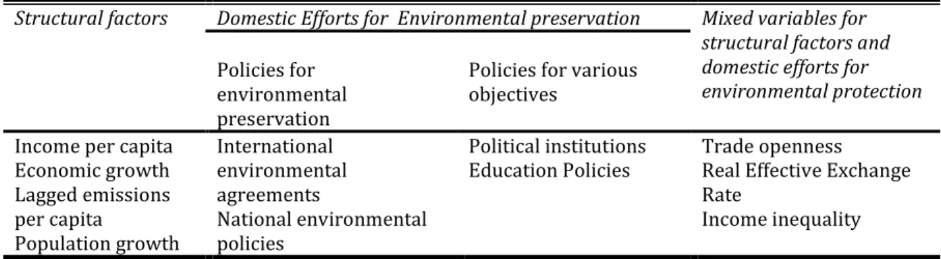
9 3.2.1 How to identify structural and mixed determinants of environmental degradation A measure of revealed environmental policies requires identification of the structural factors of environmental degradation. Table 1 classifies those structural factors: income per capita, population growth, economic growth and lagged level of emissions. Other factors of environmental degradation may be related to specific policies. These policies are of two sorts. First, environmental mitigation can be the result of domestic initiatives. For instance, environmental commitments, as defined by international environmental agreements, contribute to domestic environmental efforts. Secondly, environmental degradation is also influenced by other policies such as education policies, industrial policies or policies targeting more efficient institutions. The classification of other factors between structural determinants, domestic efforts of environmental protection and other policies may be questionable. These factors are trade openness, the real effective exchange rate (REER) and income inequality. Table 1 below summarises our characterisation of the determinants of environmental degradation.

Table 1: Classification of main variables related to environmental degradation

Structural factors Domestic Efforts for Environmental preservation Mixed variables for structural factors and domestic efforts for environmental protection

Policies for environmental preservation

Policies for various objectives

Income per capita Economic growth Lagged emissions per capita Population growth International environmental agreements National environmental policies Political institutions

Education Policies Trade openness Real Effective Exchange Rate

Income inequality

3.2.1.1 Income per capita

The relationship between income per capita and environmental quality has been widely studied in literature. According to several authors, environmental quality first deteriorates and then improves as income per capita increases (Grossman & Krueger 1995; Antweiler, Copeland, & Taylor 2001). In other words, environmental quality may be considered a luxury good in the first stage of development. Poor people are more concerned with food and other essential needs and less concerned with environmental protection. At higher income levels, people want higher levels of environmental quality. Moreover, higher incomes enable higher public expenditure on environmental infrastructures, as well as environmental policies that drive private sector expenditure

10 towards abatement technologies. Income per capital is a structural factor of environmental quality: it is often considered in the literature as an “underlying” factor that characterises overall economic conditions. Moreover, a nonlinear effect of income per capita can also be tested in accordance with the Environmental Kuznets Curve.

3.2.1.2 Economic growth

It is assumed that the economic climate or economic growth may have an ambiguous effect on environmental degradation for two reasons: a positive effect may be explained by structural change in the economy, from the industrialised sectors to the manufacturing and service sectors. A negative effect on environmental quality may be explained by a change of economic structure from agricultural to industrialised sectors. Moreover, when economic growth slows, countries are not incited to implement environmental policies.

3.2.1.3 Population growth

It is generally assumed that population pressure is a driver of environmental degradation. This idea is popularised by the well-known IPAT identity (Ehrlich & Holdren 1971). Access to food or to energy involves, for instance, emissions of greenhouse gases. Holdren (1991) shows the contribution of population growth to greenhouse gas emissions as being responsible for 40% (36%) of the increase in energy consumption (annual emissions growth) respectively. Shi (2003) finds that the effect of population growth on pollution is higher in developing countries than in developed countries.

3.2.1.4 Lagged level of emissions per capita

This variable may be a determinant of current levels of air pollution. The latter may be justified by inertia in environmental degradation. It may be also the result of convergence in environmental degradation, i.e. emissions, as theoretically established by Brock & Taylor (2010) and tested by Kinda (2010). Lagged emissions, as justified by the convergence hypothesis, belong to the set of structural determinants of current environmental degradation.

11 3.2.1.5 Trade openness

Grossman & Krueger (1995) decompose the effects of trade on environmental quality into scale, technical and composition effects. The scale effect of trade measures the negative environmental consequences of scalar increases in economic activity. The technical effect is the positive environmental consequence of increases in income, which call for cleaner production methods. The composition effect can have a positive or negative impact on the environment because it measures the evolution of the economy towards a more or less appropriate productive structure. Thus, Antweiler et al. (2001) conclude that trade reduced the pollution emissions of 43 countries over the period 1971-1996. According to Frankel & Rose (2005), trade is favourable to the reduction of pollution. However, other authors such as Magnani (2000) highlights a negative impact of trade on carbon dioxide emissions.

Discussing the effect of trade openness on the environment illustrates how difficult it is to establish a clear-cut delimitation between structural determinants and domestic policies. Indeed Combes Motel et al. (2009) and Combes & Guillaumont (2002) disentangle the natural openness that is explained by structural factors (size of countries, geographical characteristics) from outward-looking policies implemented by governments which have cut tariffs or withdrawn restrictions or quotas. In Table 1, policies favouring trade openness are considered as a mixed variable: they may partly channel the influence of structural factors on environmental degradation.

3.2.1.6 Income inequality

The effect of income inequality on environmental quality has been analysed by many scholars. Magnani (2000) and Koop & Tole (2001) found that inequality of income tends to exacerbate pollution and deforestation respectively. Political economy models provide theoretical arguments according to which income inequality increases environment degradation through the rate of time preference (Boyce 1994). Indeed, income inequality reduces awareness of environmental quality for both rich and poor: the poor would overexploit natural and environmental resources to ensure survival. Moreover, income inequality and a polarization of resources increase and exacerbate conflicts (violence, social troubles). Rich people seem to prefer a policy of overexploiting the environment and natural resources and investing the returns abroad. Torras &

12 Boyce (1998) assume that political power is highly correlated with income inequality: in unequal societies, those who benefit from environmental degradation (the rich) are more powerful than those who bear the costs (the poor). Therefore, the cost-benefit analysis predicts environmental degradation as a result of income inequality. Borghesi (2006) argues that the implementation of environmental policies is more likely with social consensus. It is easier to get this consensus in an equal society that in an unequal society with conflicts between political agents and social instability.

However other scholars believe that income inequality may have no effect or improved environmental quality. Ravallion et al. (2000) claim that the impact of income inequality on environmental degradation depends on the marginal propensity to emit (MPE). If the poor have a higher (lower) MPE than the rich, a reduction of income inequality will increase (reduce) pollution emissions respectively. One cannot predict a

priori which of these two effects will happen. Indeed, the poor may consume goods with

more (or less) pollution than the rich. Therefore the effect of income inequality is not clear and depends on whether the MPE increases or decreases as income grows. In other words it depends on the second derivative of the pollution-income function.

Similarly to trade openness, we may suppose that inequality of income may be explained simultaneously by structural factors and by policies (social and economic). Indeed, Milanovic (2010) shows that income inequality is determined by income per capita, the ideology (religion), and the quality of democratic institutions that favour redistribution policies.

3.2.1.7 Real effective exchange rate (REER)

The real effective exchange rate may affect environmental degradation. Arcand et al. (2008) show that real exchange rate depreciation may reduce environmental protection in developing countries, and has the opposite effect in developed countries. The REER depends on international prices, which are structural factors, but also on economic policies. The REER is therefore a mixed variable according to the typology of Table 1.

13 3.2.2 How to measure domestic efforts towards environmental protection?

3.2.2.1 Econometric model and results

The measurement of domestic efforts towards environmental protection is made on a panel of 128 countries over 1980 to 2010. Data are compiled in five-year averages. The panel data regression takes the following form:

, = + , + + , (4)

, is the measure of environmental degradation. Two indicators2 are used: carbon

dioxide per capita (CO2) emissions and sulphur dioxide per capita (SO2). Country fixed effects are taken into account and control for time invariant structural determinants. Period fixed effects allow controlling for omitted variables that are common to the countries (e.g. international prices). As explained in section 3.2, the residual of this regression is labelled domestic effort for environmental protection (DEEP).

Equation (4) may be estimated with different econometric methods (ordinary least squared (OLS), fixed effects (FE), and random effects (RE)). However these methods are inadequate because the former (OLS) does not take unobserved heterogeneity of countries into account and the latter (FE, RE) are inadequate for dynamic models. Because our model is a dynamic panel, we use the GMM-System (Generalized Method of Moment) from Arellano & Bond (1991), Arellano & Bover (1995) and Blundell & Bond (1998).

The GMM-System (Generalized Method of Moment) is a method that estimates a system of two equations: one equation in level and the other in first differences. In the first estimate, we use lagged variables in levels of at least one period as instruments of the equation in first differences. It removes unobserved time invariant and unobserved individual characteristics. The conditions to be met are that the error terms are

2 _{In the absence of a single measure of environmental quality, many indicators have been used in the} literature as a proxy for environmental quality. The choice of ( )as an environmental indicator is based on two reasons. First, data on carbon dioxide emissions is available for longer time-series than any other pollution indicator. Secondly, at the global level, ( ) is an immediate cause of greenhouse gas, responsible for global warming and climate change. The choice of ( ) as another environmental variable is also based on two arguments. Contrary to carbon dioxide emissions, sulfure dioxide is a local pollutant. It is widely regarded as one of the most prominent forms of air pollution worldwide, since it has direct and visible effects on human health, ecosystems, and the economy (Konisky 1999). Secondly, data for ( ) emissions is more reliable than data for other forms of air pollution (so-called criteria pollutants), and it is also available for a large numberof countries since the 1970s.

14 uncorrelated and that explanatory variables are weakly exogenous. In the second estimate, we use variables in first differences lagged of at least one period as instruments of the equation in levels.

To check the validity of results we use the standard Hansen test of over-identifying restrictions (where the null hypothesis is that the instrumental variables are not correlated with the residual) and the serial correlation test (AR(2), where the null hypothesis is that the errors exhibit no second-order serial correlation).

Columns (1) and (4) of Table 2 show that the coefficients of most structural variables have the expected signs. The coefficient associated with lagged emissions (carbon dioxide and sulphur dioxide) per capita concludes a divergence on emission per capita for 122 countries. This is not a surprising result: convergence is corroborated only in developed countries (Criado et al. 2011). Income per capita, economic and population growth and trade have an effect on environmental degradation. We find that an increase of (REER)3 _{reduces environmental degradation (the coefficient associated with REER is}

significant for sulphur dioxide per capita). Indeed, an appreciation of the exporting country’s currency against its main trading partners may reduce exports and pollution.

In columns (2) and (5) we control for income inequality. Results show that income inequality reduces environmental degradation. When we check for the existence of an Environmental Kuznets Curve by including the squared income per capita (columns (3) and (6) of table 2), this hypothesis is rejected for carbon dioxide emissions.

3.2.2.2 Discussion on Domestic Efforts of Environmental Protection

To compute the indicator of environmental policy, we use columns (1) of Table 2. Indeed, when we include income inequality (columns 2 & 3), we lose observations. For robustness checks in the analysis of the relationship between environmental policies and bilateral trade, we use columns (2) and (3).

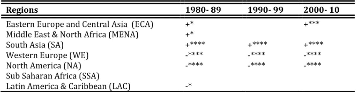
Tables 3 and 4 provide a synthesis of the domestic efforts towards environmental protection (DEEP) of different groups of countries over the periods 1980-1989,

3 _{The real exchange effective rate (REER) is computed by taking into account oil exporters in the} calculation of the weighting of the main trade partners. When we use the REER without oil exporters ant the volatility of real exchange effective rate, we find similar results.

15 1999 and 2000-2010. We may distinguish three groups. The first groups (Eastern Europe and Central Asia (ECA) and South Asia (SA)) are countries in which domestic efforts towards environmental regulation are weak. These domestic efforts do not compensate for structural environmental degradation (carbon dioxide emissions) over the three decades (1980-1989, 1990-1999 and 2000-2010). Similar results are found for the second group (Middle East & North Africa (MENA)) even if these domestic policies have no effect on environmental degradation during the period 2000-2009 and 1990-1999 respectively. The third group (North America (NA), Western Europe (WE)) are countries which have domestic policies that appear to be successful in reducing environmental degradation.

Annex 1 shows that the two indicators (domestic efforts of environmental protection) are correlated to multilateral environmental agreements (such as Annex 1 of Kyoto Protocol) and some environmental measures such as energy taxes (Energy tax revenues as a percentage of total revenues) and environmental tax ratios.

16

Table 2: Estimation Results (Carbon dioxide emissions and Sulphur dioxide emissions) Dependent variables Log of carbon dioxide per capita Log of sulphur dioxide per capita

(1) (2) (3) (4) (5) (6)

Lagged carbon dioxide 0.656*** 0.894*** 0.593*** per capita (log) (4.930) (8.955) (5.070)

Lagged sulphur dioxide 0.970*** 1.043*** 0.754***

per capita (log) (6.907) (8.770) (4.839)

Income capita (log) 0.404*** 0.208*** 1.649** 0.241*** 0.173*** 2.920***

(3.167) (3.135) (2.474) (3.080) (3.613) (2.749) Population growth 0.0456* -0.00713 -0.00961 -0.00581 0.0758 0.250** (1.692) (-0.170) (-0.182) (-0.0801) (0.833) (2.091) Economic growth 0.0174*** 0.0362*** 0.0187*** 0.0145** 0.0371** 0.00540** (3.041) (4.593) (3.721) (2.054) (2.605) (2.045) Trade (log) 0.0921** 0.0708*** 0.0860** -0.599* -0.588 -0.0532 (2.006) (2.934) (2.283) (-1.731) (-1.423) (-0.154) REER -0.145 -0.501** (-1.573) (-2.059) Income inequality -0.0456* -0.0160** -0.0174*** -0.0168* (-1.692) (-2.028) (-3.041) (-1.704)

Income cap sq (log) 0.0128 -0.178***

(0.239) (-2.787) Intercept -1.395* -1.503** -6.592** 4.145** 4.132** -13.34** (-1.798) (-2.350) (-2.413) (2.118) (2.179) (-2.316) Observations 689 486 486 554 389 389 Countries 128 111 111 124 107 107 AR(1) 0.004 0.016 0.01 0.058 0.062 0.001 AR(2) 0.396 0.364 0.443 0.128 0.568 0.384 Hansen Test 0.269 0.432 0.163 0.166 0.176 0.176 Instruments 25 24 25 24 21 22

Notes: * significantly at 10%; ** at 5%; *** at 1%. The study period is 1980-2010 and 1980-2004 for carbon dioxide emissions and sulphur dioxide emissions respectively. For robustness checks we include other variables (the density of population, natural resources, oil and minerals rents). They do not have an effect on environmental degradation.

17 Table 3: Index of Domestic Efforts for environmental protection: CO2 emissions

Regions 1980- 89 1990- 99 2000- 10

Eastern Europe and Central Asia (ECA) +* +***

Middle East & North Africa (MENA) +*

South Asia (SA) +**** +**** +****

Western Europe (WE) -**** -**** -****

North America (NA) -**** -**** -****

Sub Saharan Africa (SSA)

Latin America & Caribbean (LAC) -*

The signs are reported here when they are statistically different from zero at the 1% (****), 5% (***), 10%level (**), and 25% (*) levels. Negative signs are for successful environmental policies

Table 4: Domestic Efforts for environmental protection: SO2 emissions

Regions 1980-89 1990-99 2000-04

Eastern Europe and Central Asia (ECA) +* -**** Middle East & North Africa (MENA) +****

South Asia (SA) -* -****

Western, Europe (WE) -* -**** -*

North America (NA) -* -****

Sub Saharan Africa (SS) -**** -*

Latin America & Caribbean (LAC) -***

The signs are reported here when they are statistically different from zero at the 1% (****), 5% (***), 10% (**), 25% (*) levels

18

19

20

4

Empirical analysis: effect of revealed environmental policies on

bilateral trade

The objective of the paper is to analyse the effect of gaps in environmental policies between trading partners on bilateral trade flows for the period 1980-2010. For this purpose, we present the econometric model and the empirical method. Moreover, we describe the determinants of bilateral trade flows and the database source.

4.1 Empirical Model 4.1.1 Econometric model

In line with previous papers, we use an augmented gravity model of international trade. The gravity model relates bilateral trade flows (exports) between country i and country j at time t to its determinants (such as the economic sizes, trade costs, environmental policies). The equation can be written as:

ln , , = + + , + + + , , + + ε, , (5)

With the matrix of control variables, _{, ,} is the gap in environmental policies between trading partners (i, j) at period t. The gap in environmental policies is the absolute difference of domestic efforts for environmental protection (DEEP) of the exporting and importing countries. The data cover the period from 1980 to 2010 and are compiled in five-year averages (1980-1984, 1985-1989…). _{, ,} is the export flow from country (i) to country (j) at period (t).

Control variables ( ) are the main determinants of bilateral trade flows. They are the distance between country i and country j, the existence of a common border (the variable is equal to one if i and j share a common border), the language (an index of language similarity between countries i and j)4_{; the economic and population size of}

partner countries, and the real exchange effective rate of countries. These are from the economic literature. Finally ε_{, ,} is the error term. The model also includes a complete set of specific effects:

4 _{The fixed effect estimates with country-pair takes bilateral distance, colonial linkages, common border} into account.

21 : common effect to all periods and pairs of countries (constant)

: specific effect to periods t but common to all the pairs of countries to take into account common shocks . _,

, : specific effect to each pair of countries and common to all the periods.

: exporter specific effect and and importer specific effect 4.1.2 Estimation strategy

The effect of domestic environmental policies on bilateral trade is tested with a panel gravity model framework. Equation (1) can be estimated with three basic approaches: ordinary least square (OLS), fixed effects (FE) or random effects (RE).

The main disadvantage of using OLS estimates is that they do not take into account any unobserved heterogeneity of countries which simultaneously affects the environmental policies and the volume of trade. Indeed, Anderson & van Wincoop (2003) highlighted the existence of multilateral resistance among trading partners.The

OLS estimates may be biased if the equation does not specifically take the unobserved

heterogeneity of countries into account. To control for multilateral resistance among

trading partners, we follow previous studies (Yu 2010; Carrère 2006) and include

country-pair specific effects. They control for bilateral distance, colonial linkages,

common borders, or any other geographical or time-invariant institutional characteristics. They may be determinants of bilateral flows as evidenced in previous empirical studies (Carrère 2006; Baier & Bergstrand 2007; Baier & Bergstrand 2009). The Hausman test allows a choice of fixed effects (FE) versus random effects (RE).

4.2 Data sources and description of variables

Bilateral exports flows are from the UN Comtrade database for the period 1980-2010. The dataset has 72 export and 128 import countries. Income (GDP) and the population of each home and host country are drawn from the World Development Indicators (2012). The data on distance, contiguity and cultural proximity (common language) are from the CEPII distance database. The data on real effective exchange rate (REER)5 _are

from CERDI. The index of environmental policy is the residual of regression in which environmental quality (carbon dioxide per capita) is explained by structural and mixed factors (see Table 1). We compute our index, labelled domestic effort for environmental

22 protection (DEEP), by normalizing the residual of regression. We obtain a score ranging from -10 (stringent DEEP) to 10 (laxist DEEP).

Appendix 2 presents the definition and source of variables whereas descriptive statistics and correlation of variables are summarized in Appendix 3, 4, 5 and 6.

5

Results

5.1 Basic results

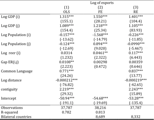
Table 5 gives the results of the effects of gaps in revealed environmental policies (domestic effort for environmental protection) between partner countries on trade flows, using different econometric methods. Column (1) presents the results with an OLS estimator. It allows traditional determinants of trade flows such as common language, distance, common language and contiguity to be taken into account. It does not, however, take the unobserved heterogeneity of countries into account. We thus run fixed effects (column 2) and random effects (column 3) estimators.

Most determinants are significant and consistent with expectations. The higher the income of both exporting and importing countries, the larger the trade flow. In other words, income captures the increasing capacity of partner countries to trade. Trade flows reduce with the population size of partner countries because bigger countries have relatively lower costs when trading domestically than do smaller ones, and may benefit from increasing returns.

The increase of distance between partner countries has a negative effect on trade flow whereas countries that share a common border and common language trade more. Indeed a common border and language may reduce transaction costs and facilitate trade negotiations. An appreciation of real effective exchange rate increases trade flows. This result does not conform to economic theory. Indeed, an increase of REER reflects an appreciation of the exporting country’s currency against its main trading partners, which reduce exports.

Whatever the method used, results show that a gap in environmental policies has no effect on bilateral trade flows. Indeed the coefficient associated with a gap in environmental policies is not significant. It suggests neither pollution havens nor evidence

23 for the Porter hypothesis, which would be reflected, respectively, in significant positive and negative coefficients for environmental policies. Two arguments may partially explain our results. First, we may assume that the costs of domestic environmental policies are low compared to other factors (economic size, endowments, technology, transports, etc). Secondly, we may consider that the potential effect of environmental policies may depend on the nature or the type or characteristic of the goods. Indeed more stringent environmental regulation may only have an effect on specific goods, such as energy intensive goods.

Table 5: Effect of similarity in environmental policy on bilateral trade flows

Log of exports (1) (2) (3) OLS FE RE Log GDP (i) 1.315*** 1.550*** 1.401*** (155.1) (28.21) (104.4) Log GDP (j) 1.089*** 1.218*** 1.105*** (154.4) (25.34) (83.93)

Log Population (i) -0.157*** -1.568*** -0.226***

(-13.62) (-14.79) (-11.85)

Log Population (j) -0.124*** 0.894*** -0.0990***

(-12.69) (9.020) (-5.467)

Log reer (i) 0.0314 0.0461** 0.117***

(1.232) (2.322) (6.443) Gap ER(i,j) 0.0108** 0.00298 0.00359 (2.223) (0.472) (0.646) Common Language 0.771*** 0.837*** (24.26) (13.77) Log distance -0.000212*** -0.000219*** (-76.82) (-42.65) contiguity 2.219*** 2.243*** (29.32) (15.89) Intercept -50.94*** -54.68*** -53.28*** (-191.1) (-19.69) (-135.4) Observations 37,787 38,216 37,787 R-squared 0.782 0.813 Bilateral countries 8,689 8,332

***, ** and * significant at 1%, 5% and 10% levels. T statistics in parentheses

5.2 Heterogeneity in the levels of economic development and characteristics of goods

In this section, we identify potential heterogeneities in the relationship between gaps in environmental policies and bilateral trade flows. First, we evaluate whether the effect of a gap in environmental policies on trade flows is conditional on the level of

24 development of countries. Second, we focus our attention on the effect of environmental policies on the characteristics of exported goods.

5.2.1 Does economic development matter?

Given that the incomes of trading partners may vary, is the effect of differences in environmental policies on trade flows sensitive to their level of economic development? Indeed we may assume that the marginal effect of a gap in environmental policies could be stronger in some countries than in others. When the level of economic development of trading partners increases, they may be incited to increase domestic efforts towards environmental protection. We test this hypothesis by adding in our estimations the level of economic development of trading partners (GDP, column 2, table 6), the difference in economic development of trading partners (column 3, table 6) and their interactive term (gap in environmental policies*GDP of trading partners, gap in environmental policies*difference in GDP of trading partners). Results show that the impact of a gap in environmental policies on trade flows is not conditional on the level or difference in economic development of trading partners.

5.2.2 Do the characteristics of products have an effect?

By increasing the costs of firms through abatement policies or environmental tax, environmental policies may increase prices and reduce the competitiveness of goods. However the sensitivity of consumers to price variation depends on the nature of goods. They may be more sensitive to differentiated goods than homogeneous goods. To take into account the characteristics of goods, we distinguish manufactured goods (column 3 of table 7) and primary common goods (column 2 of table 7). We find that the marginal impact of a gap in environmental policies does not depend on the characteristics of goods. In other words, it does not favour (or dampen) the export of manufactured and primary commodity products.

25 Table 6: Effect of similarity in environmental policy on bilateral trade flows: the

importance of economic development

Dependent variable Log of exports

(1) (2) (3)

Log GDP (i) 1.550*** 1.555*** 1.549***

(28.21) (28.11) (28.05)

Log GDP (j) 1.218*** 1.222*** 1.217***

(25.34) (25.28) (25.23)

Log Population (i) -1.568*** -1.575*** -1.567***

(-14.79) (-14.81) (-14.76)

Log Population (j) 0.894*** 0.890*** 0.895***

(9.020) (8.975) (9.022)

Log reer (i) 0.0461** 0.0453** 0.0463**

(2.322) (2.280) (2.329)

Gap ER(i,j) 0.00298 0.0792 -0.0118

(0.472) (0.871) (-0.165)

Gap ER(i,j)*Log GDP -0.00306

per capita (i,j) (-0.840)

Gap ER(i,j)*Difference in log GDP 0.000587

per capita (i,j) (0.207)

Intercept -54.68*** -54.75*** -54.67***

(-19.69) (-19.71) (-19.68)

Observations 38,216 38,216 38,216

R-squared 0.813 0.813 0.813

Joint signif Gap ER(i,j) coeff (p-value) 0.4007 0.8754

Bilateral countries 8,689 8,689 8,689

26 Table 7: Environmental policies and trade flows: characteristics of

goods (manufactured and primary commodity)

Dependent variable Exports (log) Primary commodity exports (log) Manufactured exports (log) (1) (2) (3) Log GDP (i) 1.550*** 0.748** 2.001*** (28.21) (2.569) (6.323) Log GDP (j) 1.218*** 0.986*** 1.044*** (25.34) (7.327) (6.534)

Log Population (i) -1.568*** -1.802*** 0.821

(-14.79) (-2.610) (1.480)

Log Population (j) 0.894*** -0.925*** -0.759**

(9.020) (-3.660) (-2.374)

Log reer (i) 0.0461** -0.455 0.370

(2.322) (-1.193) (1.282) Gap ER(i,j) 0.00298 0.00658 0.00137 (0.472) (0.323) (0.0576) Intercept -54.68*** 11.16 -69.45*** (-19.69) (0.883) (-5.966) Observations 38,216 1,777 3,046 R-squared 0.813 0.307 0.188 Bilateral countries 8,689 465 897

***, ** and * significant at 1%, 5% and 10% levels. T statistics in parentheses

5.3 Robustness Checks

Previous sections show that a similarity in environmental policies between trading partners has no effect on their trade flows. We verify the robustness of previous results in several ways. First, we include more control variables to check the pertinence of results. Second, we apply an alternative econometric approach, the Poisson pseudo-maximum likelihood (PPML) estimation to address the zero trade problem. Third, we use other measures of bilateral trade and environmental policies.

5.3.1 Adding control variables

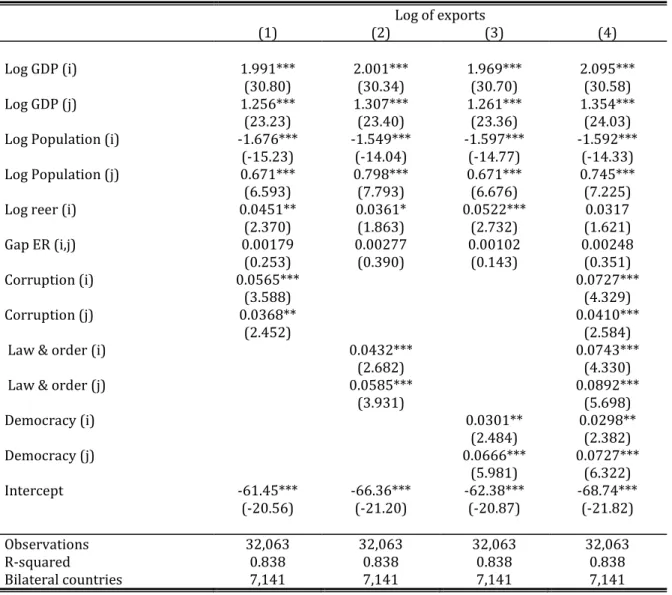
Previous results have shown that the similarity in environmental policies between trading countries has no effect on bilateral trade flows. However environmental policy could be a reflection of the quality of institutions. In other words, the stricter a country’s environmental policy, the better institutions it will have. Indeed some authors (Méon & Sekkat 2008; Yu 2010) suggest that institutions could promote trade flows, particularly for manufactured goods. This may explain the non-significance of the interest variable. In order to capture the effect of environmental policies only, we control for institutional quality and include the level of corruption, the quality of law and order and democracy

27 in trading partners. The results are not affected (Table 8) when controlling either by corruption, order and law and democracy.

Table 8: Effect of similarity in environmental policy on bilateral trade flows: more control variables Log of exports (1) (2) (3) (4) Log GDP (i) 1.991*** 2.001*** 1.969*** 2.095*** (30.80) (30.34) (30.70) (30.58) Log GDP (j) 1.256*** 1.307*** 1.261*** 1.354*** (23.23) (23.40) (23.36) (24.03)

Log Population (i) -1.676*** -1.549*** -1.597*** -1.592***

(-15.23) (-14.04) (-14.77) (-14.33)

Log Population (j) 0.671*** 0.798*** 0.671*** 0.745***

(6.593) (7.793) (6.676) (7.225)

Log reer (i) 0.0451** 0.0361* 0.0522*** 0.0317

(2.370) (1.863) (2.732) (1.621) Gap ER (i,j) 0.00179 0.00277 0.00102 0.00248 (0.253) (0.390) (0.143) (0.351) Corruption (i) 0.0565*** 0.0727*** (3.588) (4.329) Corruption (j) 0.0368** 0.0410*** (2.452) (2.584)

Law & order (i) 0.0432*** 0.0743***

(2.682) (4.330)

Law & order (j) 0.0585*** 0.0892***

(3.931) (5.698) Democracy (i) 0.0301** 0.0298** (2.484) (2.382) Democracy (j) 0.0666*** 0.0727*** (5.981) (6.322) Intercept -61.45*** -66.36*** -62.38*** -68.74*** (-20.56) (-21.20) (-20.87) (-21.82) Observations 32,063 32,063 32,063 32,063 R-squared 0.838 0.838 0.838 0.838 Bilateral countries 7,141 7,141 7,141 7,141

***, ** and * significant at 1%, 5% and 10% levels. T statistics in parentheses

5.3.2 The problem of zero observations

Recent advances in the economic literature on trade gravity models have shown that there may be large part of zero export flows between partner’s countries. Our previous results are based on a truncated sample because 10% of country-pairs do not trade. They are dropped from estimates when we use logarithms of export flows. We therefore run Poisson pseudo-maximum likelihood (PPML) estimators (Silva & Tenreyro 2006) for which results are reported in column (2) of Table 9. We find that the similarity in environmental policies between trading countries again has no effect on bilateral trade flows.

28 Table 9: Effect of similarity in environmental policy on

bilateral trade flows

Dependent variable Log of exports Export

(1) (2) FE PPML Log GDP (i) 1.550*** 0.765*** (28.21) (13.02) Log GDP (j) 1.218*** 0.883*** (25.34) (22.41)

Log Population (i) -1.568*** -0.0308

(-14.79) (-0.511)

Log Population (j) 0.894*** -0.206***

(9.020) (-5.388)

Log reer (i) 0.0461** 2.982**

(2.322) (2.244) Gap ER (i,j) 0.00298 -0.0269 (0.472) (-1.328) Intercept -54.68*** -39.38*** (-19.69) (-5.599) Observations 38,216 42,292 R-squared 0.813 0.371 Bilateral countries 8,689

***, ** and * significant at 1%, 5% and 10% levels. T statistics in parentheses

5.3.3 Alternative measure of bilateral trade and environmental policies

In the baseline model (equation 5), the dependent variable is the bilateral export flow. Because our sample is a set of heterogeneous countries, we normalize the bilateral export flows and use the ratio bilateral exports to GDP (Vijil & Wagner 2012; Melo & Grether 2000).

In accordance with the modification of the dependent variable, the GDP and Population of partner countries are substituted by GDP per capita. Indeed, according to the literature, economic size may be captured either by a country´s income (GDP) and population or by a country´s income per capita (GDP per capita). We then consider income per capita because the dependent variable (bilateral exports /GDP) is mechanically related to income (GDP). Other traditional determinants are similar. Table

29 10 concludes that a similarity in environmental policies has no effect on bilateral exports, primary commodity exports and manufactured exports.

Two alternative measures of environmental policy are also employed. To make sure that our results are robust, environmental policy is computed with additional mixed variables: income inequality and the square of income per capita (Environmental Kuznets Curve). Whatever the indicator6 _{(Gap ER (i,j)_A, Gap ER (i,j)_B) used, the results}

(Table 11) are always unchanged.

6 _{To compute Gap ER (i,j)_A and Gap ER (i,j)_B, we use columns 2 and 3 of Table 2. We find similar results} when we use DEEP for Sulphur dioxide emissions (columns 4, 5 and 6 of table 2). Tables are available for requests.

30

Table 10: Effect of similarity in environmental policy on bilateral trade (export to GDP ratio)

Dependent variable Log of export Primary

commodity exports (log

Manufactured exports (log)

(1) (2) (3) (4) (5)

Log GDP per capita (i) 0.731*** 1.321*** 0.732*** 0.771*** 1.658***

(13.98) (19.65) (13.90) (2.656) (5.316)

Log GDP per capita (j) 0.896*** 1.339*** 0.896*** 0.963*** 1.001***

(19.56) (24.07) (19.50) (7.735) (6.593)

Log bilateral teer (i,j) 0.108*** 0.113*** 0.108*** -0.171 -0.517**

(5.620) (5.891) (5.610) (-0.503) (-2.201)

Gap ER (i,j) 0.00333 -0.0290 0.00548 0.00574 -0.000185

(0.524) (-0.673) (0.184) (0.282) (-0.00771)

Gap ER(i,j)*Log GDP

per capita (i,j) 0.00358

(0.700)

Log GDP per capita(i,j) -1.654***

(-14.23) Gap ER(i,j)*Difference

GDP(log) per capita (i,j) -0.000256

Gap ER(i,j)*Log GDP per capita (i,j)

(-0.0739) Intercept -36.67*** -31.09*** -36.67*** -6.145** -13.27*** (-67.26) (-45.59) (-66.73) (-2.423) (-5.435) Observations 38,216 38,216 38,216 1,777 3,046 R-squared 0.787 0.788 0.787 0.305 0.177 Bilateral countries 8,689 8,689 8,689 465 897

31 Table 11: Similarity in environmental policy and bilateral trade: alternative

measures of environmental policy

Dependent variable Log of exports

(1) (2) (3)

Log GDP (i) 1.550*** 1.258*** 1.261***

(28.21) (11.82) (11.76)

Log GDP (j) 1.218*** 1.419*** 1.426***

(25.34) (10.89) (10.91)

Log Population (i) -1.568*** -1.415*** -1.438*** (-14.79) (-5.208) (-5.274)

Log Population (j) 0.894*** 1.574*** 1.561***

(9.020) (6.876) (6.817)

Log bilateral teer (i,j) 0.0461** 0.115 0.117

(2.322) (1.305) (1.322) Gap ER (i,j)_A -0.0112 (-1.013) Gap ER (i,j) 0.00298 (0.472) Gap ER (i,j)_B 0.00234 (0.226) Intercept -54.68*** -67.13*** -66.81*** (-19.69) (-9.916) (-9.877) Observations 38,216 10,861 10,861 R-squared 0.813 0.714 0.714 Bilateral Countries 8,689 3,866 3,866

32

6

Conclusion

This paper analyses the effect of a gap in revealed environmental policies between trading partners on bilateral trade flows for 122 countries in the period 1980-2010. Contrary to previous papers in the economic literature, which use either input-oriented indicators or output-oriented indicators, we use an index of environmental policy. Labelled domestic efforts for environmental protection (deep), this index does not depend on other factors (structural or mixed) in that country’s policy.

Our results suggest that a gap in environmental policies does not dampen bilateral trade flows. Second, we show that the effect (absence) of a gap in environmental policies on trade flows is not conditional on the level of development of countries. Third the results don’t depend on the characteristics (manufactured goods and primary commodity) of exported goods. These results are robust to alternative robustness checks.

Our results are important in terms of recommendations for economic policies. They incite developing and developed countries to increase efforts to protect environmental quality. These climate and environmental policies will not dampen the competitiveness of countries.

7

References

Abbas, Mehdi. 2011. « Mondialisation et développement. Quelle soutenabilité au régime de l’Organisation mondiale du commerce? » Mondes en développement (2): 17–28. Acemoglu, Daron, Philippe Aghion, Leonardo Bursztyn, et David Hemous. 2012. « The Environment and Directed Technical Change ». American Economic Review 102 (1) (février): 131‑166. doi:10.1257/aer.102.1.131.

Aichele, Rahel, et Gabriel Felbermayr. 2013. « Estimating the Effects of Kyoto on Bilateral Trade Flows Using Matching Econometrics ». The World Economy 36 (3): 303–330. doi:10.1111/twec.12053.

Albrecht, Johan A. E. 1998. « Environmental Costs and Competitiveness. A Product-Specific Test of the Porter Hypothesis ». SSRN Scholarly Paper ID 137953. Rochester, NY: Social Science Research Network. http://papers.ssrn.com/abstract=137953.

33 Ambec, Stefan, Mark A. Cohen, Stewart Elgie, et Paul Lanoie. 2013. « The Porter Hypothesis at 20: Can Environmental Regulation Enhance Innovation and Competitiveness? » Review of Environmental Economics and Policy 7 (1) (janvier 1): 2‑22. doi:10.1093/reep/res016.

Anderson, James E, et Eric van Wincoop. 2003. « Gravity with Gravitas: A Solution to the Border Puzzle ». American Economic Review 93 (1) (mars): 170‑192. doi:10.1257/000282803321455214.

Antweiler, Werner, Brian R Copeland, et M. Scott Taylor. 2001a. « Is Free Trade Good for the Environment? » American Economic Review 91 (4) (septembre): 877‑908. doi:10.1257/aer.91.4.877.

Antweiler, Werner, Brian R. Copeland, et M. Scott Taylor. 2001b. « Is Free Trade Good for the Environment? » American Economic Review 91 (4): 877‑908.

Arcand, Jean-Louis, Patrick Guillaumont, et Sylviane Guillaumont Jeanneney. 2008. « Deforestation and the real exchange rate ». Journal of Development Economics 86 (2): 242‑262.

Arellano, Manuel, et Stephen Bond. 1991. « Some Tests of Specification for Panel Data: Monte Carlo Evidence and an Application to Employment Equations ». Review of

Economic Studies 58 (2): 277‑97.

Arellano, Manuel, et Olympia Bover. 1995. « Another look at the instrumental variable estimation of error-components models ». Journal of Econometrics 68 (1): 29‑51. Baier, Scott L., et Jeffrey H. Bergstrand. 2007. « Do free trade agreements actually

increase members’ international trade? » Journal of International Economics 71 (1) (mars 8): 72‑95. doi:10.1016/j.jinteco.2006.02.005.

———. 2009. « Bonus vetus OLS: A simple method for approximating international trade-cost effects using the gravity equation ». Journal of International Economics 77 (1) (février): 77‑85. doi:10.1016/j.jinteco.2008.10.004.

Barbier, Edward. 2011. « The Policy Challenges for Green Economy and Sustainable Economic Development ». Natural Resources Forum 35 (3): 233–245. doi:10.1111/j.1477-8947.2011.01397.x.

Blundell, Richard, et Stephen Bond. 1998. « Initial conditions and moment restrictions in dynamic panel data models ». Journal of Econometrics 87 (1): 115‑143.

Borghesi, S. 2006. « 2 Income inequality and the environmental Kuznets curve ».

Environment, inequality and collective action: 33.

Boussichas, Matthieu, et Michael Goujon. 2010. « A quantitative indicator of the immigration policy’s restrictiveness ». Economics Bulletin 30 (3): 1727‑1736. Boyce, J. K. 1994. « Inequality as a cause of environmental degradation ». Ecological

Economics 11 (3): 169–178.

Brock, William, et M. Taylor. 2010. « The Green Solow model ». Journal of Economic