A random walk approach to stochastic neutron transport

HAL Id: tel-01301385

https://tel.archives-ouvertes.fr/tel-01301385

Submitted on 12 Apr 2016

HAL is a multi-disciplinary open access

archive for the deposit and dissemination of sci-entific research documents, whether they are pub-lished or not. The documents may come from teaching and research institutions in France or abroad, or from public or private research centers.

L’archive ouverte pluridisciplinaire HAL, est destinée au dépôt et à la diffusion de documents scientifiques de niveau recherche, publiés ou non, émanant des établissements d’enseignement et de recherche français ou étrangers, des laboratoires publics ou privés.

Clelia De Mulatier

To cite this version:

Clelia De Mulatier. A random walk approach to stochastic neutron transport. Mathematical Physics [math-ph]. Université Paris-Saclay, 2015. English. �NNT : 2015SACLS029�. �tel-01301385�

T

HÈSE DE DOCTORAT

DE

L’U

NIVERSITÉ

P

ARIS

-S

ACLAY

préparée à L’Université Paris-Sud

É

COLE

D

OCTORALE

564

Physique en Île-de-France

Spécialité Physique

par

Clélia de Mulatier

A

RANDOM WALK APPROACH

TO STOCHASTIC NEUTRON TRANSPORT

Thèse soutenue à Orsay le 12 octobre 2015 Composition du Jury :

M. BÉNICHOUOlivier Directeur de recherche CNRS, Université Pierre et Marie Curie Président Mme BURIONIRaffaella Professeur, Università di Parma Rapporteur Mme DULLASandra Professeur, Politecnico di Torino Rapporteur M. GOBETEmmanuel Professeur, École Polytechnique Examinateur M. DIOPCheikh Professeur, CEA Saclay et INSTN Directeur de thèse M. ROSSOAlberto Directeur de recherche CNRS, Université Paris-Sud Co-directeur de thèse

Je profite des ces quelques lignes pour remercier les personnes avec qui j’ai eu la chance de travailler, ceux qui m’ont accompagnée ou encouragée, ou, tout simplement, ceux avec qui j’ai passé de bons moments au cours de ces trois dernières années.

Mes premiers remerciement vont tout droit à Andrea sans qui cette thèse n’aurait pas été ce qu’elle est maintenant. Merci de m’avoir supportée ces trois ans, encouragée, et aidée ; merci pour la confiance que tu m’as ac-cordé sur le plan scientifique et pour ta patience. Enfin, merci d’avoir pris le temps de répondre à mes multiples questions, et de m’avoir donné tout un tas d’équations et de calculs à dériver ! je n’aurais pas appris tant de choses nouvelles sans ton aide, ce sont toutes nos discussions qui m’ont donné envie de continuer dans la recherche. Je suis aussi ravie de ne pas t’avoir découragé et d’apprendre que tu commences l’encadrement d’une nouvelle thésarde.

Je tiens aussi à remercier tout particulièrement mes deux directeurs de thèse. Cheikh, pour sa perspicacité et son expertise en terme de thèse, qui ont fortement contribué à mener à bien cette thèse interdisciplinaire, partagée entre deux laboratoires. Et enfin, Alberto, un grand merci pour m’avoir fait découvrir le domaine de la physique statistique, ainsi que celui de la recherche ! merci de m’avoir guidé depuis le stage de M1, celui de M2, et jusqu’à la thèse. J’ai beaucoup apprécié tous les projets de recherche que tu as pu me proposer. Je me souviens du premier mail que je t’ai en-voyé pour le stage de M1, j’avais peur d’essuyer un refus, jamais je n’aurais imaginé arriver jusqu’ici.

Je souhaite ensuite remercier chaleureusement l’intégralité des mem-bres de mon jury de thèse. I’m very grateful to Sandra Dulla and Raffaella Burioni for the time they have dedicated to carefully reviewing my thesis. I was also very honoured by the presence of Olivier Bénichou and Em-manuel Gobet as jury members. I would like to express my gratitude to the members of my defense committee for their participation to my PhD defense and for the interest they showed for my work.

Je tiens aussi à remercier les différents chercheurs avec qui j’ai eu la chance de collaborer, tout particulièrement Grégory, Alain, Eric et PK. Je suis très reconnaissante envers Grégory pour le temps précieux qu’il a pu m’accorder et les projets enrichissants qu’il m’a proposé.

Merci à Emmanuel Trizac et à Franck Gabriel pour m’avoir accueillie dans vos laboratoires respectifs. En particulier, je suis reconnaissante en-vers Emmanuel Trizac pour m’avoir permis de recevoir des lycéens au LPTMS. Je souhaite aussi remercier les membres du LPTMS et du LTSD pour leurs conseils et le temps qu’ils ont pris pour répondre à mes ques-tions ; merci tout particulièrement à Christophe, Martin, Raoul, Denis, Guil-laume, Mikhail et François-Xavier.

Je tiens aussi à remercier tout particulièrement Claudine pour son or-ganisation, son soutien et sa bonne humeur ! Ainsi que Vincent, ton incroy-able facilité à communiquer avec nos ordinateurs quand nous en sommes complètement incapables m’a sauvée à de nombreuses reprises ! merci aussi pour tous les raccourcis bash que tu as pu m’apprendre. echo -e "\xf0\x9f\x8d\xba" ! Merci Thérèse pour l’attention que tu m’as accordé, tes conseils et les diverses discussions entre deux arrêts de RER B tardifs.

La thèse n’a pas seulement été axée sur la recherche, mais m’a aussi permis de passer de bons moments de « détente » en cours ! Merci aux enseignants et collègues avec qui j’ai eu la chance de travailler, Daniel, Na-dia, François, Hervé, Corinne et Julien. J’ai énormément apprécié enseigner pour vos cours. Un grand merci aux étudiants, avec qui j’ai passé de super moments !

La thèse, c’est aussi de très bons moments passés entre thésards/étu-diants/postdoc. Je pense tout particulièrement à Andrey, Andrii, François, Giulia, Ricardo, Pierre, Vincent, Yasar, Karim, Cyril, Arthur, Olga, France, Ben, RiCyl, et les bonhommes LEGO® ! Merci beaucoup Cyril pour avoir pris le temps de relire et commenter une partie de mon manuscrit, et pour m’avoir partagé ta passion pour la physique des réacteurs. Merci à Kevin, Olga, Ricardo et Pierre pour les divers problèmes passionnants de physique ou math sur lesquels nous avons pu échanger. J’ai beaucoup aimé nos dis-cussions, et j’espère bien avoir encore de nombreuses occasions.

Je pense aussi à tous ces amis avec qui j’ai passé de très bons moments ces dernières années; un grand merci à la coloc’du 14e, Vivien, Émilien, Cécile, Grégoire, sans qui la thèse n’aurait pas été aussi sympathique, et à mes coloc’ de fin de thèse Kar’ et Pierre (!) ; et aux amis de longue date, qui m’ont conseillée et soutenue, Marine, Thibaut, Sylvain, Antoine, Jules,. . .

Marine, merci pour nos nombreux bavardages, ton grand talent et tes con-seils de psychologue !

Mes derniers remerciements vont tout droit à ma famille « adorée », mes parents qui m’ont toujours accompagnée ; et mes frères et sœurs, Geo (merci de m’avoir aidée à percer le mystère du fonctionnement des ascenseurs !), ma chroutt’ adorée (j’attends ta thèse avec impatience ! ;p ), Hortichou (merci à toi de continuer à nous faire tant rêver de musique) et J-T (je sais, c’est Jean-Théophane ! ahhh, heureusement que tu es là !).

Ma dernière pensée va à Eugenio. Aussi paradoxal que cela puisse être, je suis pleine de gratitude envers ces trois années de doctorat qui m’ont permis de te rencontrer, tout comme je te remercie de m’avoir tant soutenue pour les terminer. (turtle) ! Merci pour ta patience, ta gentillesse, et tous ces instants de bonheur que tu me fais vivre.

CONTRIBUTIONS DE LA THÉORIE DES MARCHES ALÉATOIRES AU TRANSPORT STOCHASTIQUE DES NEUTRONS

Au cours de mon doctorat, j’ai effectué mon activité de recherche sous la codirection d’Alberto Rosso au LPTMS (Université Paris-Sud - CNRS) et de Cheikh Diop et Andrea Zoia au LTSD (CEA Saclay DEN/DM2S/SERMA). Cette double affiliation m’a permis de travailler à l’interface de la physique statistique et de la physique des réacteurs nucléaires. Je me suis plus spé-cifiquement intéressée aux propriétés des marches aléatoires branchantes et de la diffusion anormale dans le contexte du transport stochastique des neutrons au sein d’un réacteur nucléaire. En outre, quelques-uns des as-pects originaux de la thèse sont l’étude des fluctuations statistiques – spa-tiales et temporelles – de la population de neutrons et le travail en géome-trie confinée ou en présence de bords (prise en compte des bords du sys-tème). Ce travail, réalisé en collaboration avec différents chercheurs du LTSD et du LPTMS, et rapporté dans ce manuscrit, a donné lieu à plusieurs publications dans des revues internationales. Vous en trouverez ici un court résumé en français.

INTRODUCTION

L’

UN des principaux objectifs de la physique des réacteurs nucléaires est de caractériser la répartition de la population de neutrons au sein d’un réacteur. Due à la nature stochastique des interactions entre ces neu-trons et les noyaux fissiles composant le coeur du réacteur (combustible), cette répartition fluctue spatialement et temporellement. Pour autant, pour la majeur partie des applications en physique des réacteurs, la population de neutrons considérée est très importante – on peut citer par exemple la densité de neutrons au sein d’un réacteur de type REP à pleine puissance en conditions stationnaires qui est de l’ordre de 108_{neutrons par centimètre}

cube. Dans ces conditions, les grandeurs physiques caractérisant le sys-tème (tels que flux, taux de réaction, énergie déposée) sont, en première approximation, bien représentées par leurs valeurs moyennes respectives, qui obéissent à l’équation de transport linéaire de Boltzmann. Cette ap-proche cependant présente des limites : nous nous intéressons ici à deux aspects du transport des neutrons qui ne sont peuvent pas être décrits par cette équation.

Chapitre 1 - Transport des neutrons et physique statistique

Ce chapitre introductif présente le contexte général du transport des neu-trons en physique des réacteurs et explicite le lien avec la physique statis-tique, plus précisément la théorie des marches aléatoires. Dû à la nature stochastique et markovienne des intéractions des neutrons avec les noyaux fissiles du milieu – diffusion, capture stérile, ou encore émission d’un ou plusieurs neutrons lors de la fission d’un noyau – le transport des neutrons au sein d’un matériau fissile peut etre modélisé par des marches aléatoires exponentielles branchantes.

Sont introduits ensuite les notations utilisées dans la thése, ainsi que les observables principales en physique des réacteurs, la densité neutron-ique, le taux de réaction et le flux neutronique. Les équations de bases de la neutronique sont ensuite re-dérivées : l’équation de transport linéaire de Boltzmann sous forme intégro-différentielle et sous forme intégrale, et l’équation de diffusion des neutrons. Ces équations décrivent le comporte-ment des grandeurs moyennes, que sont la densité neutronique, le flux ou le taux de réactions, c.à.d. le comportement moyen de la population de neutrons. Bien qu’adaptée à la plupart des situations en physique des réac-teurs, cette approche présente cependant des limites.

Tout d’abord, elle ne permet pas caractériser les fluctuations statistiques de la population de neutrons, qui peuvent devenir importantes dans des

systèmes où la densité de neutrons est initialement faible. Dans un réacteur REP au démarrage par exemple, la population est initialement faible; des simulations numériques Monte-Carlo réalisées avec le code TRIPOLI-4 au LTSD ont mis en évidence la formation d’amas de neutrons dispersés dans de tels systèmes. Ce comportement surprenant, que nous avons baptisé « clustering neutronique » [Dumonteil et al. 2014], résulte de larges fluctua-tions spatiales et temporelles de la population de neutron, et ne peut donc pas être expliqué à partir des équations de transport usuelles.

D’autre part, l’équation de Boltzmann caractérise le transport des neu-trons dans des milieux où les positions des centres de diffusion (noyaux fissiles) sont non corrélés, c.à.d. dans lesquels le transport des neutrons est de forme exponentiel. Cependant, pour quelques applications, le milieu traversé par les neutrons est fortement hétérogène, voire désordonné (à dé-sordre figé), de sorte que l’hypothèse de centres de diffusion non corrélés n’est plus valide. Citons par exemple le cas des réacteurs à lit de boulets, ou encore le transport radiatif dans des tissus (peau). Pour ce type de milieux, il a été observé que le transport n’obéit plus à un transport simplement exponentiel, et les équations usuelles de la neutronique ne sont alors plus valables.

Le présent manuscrit s’intéresse à ces deux aspects du transport des neutrons non décrit par l’équation de transport linéaire de Boltzmann. La première partie du manuscrit traite des fluctuations statistiques de la popu-lation de neutrons, et plus particulièrement du clustering neutronique. La deuxième partie se concentre sur le transport non-exponentiel, et s’intéresse plus spécifiquement à des propriétés du transport anormal dans un sys-tème de taille fini ou en présence de bords du syssys-tème.

PARTIEI - STATISTIQUES DES FLUCTUATIONS

Nous étudions, dans un premier temps, à un aspect souvent négligé des processus de diffusion avec branchements : les fluctuations statistiques – temporelles et spatiales – de la population de particules. Due au processus de naissances (fissions) et de morts (absorption) de particules, appelé pro-cessus de Galton-Watson, l’amplitude de ces fluctuations croît au cours du temps, jusqu’à devenir comparable au quantités moyennes caractérisant le système (telles que la densité de particules par exemple). Ainsi, même un système critique, pour lequel le taux de naissance est égale au taux de mort (comme c’est le cas pour le fonctionnement d’un réacteur), peut voir sa population disparaître au bout d’un certain temps1_{. Ce phénomène est}

1_{Le temps caractéristique correspondant est bien entendu d’autant plus long que la}

connu en neutronique sous le nom de catastrophe critique [Williams 1974]. Ces fluctuations peuvent-elles conduire à la formation d’amas de neutrons, tels que ceux observés lors des simulations TRIPOLI-4 de réacteurs au dé-marrage, en dépit du fait que ces particules n’interagissent pas directement entre elles ?

Chapitre 2 – Description backward des fluctuations

Ce premier chapitre développe les outils nécessaires à l’étude des fluctua-tions de la population de neutrons. En particulier, nous nous intéressons à deux observables principales (celles d’intéret en physique des réacteurs) : la longueur totale parcourue et le nombre total de collisions effectuées, par une famille de neutrons dans un volume donné du milieu fissile. Les moyennes respectives de ces deux observables sont directement reliées au flux neutronique et au taux de réaction dans le volume considéré. L’étude des moments d’ordre supérieur de ces observables permet d’accéder aux fluctuations statistiques des grandeurs physiques d’intérêts caractérisant la population de neutrons en physique des réacteurs.

Dans ce but, nous avons utilisé le formalisme backward de Feynman-Kac afin de dériver l’équation backward gouvernant la fonction génératrice des moments pour chacune de ces deux observables. Pour se faire, nous nous sommes placés dans le cas le plus général d’un système composé d’un milieu hétérogène, où la diffusion des neutrons peut être anisotrope et les vitesses (énergies) des neutrons peuvent changer à chaque collision [

SNA-MC 2013].

Enfin, nous nous intéressons à la statistique d’occupation des neutrons dans un volume donné de milieu fissile. L’observable considérée est alors le nombre total de neutrons présents dans le volume à un instant t donné2_.

Nous retrouvons alors les équations de Pàl-Bell connues en physique des réacteurs.

Chapitre 3 – Clustering neutronique

Ce chapitre commence par un état de l’art des résultats sur le phénomène de clustering, qui a déjà été observé dans différents domaines et étudié pour des systèmes de "taille infinie". Nous remarquons que la formation des clusters résulte d’une compétition entre le processus de naissance et de mort, qui tend à créer des amas de particules appartenant à la même

2_{Par la suite, nous nous intéresserons de nouveau à cette observable afin de caractériser}

la fonction de corrélation entre paires de particules du système, centrale pour comprendre le phénomène de clustering.

famille, et le processus de diffusion, qui tend à les disperser.

Pour la suite, nous nous concentrons sur les systèmes critiques, qui correspondent aux conditions de fonctionnement des réacteurs nucléaires. Dans ce contexte, nous étudions l’impact de la prise en compte des bords du système (système de volume fini) sur le phénomène de clustering. Puis nous investiguons l’impact d’un processus de contrôle de la population globale de neutrons, tel que celui réalisé par les barres de contrôle au coeur du réacteur. Pour cela nous nous sommes intéressés à la fonction de cor-rélation de paire du système, pour laquelle nous obtenons les équations d’évolution en utilisant une description "backward" du transport des neu-trons.

Nous observons la présence de deux types de fluctuations [Zoia et al. 2014] : a) des fluctuations locales résultant d’une compétition entre le pro-cessus de reproduction/mort qui tend à créer des amas et le propro-cessus de diffusion qui tend à mixer les particules sur l’ensemble du système en un temps caractéristique ⌧D ; b) des fluctuations globales qui mènent

finale-ment l’ensemble de la population à extinction sur un temps caractéristique ⌧E(clustering "trivial" et catastrophe critique). L’ajout d’un processus de

con-trôle de la population totale de neutrons (feedback) permet de bloquer ces fluctuations globales et de prévenir ainsi l’extinction du système (et le clus-tering trivial). On s’intéresse alors aux clusters "stabilisés" (dus aux fluc-tuations locales uniquement), pour lesquels nous calculons la taille carac-téristique. Celle-ci dépend du ratio ⌧E/⌧D, c.à.d. de la compétition entre le

processus de reproduction/mort qui tend à la réduire, et celui de diffusion qui tend à l’augmenter [de Mulatier et al. 2015].

Dans ce chapitre, nous avons approximé le transport des neutrons par un transport Brownien. En perspective, il pourrait être intéressant de con-sidérer une modélisation plus réaliste du système, notamment l’impact des hétérogénéités ou de la dépendance en énergie, ou encore des neutrons re-tardés sur le clustering.

PARTIEII – TRANSPORT ANORMAL

Dans cette seconde partie, nous nous intéressons au transport non-exponentiel des neutrons, initialement motivés par le problème du trans-port dans des milieux fortement hétérogènes et désordonnés, tels que le coeur d’un réacteur à lit de boulets.

Chapitre 4 – Opacité d’un milieu

Certaines des propriétés physiques d’un milieu immergé dans un flot de particules sont étroitement liées à la statistique des trajectories aléatoires effectuées par les particules qui le traversent. Citons par exemple l’opacité d’un milieu, qui peut être définie comme le rapport entre la longueur totale moyenne3 _{parcourue par le flot de neutrons au sein du volume et le libre}

parcourt moyen des neutrons dans le milieu. Plus le flot intéragit avec le milieu, plus ce milieu est considéré comme opaque. La formule d’opacité, connue en neutronique, exprime simplement la longueur totale moyenne parcourue par les neutrons comme proportionnelle au ratio du volume V et de la surface S du milieu.

Il s’agit là d’un résultat connu sous le nom de propriété de Cauchy, qui est vérifiée pour toute marche aléatoire exponentielle branchante critique : la longueur moyenne hLi parcourue par une telle marche au travers d’un domaine de taille finie dépend uniquement des propriétés géométriques du domaine, hLi = ⌘dV/S, où ⌘dest une constante dépendant de la dimension.

Dans ce chapitre nous montrons que la propriété de Cauchy (et donc la formule d’opacité) reste valide dans le cas d’un transport anormal.

Propriété universelle de marches aléatoires de Pearson en géométrie confinée En collaboration avec A. Mazzolo, nous avons caractérisé la statistique d’occupation de marches aléatoires branchantes de Pearson en géométrie confinée, pour une loi de sauts quelconque4_{(sous la condition que la loi}

ad-mette un libre parcours moyen). Nous avons montré que l’ensemble de ces marches vérifient une même propriété, la longueur totale moyenne passée par ces marches dans un domaine de taille fini ne dépend que du ratio du volume sur la surface du domaine, et que cette propriété est en réalité lo-cale [Mazzolo et al. 2014;De Mulatier et al. 2014].

Chapitre 5 – Vols de Lévy asymétriques en présence de bords absorbants (système non confiné)

Dans ce chapitre, nous considérons un marcheur évoluant à une dimension, effectuant des sauts successifs indépendants et identiquement distribués suivant une loi de probabilité asymétrique avec des queues en loi de puis-sance (vol de Lévy asymétrique). En particulier, nous nous intéressons à la probabilité de survie et à la statistique d’occupation d’un tel marcheur en présence de bords absorbants.

3_{Observables introduites au chapitre 2} 4_{y compris en loi de puissance}

En l’absence de bords, la fonction de densité de probabilité des posi-tions du marcheur converge, après un grand nombre de sauts, vers une loi asymétrique stable (de Lévy) dont toutes les caractéristiques sont connues grâce au théorème central limite généralisé.

En présence de bords absorbants, ce théorème ne s’applique plus. La fonction de densité de probabilité des positions du marcheur est alors plus complexe à calculer. En collaboration avec G. Schehr, et par la suite P. K. Mo-hanty, j’ai travaillé sur la détermination des paramètres caractérisant la queue de cette densité de probabilité (c.à.d. loin des bords du système)

[De Mulatier et al. 2013]. Nous caractérisons aussi la probabilité de survie

du marcheur, par le biais du calcul de son exposant de persistance. En-fin quelques pistes sont explorées quant à la généralisation en dimension supérieure.

I

NTRODUCTION

Chapter I A STATISTICALMECHANICSAPPROACH TOREACTORPHYSICS

1 Neutron Transport in Reactor Physics

I.1.1 Neutron as a Point Particle . . . 7

I.1.2 From Neutron Transport in Multiplying Media to Branch-ing Exponential Flights . . . 11

I.1.3 Characterisation of the neutron population: phase space densities . . . 20

2 Boltzmann Equation for Neutron Transport I.2.1 Integro-differential Transport Equation . . . 24

I.2.2 Delayed Neutrons . . . 29

I.2.3 Boundary and Initial Conditions . . . 31

I.2.4 Integral Transport Equation . . . 33

I.2.5 Diffusion Equation . . . 40

3 Limits of the Transport Equation I.3.1 Fluctuations Problem . . . 44

I.3.2 Non Exponential Transport . . . 46

F

LUCTUATION

S

TATISTICS

50

Chapter II BACKWARDDESCRIPTION OF THE FLUCTUATIONS 1 The Fluctuation Problem II.1.1 Useful combinatorial quantities . . . 54

II.1.2 The Birth and Death Process . . . 55

II.1.3 Limits of the usual transport equations to describe fluctuations . . . 59

2 Feynman-Kac Backward Equations

II.2.1 “Backward” quantities . . . 63 II.2.2 Feynman-Kac formalism . . . 67 II.2.3 Comments on the form of the equation . . . 74

3 Quantities of Interest in Reactor Physics

II.3.1 Numerical simulation for the travelled length statistics 76 II.3.2 Collision Statistics . . . 78 II.3.3 Occupation Statistics: Escape, Survival and

Extinc-tion Probability . . . 80 II.3.4 Conclusion and perspectives . . . 84

Chapter III NEUTRON CLUSTERING

1 About the process

III.1.1 A prototype model of a nuclear reactor . . . 90 III.1.2 Elementary clustering with zero-dimensional systems 91

2 Free population

III.2.1 General considerations - Pair Correlation Function . 93 III.2.2 System of Infinite Size . . . 94 III.2.3 System of finite size - Feynman-Kac backward

for-malism and general solution . . . 99 III.2.4 System of finite size - reflecting and absorbing

bound-aries . . . 107

3 Controlled population in a system of finite size

III.3.1 The model . . . 116 III.3.2 Genealogy - the last common ancestor . . . 118 III.3.3 Pair correlation function - Controlled clustering . . . 125 III.3.4 Average squared distance and typical size of a cluster 134

4 Conclusions and perspectives

A

NOMALOUS

T

RANSPORT

138

Chapter IV OPACITY OFBOUNDEDMEDIA

1 Opacity Formulae - Motivation and State of the Art

2 Cauchy Formula for a non-stochastic heterogeneous medium 3 A Universal Property of Branching Random Walks in

Con-fined Geometries

IV.3.2 Integral Equations . . . 156 IV.3.3 A universal and local version of the Cauchy formulae 163 IV.3.4 Ensuing results . . . 166

4 Geometrical Proof for Pearson Random Walk

IV.4.1 Introduction . . . 168 IV.4.2 Geometrical proof . . . 169

5 General Conclusion and Perspectives

Chapter V ASYMMETRIC LÉVY FLIGHTS IN THE PRESENCE OF AB

-SORBING BOUNDARIES

1 Free walker

2 One dimensional Lévy flight with an absorbing boundary at the origin

V.2.1 Survival Probability and Persistence Exponent . . . . 186 V.2.2 Tail of the Propagator . . . 190 V.2.3 Details of the numerical simulation details . . . 193

3 Two dimensional Lévy flights in the presence of absorbing boundaries

V.3.1 General setup . . . 197 V.3.2 Domain D open along x or z . . . 200 V.3.3 Domain D open in an other direction . . . 206

4 Conclusion

RANDOM WALKS ON QUENCHED DISORDERED MEDIA AND OPEN PROBLEM

C

ONCLUSION

A

PPENDIX

221

I

NDEX

244

O

NEof the key goals of nuclear reactor physics is to determine the dis-tribution of the neutron population within a reactor core. This pop-ulation indeed fluctuates in space and time due to the stochastic nature of the interactions between the neutrons and the nuclei of the surround-ing medium. For most applications in reactor physics though, the neutron population considered is very large. For instance, in standard light-water reactors (LWR) at operating condition, the typical neutron density within the reactor core is about 108_{neutrons per cubic centimeter. In these cases,}

all physical observables related to the behaviour of the population, such as the heat production due to fissions, are well characterised by average val-ues, which are governed by the classical linear neutron transport equation, called Boltzmann equation.

However there exist some situations for which a description based on averaged observables provides a misleading characterisation of the behaviour of the neutron population. For example, during the start-up of a LWR, the neutron population is rather small. For such a low-density configuration, numerical investigations, performed with the Monte Carlo TRIPOLI-4 code at the LTSD5_{, have highlighted a peculiar behaviour of the}

neutrons, which spontenously form clusters of highly grouped particles with empty regions in between. This phenomenon, named “neutron clus-tering” [Dumonteil et al. 2014], results from strong fluctuations in space and time of the population. As a consequence, average quantities become insufficient to characterise the system: neutron clustering can not be ex-plained using the mean-field Boltzmann equation.

These strong fluctuations are in fact intrinsic to the process that govern the neutron transport in the phase space, resulting from the interplay of three fundamental mechanisms: scattering with the nuclei, emission (birth) of several neutrons from the fission of a nucleus, and capture (death) by nu-clear absorption. These physical mechanisms confer a random branching structure to the neutron paths; from the point of view of statistical physics,

the stochastic process performed by neutrons is a branching random walk, called branching Pearson random walk. Strong fluctuations are in fact typ-ical of branching processes and their analysis will be achieved, in the the-sis, by resorting to random walk theory. In particular, I have applied the Feynman-Kac path-integral formalism for branching processes, first to the treatment of fluctuations in the field of nuclear reactor physics, and, then, more precisely, to the study of the clustering phenomenon [Zoia et al. 2014;

de Mulatier et al. 2015].

Moreover, another aspect of classical neutron transport theory, is that it relies on the fact that neutrons evolve without memory (Markovian trans-port process) in a landscape of uncorrelated scattering centres (nuclei). For instance, in an homogeneous medium, the lengths travelled by neutrons between two collisions are exponentially distributed. However, in many important applications, the traversed medium can be highly heterogeneous or disordered (such as in a Pebble-bed reactor, or during the partial melt-down of a reactor core in case of accident), and the hypothesis of uncor-related scattering centers is deemed to fail. It has been proposed that the transport of particles in such media can be described in terms of non-expo-nential random walks (anomalous transport).

In the thesis I will tackle this aspect of neutron transport, in the context of another fundamental question in nuclear reactor physics: the occupa-tion statistics of the transported particles within a domain when entering from the outer surface, i.e. the distribution of the travelled length l and the number of collisions n performed by the stochastic process inside the domain. These quantities are directly related to the opacity properties of a body with respect to an incident radiation flow of particles, which are im-portant for a number of applications emerging in radiation shielding and microdosimetry calibration. In this context, the Markovian nature of the transport process leads to remarkably simple Cauchy-like formulas that relate the surface to the volume averages of l and n. However, a key in-gredient in such derivation is the hypothesis that the flight lengths are ex-ponentially distributed [Mazzolo et al. 2014]. By resorting to the integral form of the linear transport equations, I have then shown that such formu-las strikingly carry over to the much broader cformu-lass of branching processes with arbitrary jumps, and have thus a universal character. Furthermore this property is, remarkably, a local property of the system [De Mulatier et al. 2014].

During my PhD I have thus been mainly interested in branching ran-dom walks and anomalous diffusion in the context of stochastic particle transport (neutrons) in nuclear reactor physics. Using tools from statis-tical mechanics and transport theory, I tackled several problems of

parti-cle transport that cannot be approached by the usual strategy of applying mean field theory to branching Brownian motion. In particular, my work has been structured along two main axes.

– First, the study of fluctuation statistics: a population of particles that can reproduce or die is naturally subjected to very strong fluctuations, which will be characterised thanks to a Feynman-Kac formalism in Chap-ter II, and which are responsible for the neutron clusChap-tering phenomenon discussed in Chapter III.

– The last two chapters will then focus on the anomalous transport problem: first in the context of the issue of occupation statistics (Chap-ter IV), finally moving on to the problem of the statistics of asymmetric Lévy flights in the presence of absorbing boundaries [De Mulatier et al. 2013] (Chapter V).

One of the interesting aspects of this thesis is that problems are treated in the presence of boundaries. Indeed, even though real systems are finite (confined geometries), most of previously existing results concern infinite systems. The results presented in this thesis have led to the publication of 6 peer-reviewed articles (cited throughout this introduction), and may apply more broadly to physical and biological systems with diffusion, reproduc-tion and death.

The general context of neutron transport that will be used in the thesis will be now introduced in Chapter I.

CHAPTER

I

A S

TATISTICAL

M

ECHANICS

A

PPROACH TO

R

EACTOR

P

HYSICS

One of the central aims of nuclear reactor physics is to characterise the be-haviour of a neutron population and to predict its distribution inside a re-actor core. This requires accounting for the motion of neutrons and their random interactions with the nuclei of the fuel within the reactor core. We start this chapter by analysing the stochastic behaviour of neutrons in the fuel using tools from statistical physics. We then derive the main equations of the neutron transport theory, which allow to assess the distribution in space, energy and angle of neutrons inside the reactor core.

Contents

1 Neutron Transport in Reactor Physics

I.1.1 Neutron as a Point Particle . . . 7 I.1.2 From Neutron Transport in Multiplying Media to

Branching Exponential Flights . . . 11 I.1.3 Characterisation of the neutron population: phase

space densities . . . 20

2 Boltzmann Equation for Neutron Transport

I.2.1 Integro-differential Transport Equation . . . 24 I.2.2 Delayed Neutrons . . . 29 I.2.3 Boundary and Initial Conditions . . . 31 I.2.4 Integral Transport Equation . . . 33 I.2.5 Diffusion Equation . . . 40

3 Limits of the Transport Equation

I.3.1 Fluctuations Problem . . . 44 I.3.2 Non Exponential Transport . . . 46

W

Ewill start this introductory chapter by recalling the general context of neutron transport in the framework of nuclear reactor physics. We will thus introduce fundamental concepts of neutron transport and sta-tistical physics that will be useful for the understanding of the thesis. The ideas discussed in this introduction have been treated at length in several popular reactor physics books cited throughout the chapter. We start the first section (Sec. I.1) by describing the physical processes that govern the transport of neutrons in nuclear reactors, and we analyse their stochastic behaviour in the framework of statistical physics. Then, in the second sec-tion (Sec. I.2), we derive the main equasec-tions of neutron transport theory, which allow to characterise the distribution of neutrons inside a reactor core. Finally, in section I.3, we discuss some shortcomings of this transport theory that will be illustrated on two examples taken from reactor physics. These examples will show that, in some circumstances, an improved theo-retical framework is needed. They will provide the key motivation for the thesis, which will thus be directed at finding new ways of describing the neutron behaviour when usual transport equations do not apply anymore.

1 NEUTRON TRANSPORT IN REACTORPHYSICS

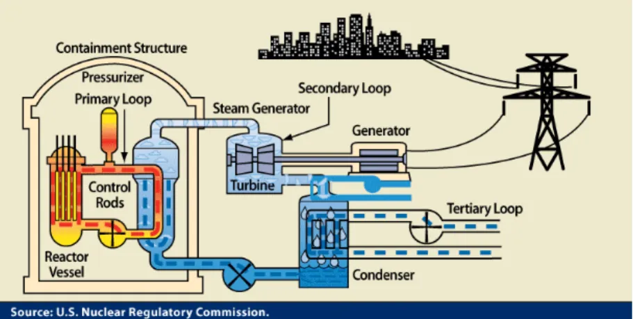
Similarly to a gas-fired station, a nuclear power plant generates electric-ity by converting thermal energy to mechanical energy, which is then con-verted to electricity [Reuss 2012]. In a nuclear reactor, the initial energy (heat source) comes from the fission of heavy nuclei into lighter nuclei in-side the reactor core. The heat is then passed (directly or not) to a work-ing fluid (water or gas), which runs through turbines. Figure I.1 illus-trates the functioning of a Pressurized Water Reactor (PWR). However the

Figure I.1: Conceptual scheme of a Pressurized Water Reactor (PRW). heavy nuclei used in a nuclear reactor, typically uranium 235_{U or}

pluto-nium239_{Pu, rarely undergo spontaneous fission (for instance the}235_{Uhas a}

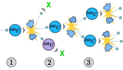
long half-life of 710 million years [Reuss 2012]). Fissions are in fact mainly induced by neutrons that collide with the nuclei constituting the surround-ing medium (fuel). Then, conveniently, the fission of these heavy nuclei produce new neutrons that can thus also collide with other nuclei and start a nuclear chain reaction (see Fig. I.2). This type of medium that supports the multiplication of neutrons is called a multiplying medium or fissile material. For instance, the induced fission of the235_{Ugives rise to two lighter nuclei,}

called fission products, and to a certain number of new neutrons n. A typical induced fission reaction is [Reuss 2012]:

n+235U!92 Kr+141Ba+3 n , (I.1) which liberates an energy of ⇠ 200 MeV1_{. The neutrons released by this}

reaction are emitted with a high mean energy of approximately 2 MeV. In a PWR, the chain reaction in fact requires neutrons to be slowed down to a thermal energy of the order of ⇠ meV (slow neutrons) in order to induce a fission (in heavy water, the thermal energy of neutrons is ⇠ 25 meV [Bussac

and Reuss 1978]); this is not true for a fast neutron nuclear reactor.

I.1.1 Neutron as a Point Particle

The aim of neutron transport theory is to describe the behaviour of the neutron population inside a nuclear reactor. For this purpose, neutrons are considered as point particles evolving within the reactor, where they interact only with the nuclei of the medium. This representation, which could seem too simplified, proves to be appropriate most of the time. In this section we briefly discuss its validity; then, we will assume that this representation holds in the rest of the thesis.

a. No relativistic effects

Neutron energy in a nuclear reactor typically goes up to 20 MeV (see Fig. I.5), i.e. a classical speed

v = r

2E

m ' 1.38 ⇥ 10

4p_{E(eV) m/s , (I.2)}

of the order of ⇠ 107 _{m/s, where m ' 939.565378 MeV/c}2 _{is the rest mass}

of the neutron. Indeed, the mean velocity of fast neutrons (released from fission) is more precisely 1.9 ⇥ 107 _{m/s. This order of magnitude of the}

speed of the fastest neutrons is small enough, compared to the light speed c ⇠ 3 ⇥ 108m/s, to consider that relativistic effects can be reasonably ne-glected [Schwarz and Schwarz 2004].

1_{This is a huge amount of energy (compare to the amount produce by a gas-fired power}

station):1 g of235_{Ucould potentially provide 2 ⇥ 10}4_{kWh of power, enough to run a 100 W}

1

Figure I.2: Scheme of a fission chain reaction, adapted from wikipedia. 1) An first neutron, leaving from a source, is absorbed by a nucleus of Uranium-235, causing its fission into two lighter nuclei and 3 neutrons (second generation of neutrons) accord-ing to reaction Eq.(I.1). This fission also releases/liberates a binding energy of ⇠ 200 MeV.

2) Among the 3 neutrons, two are lost for the chain reaction: one is absorbed by a238_{Uthat does not undergo a fission, the}

other for instance leave the system (absorbed by its bound-aries). The last neutron collides with an other 235_{U, which}

then divides/splits into two lighter nuclei and gives rise to a third generation of neutrons, with 2 neutrons.

3) Each of these 2 neutrons undergoes a collision with a235_U

causing their fission into lighter nuclei and a fourth genera-tion of neutrons.

The chain reaction is thus maintained until there is not enough heavy nuclei (aging of a reactor) or no neutron any-more (stopping of a reactor) in the system.

b. No interference: particle description

In transport theory, neutrons are considered as particles that can be fully described by their position and their velocity [Bell and Glasstone 1970]. In fact, quantum effects affecting the neutron transport, such as diffraction or interferences, can be neglected if the characteristic length of the medium (inter-nucleus distance ⇠1Å) is significantly larger than the neutron wave length. De Broglie’s wavelength of a neutron [De Broglie 1924], B, is given

by the relation: B= h p ' 2.86 ⇥ 10-11 p E(eV) m , (I.3)

where h ' 4.1343359 ⇥ 10-15_{eV·s is the Planck constant and p denotes the}

momentum of the neutron considered,

p=p2mE , (I.4)

for a non relativistic particle. m ' 939.565378 MeV/c2 _{is the rest mass of}

the neutron and E its energy. In a nuclear reactor, fast neutrons emitted from a fission have an energy of several MeV, for which B ⇠ 10-14m, i.e.

sev-eral orders of magnitude smaller than the characteristic distance between nuclei ⇠ 10-10_m.

Moreover, Heisenberg’s uncertainty principle [Heisenberg 1930] states a condition on the precision that can be accessed for the position and the momentum of a particle, formulated by [Kennard 1927]:

x p> h

2 , (I.5)

where x and p are respectively the standard deviation of the position and the momentum of the particle, and h = h/(2⇡) is the reduced Planck constant. Inside a reactor core (in most materials), neutrons have a mean free path (between two collisions with nuclei) of the order of a centime-ter [Reuss 2012]. For this reason, we could considered for instance that an uncertainty of 10-4 _{cm on the position of a neutron can be tolerated.}

Thus, using Eq. (I.4) in the relation Eq. (I.5), we find that the minimum uncertainty accessible on the energy E of the particle would be [Bell and

Glasstone 1970]

E(eV) ⇠ 10-5pE(eV) , (I.6)

which is negligible compare to the energy E itself. The position and the energy (or speed) of a neutron in neutron transport theory can thus be con-sidered with a good precision without violating Heisenberg’s uncertainty

principle. As a consequence, it is reasonable to consider neutrons as parti-cles (as opposed to waves) that can be characterised by their position and velocity.

Interference effects can be relevant for a tiny fraction of neutrons with very low energy (down to several meV). The wave length becomes in this case very large ( B⇠10-10- 10-9m) and neutrons can not be localized.

Be-cause of the negligible number of neutrons concerned, this effect is usually reasonably neglected in neutron transport theory [Bell and Glasstone 1970]. Note that in reactor physics, distances are often measured in centime-ters, as a reference to the centimeter mean free path of neutrons [Reuss

2012].

c. Neutrons interact only with the nuclei of the medium

Neutron-neutron interactions are neglected [Rozon 1998]. Indeed the prob-ability of such an interaction is negligible compared to the probprob-ability of a neutron-nucleus interaction, due to the huge difference in density: even in a thermal reactor, operating at high neutron flux, the neutron density is still less than 1011 _{neutrons per cm}3_{, whereas the nuclei density is of the order}

of 1022_{nuclei per cm}3_{[Bell and Glasstone 1970].}

As a consequence of paragraph b. and c., the spatial extension of neu-trons is not relevant for the problem of their transport through matter. For these reasons, they can be considered as point particles (i.e. 0-dimensional particles), and the neutron population can be thought of as an ideal gas (de-fined as a gas of particles that do not interact which each other).

d. Neutron radioactive instability is neglected

Outside a nucleus, a free neutron is unstable and can decay into a proton (beta decay):

n ! p++ e-+ ¯⌫e,

where p+_{, e}-_{and ¯⌫}

e respectively denotes the proton, the electron and the

electron antineutrino. Within this decay, neutrons have a life time of about 15 min [Yue et al. 2013]2_{, which is very large compared to the millisecond}

characteristic life time of a neutron within a nuclear reactor [Bussac and

Reuss 1978]. The probability that a free neutron actually undergoes a beta

decay in a nuclear reactor before encountering a nucleus is thus very small and this effect is as a consequence neglected.

2_{more precisely, a life time of 887.7 ± 1.2[stat]±1.9[syst] s was recently measured by [Yue}

e. Other hypotheses

Very frequently, two other hypotheses are made in neutron transport the-ory: that the fluctuations of the neutron population can be neglected [Bell

and Glasstone 1970], and that the displacements performed by neutrons

inside a nuclear reactor belong to a class of processes called exponential dis-placements (described in the next section). The discussion of these two last hypotheses will be at the heart of this thesis.

I.1.2 From Neutron Transport in Multiplying Media to Branching Exponential Flights

In this section, we recall the processes that govern neutron transport in (lo-cally homogeneous) multiplying media. We will see that this transport can be described in terms of a specific type of random walks, called branching exponential flights.

a. Transport - Exponential Random Walks

Consider a single neutron3 _{flowing through and interacting with a}

back-ground material. Based on the previous considerations, this neutron under-goes a sequence of displacements, separated by collisions with the nuclei of the surrounding medium. We also assume that, between two collisions, no forces act upon the particle, such that its momentum is preserved along each of its displacements (free displacements): between collisions, the neu-tron therefore travels in a straight line and with a constant speed [

Pomran-ing 1991]. Consider now that the neutron leaves a collision at a time t0from

a position r0with a speed v0in a direction !0: its path from r0to the next

collision then follows the trajectory 8 > < > : r0 _{= r0+ s}0_{!0 ,} t0 = t0+ s 0 v0 . (I.7)

The curvilinear coordinate s0_{parametrises the rectilinear trajectory, varying}

from 0 at the initial point r0, to s at the next collision (s thus corresponds

to the distance travelled between the two collisions). Due to the quantum nature of the neutron-nucleus interaction and to the huge number of nu-clei inside the reactor core, the exact position r of this collision can not be assessed deterministically. In fact, as the neutron travels through the fissile

3_{Even though our work mostly focuses on neutron transport, most of the results}

pre-sented throughout the thesis also apply, with minor modifications, to other “neutral parti-cles”, i.e. particles which do not interact with matter until they undergo a collision with the traversed medium, such as photons in the classical limit [Kalos and Whitlock 2008].

material it has, at anytime, a certain probability to interact with a nucleus that depends only on the local properties of the surrounding medium. It is thus reasonable to assume that a neutron evolves in the medium with no memory of its past history [Pomraning 1991]. This property of the neu-tron transport is said Markovian4_{. As a consequence, the probability that}

a neutron interacts with the surrounding medium while travelling a small distance ds0_{about s}0_{is proportional to the distance travelled ds}0_(and

inde-pendent on the length already travelled) and given by

Probability of interaction ⌃(r0, v0)ds0. (I.8)

The proportionality constant ⌃ depends only on the local properties of the medium in the phase space position5 _(r0_{, v0). The dependence in the}

di-rection of travel !0 of the particle is omitted, as the medium is generally

assumed to be isotropic. In transport theory, the quantity ⌃ is called [

Pom-raning 1991]

Total cross section (cm-1_{) ⌃(r, v}

0); (I.9)

it is the probability of interaction per unit length. Note that this cross sec-tion is a macroscopic cross secsec-tion6_{. As a result of Eq. (I.8), the distance s}

travelled by a neutron between two collisions, along the trajectory Eq. (I.7), is given by the probability density function (pdf) T(s) [Kalos and Whitlock

2008;Hughes 1996;Weiss 2005]: T(s) = ⌃(s) exp  -Zs 0 ⌃(s 0_)ds0 _{for s > 0 . (I.10)}

In this equation, the parameter s0 _{contains the information about the}

local position r0_(s0_{)of the particle, given by Eq. (I.7).}

Intercollision distances for a non-homogeneous Poisson process

Here, scattering centres encountered by neutrons along their trajectory are

4_{In a Monte Carlo simulation for example this property implies that the neutron can}

be stopped at any moment and then restarted without taking into account what happened before it was stopped: the knowledge of the current phase-space position of the walker (r, v) is sufficient to determine its future evolution. Note that the knowledge of the current

position only is not sufficient to ensure the Markovianity, as it would be instead the case for a Brownian particle [Chung 2013].

5_{We consider that the density of nuclei (scattering centres) is high enough that the}

mul-tiplying medium can be described as a continuous medium, characterised by cross-section that is homogeneous at the scale of a volume element dr (locally homogeneous).

6_{Various types of collisions can happen in the medium. The macroscopic cross section}

for a collision type i, ⌃i(r, v0), is given by the density of nuclei in the vicinity of r multiplied

by the microscopic cross section of the nuclei i(v0)(cm2or barns) for this type of collisions:

⌃i(r, v0) = n(r) i(v0)[Reuss 2012]. The total macroscopic total cross section is then ⌃t=

P

non necessarily uniformly distributed, and the process performed by neu-trons while travelling (jumps separated by collisions given by ⌃(s)) is called non-homogeneous Poisson process7 _{[Ross 2013]. In Eq. (I.10), the second}

fac-tor, exp⇥-Rs₀⌃(s0)ds0⇤, is the marginal probability that the path gets as far as s (without collisions in the meanwhile), whereas the first factor ⌃(s) cor-responds to the conditional probability, ⌃(s)ds, that the collision occurs in ds about s. In analogy with optics, the exponentRs

0⌃(s0)ds0is often called

optical path length [Bell and Glasstone 1970]. In homogeneous media, for which the cross-section ⌃ is constant, this exponent reduces to s ⌃, and the jumps pdf becomes independent of the local position of the particle, taking simply the exponential form:

Exponential Distribution T(s) = ⌃ exp [-⌃ s] . (I.11)

Intercollision distances for a homogeneous Poisson process

In this case, the scattering centres encountered by the neutrons are uni-formly distributed in space (⌃ = cst), and the collision process followed by neutrons is called homogeneous Poisson process.

Proof

To demonstrate Eq. (I.10), we refer toKalos and Whitlock’s book

on Monte Carlo methods[2008, sec. 6.3]. By definition the pdf T

must be normalised on positive values, and can thus be associ-ated to a

cumulative distribution Zs

0 T(s

0_)ds0 _{=1 - U(s) . (I.12)}

Its complement U(s) =R_s+1T(s0)ds0is the marginal probability that the next collision is at a distance s0 _{larger than s. It can be}

decomposed into the sum of two probabilities:

U(s) = U(s +ds) + P(s6 s0 < s+ds), for ds > 0 , (I.13) the probability that the collision occurs after s + ds, and the prob-ability P(s 6 s0 _{< s+ds) that it occurs between s and s + ds.}

This latter probability can be rewritten using Bayes’ formulaa_for

conditional probabilities:

P(s6 s0< s+ds) = U(s) P(s6 s0< s+ds | s0 > s) . (I.14)

7_{Along the trajectory, the number of nuclei distributed along the interval (s, s + s} 1)is

a random variable that follows a Poisson law ([Poisson and Schnuse 1841]) with a mean Rs+s1

This latter conditional probability is the probability that a colli-sion occurs between s and s + ds for a process starting from s; for small ds it can thus be easily expanded using equation (I.8): P(s 6 s0 < s+ds | s0 > s) = ⌃(s) ds + o(ds). Replacing these results in equation (I.13) in the limit where ds goes to 0 leads to a first order differential equation verified by U:

-U0(s) = U(s) ⌃(s) + o(1) , (I.15) whose solution is:

U(s) =exp  -Zs 0 ⌃(s 0_)ds0 _{, (I.16)}

knowing that U(0) = R+1

0 T(s)ds = 1 by normalisation of the

pdf T. The result Eq. (I.10) then stems from the definition of the complementary cumulative: T(s) = -U0_(s).

a_{Bayes’ formula for two propositions A and B: P(A | B) =}P(A\ B)

P(B)

Note that the jump pdf Eq. (I.10) commonly takes an other form, where the current position and speed of the particle are clearly specified [Spanier and

Gelbard 1969;Lux and Koblinger 1991]:

T(s|r, !₀, v₀) = ⌃(r, v₀)exp  -Zs 0 ⌃(r - s 0_! 0, v0)ds0 , (I.17)

Intercollision Length Probability Density Function

is the pdf of the jump length s performed by a particle arriving at a collision in r with a velocity v0!0(see Eq. (I.7)). This expression of the jump pdf is

widely used in reactor physics. Observe that this pdf is not a density of the three space dimensions, but only of one, corresponding to the travelled length s. In the same way, we can also rewrite the marginal probability Eq. (I.16), U(s|r, !0, v0) =exp  -Zs 0 ⌃(r - s 0_{!0, v0)ds}0 _{, (I.18)}

being the probability that a particle arriving in r has travelled a distance s with a constant velocity v0!0without encountering any collision.

Following this process of random jumps separated by collisions, the path performed by a neutron is thus random, called random walk, or, more precisely, exponential walk in the case of an homogeneous medium. For nu-merical simulation purposes, the sampling of a random variable from an

Figure I.3: Schematic representation of one initial neutron and its descendants. Neutron-nucleus interactions are commonly grouped in three main types: scattering (blue dots), fis-sion (green circles), and sterile capture (black stars). These events confer a branching structure to the neutron path. exponential distribution Eq. (I.11) is illustrated in appendix 4. b. Collision - Branching process

Neutron-nucleus interactions are very complex, in that they are governed by quantum physics and involve the strong nuclear interaction. However, they can be conceptually grouped in three main types [Reuss 2012]: sterile capture, scattering or fission (see Fig. I.3). In the following, each of these events will be briefly recalled, and their physical meaning will be related to the corresponding statistical physics interpretation. In doing so, we will introduce the notation commonly used in reactor physics.

Capture events occur with a probability pc(r, v) for particles arriving at

a collision about r with a speed v: the incoming particle disappears, ab-sorbed by a nucleus, and its branch of the walk ends (see Fig. I.4). In reactor physics, this event corresponds to a sterile capture (absorption that does not cause fission) and is associated with the macroscopic capture cross section: capture cross section ⌃c(r, v) = pc(r, v) ⌃(r, v) . (I.19)

where ⌃(r, v) is the total cross section defined in Eq. (I.9). According to its definition above, ⌃c(r, v) is the rate at which absorption events occur. As

for the total cross section, this quantity is known to depend on the position r and the speed v of the considered particle.

Figure I.4: Neutron-nucleus interactions can be conceptually grouped in three main types:

- Sterile capture: the incoming neutron is absorbed;

- Scattering: the speed and the direction of the neutron change, from v0!0 to v1!1;

- Fission: the incoming neutron is absorbed, k new neutrons are emitted with new speeds v1..k and directions !1..k.

Scattering events occur with a probability ps(r, v), whereupon the

veloc-ity (direction and speed) of the walker is redistributed at random, following the probability density function Cs(v ! v0|r) (see Fig. I.4), calledscattering

kernel. This scattering kernel is in general speed dependent and anisotropic (more precisely it depends on the angle ✓ between the incoming and the outgoing directions: ! · !0 _{= cos(✓)). This type of event is related to the}

macroscopic

scattering cross section ⌃s(r, v) = ps(r, v) ⌃(r, v) . (I.20)

Fission events give rise to two different types of neutrons, theprompt neu-trons, emitted instantaneously8_{after the fission event, and the delayed}

neu-trons, emitted from a few milliseconds to a few minutes later. As prompt neutrons represent more than 99% of the emitted neutrons, we will first fo-cus on them, without taking into account delayed neutrons. We will then see in Sec. I.2.2 how the existence of delayed neutrons modifies the dy-namics of the neutron population. At a collision, a fertile capture (fission, see Fig. I.4) occurs with a probability pf(r, v): the incoming neutron is

ab-sorbed and k new neutrons are emitted with respective probabilities pk

in a new direction !0_{with a new velocity v}0_{given by the probability density}

Cf(v ! v0|r). Generally, new directions !0are isotropically distributed and

the pdf Cf(v ! v0|r) depends only weakly on the incoming velocity v:

Cf(v ! v0|r) =

1

4 ⇡Fp(v0), (I.21)

where Fp(v0)is the speed spectrum of prompt fission neutrons, called average

Average Prompt Fission Neutron Spectrum

The kinetic energy of an outcoming fission neutron is distributed over several decades, from fractions of meV to about 10 MeV. In 1960, Terrell [1957] proposes two approaches to model the prompt fission neutron spectrum: the Maxwellian and the Watt-Cranberg spectrum representations. Most modern assessments of prompt fission neutrons rely on a model developed by

Mad-land and Nix[1982] in the 80s.

0 0.1 0.2 0.3 0.35 0 4 8 12 E (MeV)

Figure I.5: Maxwell (in red) and Watt (dash curve) spectrum for Uranium. Parameters are optimally adjusted to the experimental spectrum for each fissioning system at a given excitation energy [Antoni and

Bourgois 2013]. For Uranium, the mean energy

of a prompt neutron is about 2 MeV.

prompt fission neutron spectrum (see Fig. I.5). The normalisation factor 4 ⇡ = ⌦3is the maximum solid angle in a 3-dimensional space:

⌦3 =

ZZ

Sp3

d2! =4 ⇡ , (I.22)

which corresponds to the surface of the 3-dimensional unit sphere Sp3.

d2_{!/(4⇡) is the probability for a neutron to be emitted in the solid angle}

element d2_{!about the direction ! (isotropic distribution of the outgoing}

directions). By definition, the probability family {pk}k>0 verifies the

nor-malisation

X

k>0

pk = 1 . (I.23)

In principle the number k of emitted neutrons after a fission could vary from 0 to +1, but in practice k only varies from 0 to 7 [Reuss 2012]. The

mean number of neutrons produced per fission, ⌫=X

k>0

k pk , (I.24)

is a relevant parameter to characterise the production of neutrons. The occurrence of fission events is defined in terms of the macroscopic

fission cross section ⌃f(r, v) = pf(r, v) ⌃(r, v) . (I.25)

The three events The probability of occurrence of each of these three

events is normalised, pc+ ps+ pf = 1, so that the cross sections similarly

add up to

⌃(r, v) = ⌃c(r, v) + ⌃s(r, v) + ⌃f(r, v) , (I.26)

where the three types of event composing the total cross section appear clearly.

Therefore, submitted to these three types of collisions, each neutron of the population can, at any moment, die by absorption or give birth to other neutrons by fission. Each neutron has thus descendants (except for the ones that die) and an ancestry (except for the ones emitted from a source). In this sense, the dynamics of reproduction and death of neutrons in the popula-tion is similar to the one of families, which was first studied by Bienaymé (1845) [Heyde and Seneta 1977] and by Galton and Watson [Watson and

Galton 1875] on their investigation of the extinction of family names. The

process of reproduction and death is known as Galton-Watson process or branching process [Harris 1963], in reference to the branching structure that it confers to the family (like a family tree - see Fig. I.3). Depending on the value of ⌫, defined in Eq. (I.24), the process is then said to be [Harris 1963]:

subcritical ⌫ <1 ;

critical ⌫=1 ; (I.27)

or supercritical ⌫ >1 .

Note that, in reactor physics, the dynamics of a neutron family can thus be followed in time, but also in generation (see Fig. I.2): neutrons leaving from a source are considered as the first generation of neutrons; then at each event (scattering or fission) a neutron leaving a collision belongs to the generation after that of the one entering the collision.

Monte Carlo Numerical Simulations for Neutron Transport

The different processes we have seen in this section are at the basis of Monte Carlo simulations developed for the transport of neutrons in a multiplying medium [Spanier and Gelbard 2008]. Indeed this type of simulation involves following the trajectory of each particle within the medium from its source to the end of its history (by absorption or exit of the medium) [CEA

monogra-phie 2013]. Along this trajectory, one or several physical

observ-ables (random variobserv-ables) are recorded, such as the total length travelled inside a certain region of the medium, or the total num-ber of collisions performed in this region. Simulations of the full history of the system are performed a large number of times, in order to obtain the mean of each observable over the various realisations of the system. These averaged values are called es-timators, and will be seen more in detail in Chapter 2. Monte Carlo methods are not limited to neutron transport, and have many applications involving stochastic processes in physics, life sciences and finance [Gobet 2013;Krauth 2006].

c. Generalised process and unified notation for branching random walk

The mechanisms governing neutron behaviour in multiplying media confer a random branching structure to the neutron paths, with random displace-ments, death and reproduction events. Neutrons inside the reactor core thus perform random walks with a branching structure, known as branch-ing random walk in statistical physics9_{. Besides, since the length of the}

dis-placements are exponentially distributed (if the medium is homogeneous), such random walks are called branching exponential walks.

However, the complexity of the reactor physics formalism and notation, with different type of collisions (various cross sections ⌃c/s/fand

proba-bility density functions Cc/s/f), may hinder the statistical analysis of some

of the key physical mechanisms of the neutron transport. For the sake of simplicity, we consider the general branching random walk process with only one type of collision (see Fig. I.6), upon which the incoming particle disappears, and k new particles are emitted with a probability pk(r, v). The

velocities v0 _{of the new particles are then redistributed, following a single}

probability density function C(v ! v0_{|r). Each descendant will then behave}

as the mother particle, undergoing a new sequence of displacements and collisions, giving thus rise to a branched structure. It is finally possible, for

9_{In particular, when p}

k= k,1(i.e. without branching), the walk described in the current

section, with random jumps separated by random reorientation of the walker, is known as Pearson random walk [Hughes 1996;Weiss 2005].

Figure I.6: Conceptual representation of the three groups of collisions in nuclear reactor physics with its specific notation, and of the generalised branching process with a unified notation. practical applications, to replace the general notation by the one specific to reactor physics, using the transformation (see Fig. I.6):

⌫ ⌃(r, v) C(v ! v0|r)

# (I.28)

⌃s(r, v) Cs(v ! v0|r) + ⌫ ⌃f(r, v) Cf(v ! v0|r)

From unified notation to reactor physics notation

Results specific to nuclear reactor physics will then be identified by a yel-low bar on the left margin of the text, as it is on Eq. (I.28).

I.1.3 Characterisation of the neutron population: phase space densities

Neutron transport in nuclear reactors is intrinsically stochastic, due to the random nature of the different physical phenomena (random collisions and changes of velocity) that govern the neutron behaviour. As a consequence neutron transport problem must be handled within the framework of a

sta-tistical description. In order to fully characterise the neutron dynamics in the phase space, each neutron requires six variables at any time t or current generation i of the particle:

– the three spatial coordinates r;

– the three velocity coordinates v, which contain information about the speed v (or any related variable such as the kinetic energy E) and the direction ! of the particle.

Although the neutron population is very diluted compared to the popu-lation of nuclei, it is still very large ⇠ 108 _neutrons/cm3 _{in a power}

reac-tor [Duderstadt and Hamilton 1976]. As consequence, the statistical analy-sis of all the individual positions can be, most the time, replaced by a mean analysis using the concept of expected densities10 _{in the phase space [}

Dud-erstadt and Hamilton 1976]. For this purpose, we replace the microscopic

description of each neutron by a description at a mesoscopic scale, assum-ing that the neutron density is locally homogeneous: homogeneous over any volume element d⌧ = dr dv of the phase space.

We are thus interested in densities in the phase space: spatial and angu-lar densities with respect to the six variables, r, v. The dependence on time or generation will be denoted with a small index, or a seventh variable, t or i, which will stand for distinguishing out of equilibrium cases from sta-tionary cases.

Speed and Kinetic Energy

In transport theory it is convenient to use the kinetic energy E and the direction ! of the particle, rather than the three momen-tum or velocity variables v = v !, for easier reference and com-parison with experimental data [Pomraning 1991]. In the follow-ing, however, we will keep the notation with the velocity for the sake of simplicity. Note that these two notations are perfectly equivalent, as E and v are related by the classical mechanics re-lation E = m v2_{/2. Thus, any density function p can be written}

in term of the variable v or E, using the identity:

p(v)dv = p(E)dE , (I.29)

where the relation between dv and dE is then given by

dE = m v dv or dv = dE/p2 m E . (I.30)

a. Particle Density (⇠ 108 _n.cm-3 _{in a power reactor) [Duderstadt and Hamilton}

1976]

For instance, let us first start with a central quantity, the

Particle angular density (n.cm-3.sr-1.MeV-1) n(r, v, t) . (I.31) As a density in the phase space, n(r, v, !, t) d3_{r dv d}2_{! corresponds, at a}

certain time t, to the mean number of particles – located in a small volume d3_{r about r,}

– whose speed is between v and v + dv,

– and which travel in a direction given by the solid angle d2_{! about}

![Bell and Glasstone 1970].

The integration of this particle angular density over all possible directions, leads to the particle density (n.cm-3_.MeV-1_):

particle density n(r, v, t) = ZZ

⌦3

d2_{! n(r, !, v, t) . (I.32)}

This quantity gives the distribution in space and energy (speed) of neutrons in the system at any time. The ensemble of the possible directions is given by the solid angle ⌦3 = 4⇡ defined in Eq. (I.22). The neutron density

cap-tures most of the information needed to describe the statistical behaviour of the neutron population inside nuclear reactors. In fact, this quantity lies at the heart of two other physical observables that are more commonly used in reactor physics: the neutron flux and the reaction rate [Bell and Glasstone

1970].

b. Collision Rate Density, or Reaction Rate Density

The neutron density allows us to compute the rate at which neutron-matter interactions occur at any position in the reactor [Reuss 2012;Bell and

Glas-stone 1970]. Between two collisions, a neutron keeps a constant velocity

v !. During a time interval dt, it thus travels a straight path of length v dt, and therefore has the probability ⌃(r, v) v dt to interact with the surround-ing medium about r. Multiplysurround-ing this probability by n(r, v, t) d3_{r d}3_{v (the}

mean number of neutrons in the vicinity of r with a velocity v) leads to the mean number of collisions that occur during dt in the volume element d3_{r d}3_{v of the phase space, and thus to define the}

Collision rate angular density (r, !, v, t) .= n(r, !, v, t) ⌃(r, v) v , (I.33) (collisions cm-3_.MeV-1_.sr-1_.s-1_{). In other terms, (r, v, !, t) d}3_{r d}3_{v is the}