COMSOL Finite-Element Analysis: Residual
Stress Measurement of Representative
304L/308L Weld in Spent Fuel Storage
Containers
by Dominic Solis
Submitted to
Department of Nuclear Science and Engineering in Partial Fulfillment of the Requirements for the Degree of
Bachelor of Science in Nuclear Science and Engineering at the
Massachusetts Institute of Technology
June 2014
@
2014 Dominic Solis. All rights reserved.The author hereby grants to MIT permission to reproduce and to distribute publicly paper and electronic copies of this thesis document in whole or in part in any medium now
known or hereafter created.
Signature of Author ...
Signature redacted
Department of Nuclear Science and Engineering May 9, 2014
Certified by
Signature redacted
Ronald Ballinger rofe sor of Nue ar Scie e and Eng. a rial S i nce and Eng.
-/1/s
Sn ervisorAccepted by
....
Signature redacted...
(
Richard K. LesterProfessor and Head of the Department of NSE
MASSACHUSETTS INSTITI ITE OF TECHNOLOLGY
JUN 02 2015
COMSOL Finite-Element Analysis: Residual
Stress Measurement of Representative
304L/308L Weld in Spent Fuel Storage
Containers
by Dominic Solis
Submitted to Department of Nuclear Science and Engineering on May 9th, 2014 in Partial Fulfillment of the Requirements for the Degree of
Bachelor of Science in Nuclear Science and Engineering
Abstract
The ultimate storage destination for spent nuclear fuel in the United States is currently undecided. Spent fuel will be stored indefinitely in dry cask storage systems typically located on-site at the reactor or at a dedicated independent spent fuel storage installation (ISFSI). Since these canisters were not originally designed or qualified for indefinite storage, there is a need to quantify the length of time they will be viable for storing spent fuel. Stress corrosion cracking (SCC) is a concern in these canisters if they are exposed to an aqueous, chloride-containing film. Canisters are fabricated using a concrete overpacking, along with austenitic stainless steel on the inside which is welded together. One factor that would significantly impact SCC behavior inside these canister welds, if the proper conditions developed such that SCC occurred, is the tensile residual stress profile. As the highest residual stresses are present in the welds and their heat-affected zones (HAZ), it would be useful to investigate their influence by predicting the residual stress profile in the container. These data will support further research into the life expectancy of these canisters and the possible ways in which they might fail due to SCC. Residual stress data for nuclear waste canisters are scarce. Without experimental measurements, initial insight must be attained through computational analysis using finite-element analysis (FEA) packages such as COMSOL.
Using a representative 304L/308L weld plate as a model in COMSOL, predicted residual stress shows some agreement with expected trends: high tensile stresses in the weld/ HAZ regions and compressive stresses in the surrounding material. Hardness tests show trends similar to the hardening profiles that were created after the weld simulation. Additionally, the thermal model may offer insight in predicting the HAZ profiles in the weld. While the 2D model is simplified and would benefit from further refinement and validation, preliminary results suggest that FEA could be used for residual stress measurement predictions.
Thesis Supervisor: Ronald Ballinger
Acknowledgements
I would like to thank Professor Ballinger for suggesting this investigation, as well as the support given for this research. This project could not be accomplished without the resources at the H. H. Uhlig Corrosion Lab.
I am grateful to graduate student, Sara Ferry, for being the gateway to join the overall
project and sharing her insight in lab. Along with undergraduate Isabel Crystal, the research process was made enjoyable with the tireless work done on hardness testing, sensitization experiments, and data library mining. Additionally, I'd like to thank Assistant Professor Mike Short for introducing me to Lyx, as formatting papers, such as this thesis, have been quite easy ever since.
An indescribable amount of thanks and love go out to my parents, Eric and Clarissa Solis, who have supported me to get to where I am now ever since I can remember. Addi-tionally, I am extremely grateful to my extended family for being instrumental for making my education experience possible.
To everyone met along this culmination, thank you for pushing me in every intentional and unintentional way.
Contents
1 Introduction 9
1.1 SCC in Nuclear Spent Fuel Storage Containers . . . . 9
1.2 The importance of residual stresses and measurement . . . . 10
2 Background 10 2.1 Residual Stress . . . .. . . . . 10 2.2 Experimental Measurement . . . . 11 2.2.1 Neutron Diffraction . . . . 11 2.2.2 Contour Method . . . . 12 2.3 Computational Measurement . . . . 13
2.3.1 COMSOL Multi-physics Finite Element Analysis (FEA) . . . . 13
2.4 Governing FEA Equations . . . . 14
2.4.1 Stress-Strain Relationship & Isotropic Hardening . . . . 14
2.5 Vicker's Hardness Test . . . 15
3 Methodology 16 3.1 304L/308L Weld Sample . . . . 16
3.2 Characterization . . . . 16
3.2.1 Metallography . . . . 17
3.2.2 Vicker's Hardness Testing . . . . 18
3.3 Geometry & Meshing. . . . 19
3.4 Material Properties. . . . . 21
3.5 Thermal Model . . . 21
3.6 Boundary Conditions. . . . . 22
3.7 Time-stepping Settings. . . . 22
4 Results 23 4.1 Hardness Testing Results . . . 23
4.2 Residual Stresses . . . 25 4.3 Temperature Profiles . . . 26 4.4 HAZ Predictions . . . 27 5 Discussion 28 5.1 Hardness Testing . . . 28 5.2 FEAValidation. . . . 28 5.3 Study Extensions . . . 29 6 Conclusions 29 7 Appendix 32
List of Figures
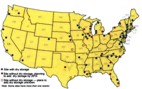
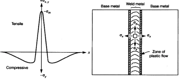
1 Spent Fuel Dry Storage Sites at U.S. Nuclear Reactor Power Plants (2010). [11] 9 2 Longitudinal and transverse stress distribution from a butt weld on a metal
plate. Tensile regions from where the weld material solidified, balanced by
surrounding compressive regions in the base metal.[2] . . . . 11
3 Neutron diffraction map of potential data points for a surface of a sample. As tensile stresses develop in the weld and HAZ regions, there is a concentration of points in these areas of interest. . . . . 12
4 Illustration of the superposition principle to calculate resulting residual stress with the contour method. [3] . . . . 13
5 When a load on a material increases the stress past yielding, there is a strain-hardening that increases the yield stress from uys,init to O-ys,new. After un-loading and the material is relaxed, a plastic strain can be defined as well as an elastic strain recovery. Adapted from [4]. . . . . 15
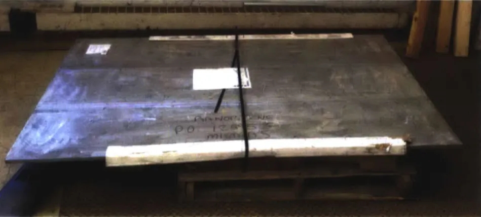
6 Full 6'x4' weld plate received from Ranor. . . . . 16
7 Sectioned piece of the weld received from Ranor Incorporated. . . . . 17
8 Weld sectioned sample after etching with Kalling's Reagent. The weld bead's shape can been seen with the added contrast. . . . . 17
9 50x micrograph showing Ranor sample microstructure near weld boundary and HAZ. A length unit of 500 microns is labeled near the fusion line. Larger grains are seen in the HAZ area just outside weld boundary. . . . . 18
10 Composite image of four micrographs from the weld edge and into the weld sam p le. . . . . 18
11 Map of Vicker's hardness test on the weld sample. The sample is about 68 mm across in width. L, R, and H denote left, right, and HAZ horizontal scans, respectively. . . . . 19
12 Micrograph near weld boundary. Measurements were digitally taken in order to plot where data points were taken. . . . . 19
13 Weld geometry, in mm, as defined in COMSOL anchored at the center of the material. The darker trapezoidal regions are the weld bead shapes used. The measurement ticks on the side show the width extending from 4 mm at the center to 20 mm at the top and bottom surfaces. The height is shown as 15.875 m m . . . . 20
14 Weld mesh as defined in COMSOL using quadratic elements. Fixed distribu-tions were set to increase the density of elements within the weld and near the weld boundary, while the density decreases in the outer regions to reduce com putation tim e. . . . . 20
15 Strain-hardening induced by the thermal process. The initial yield stress of both 304 and 308 stainless steels can be seen to increase around the weld regions when the welding is completed and cooled. . . . . 23
16 HV results for test points corresponding to (L) on the sample map. . . . . . 24
17 HV results for test points corresponding to (R) on the sample map. . . . . . 24
18 HV results for test points corresponding to (H) on the sample map. . . . . . 25
19 Longitudinal, transverse, and perpendicular components of residual stress. The longitudinal component is the most tensile at around 600 MPa, with the other components only reaching about 60 to 100 MPa. . . . . 25
20 Temperature profile of all 4 weld beads. Data is taken across the weld center-line at increasing distances away from the weld area. Therefore the first two weld beads, at the center, show elevated temperatures. Before each heat pass, the temperature is allowed to cool below 450 K, the approximate inter-pass temperature. .... . .. . ... ... .. ... . . .. .. . . .
21 Predicted HAZ regions, shaded in lighter color (orange), by combining the peak temperature contours at the respective weld bead time. The darker region (dark red) shows the areas that are melted. Based on a recrystallization
22 23 24 25 26 27 28 29
List
1 2temperature of 973 K and a melting temperature of 1683 is estimated to be about 3 mm from the fusion line. . .
Typical longitudinal stresses after welding. [5] . . . . Thermal conductivity of 304/308. . . . . Heat capacity at constant pressure of 304/308. . . . . .
Elastic modulus of 304/308. . . . . Poisson's ratio of 304/308. . . . . Density of 304/308. . . . . Surface emissivity of 304/308. . . . . Initial yield stress of 304/308. . . . .
f Tables
Compositions of the 304L base/ 308L weld materials.. Welding parameters used for the analysis. . . . .
26
K, the HAZ region
. . . 27 . . . 29 . . . . 32 . . . 33 . . . 33 . . . . 34 . . . . 34 . . . . 35 . . . . 35
3 Inter-pass and completion waiting periods for weld simulation. . . . .
16
22
27
1
Introduction
Dry casks for spent nuclear fuel were originally designed for temporary use. After a storage period of approximately 10 years, the used fuel would ultimately be transferred to a more permanent site such as Yucca Mountain. In 2010, the Presidential Administration's budget report called for the Yucca Mountain Nuclear Waste Repository Project to be terminated [6]. There is now a strong possibility that spent fuel will stay in these canisters for much longer than originally planned. Therefore, assessing the long-term life expectancy of these canisters will be an important investigation for the nuclear industry. Due to residual stresses left in the stainless steel welds after the fabrication of these canisters, a method of measurement is warranted to better understand their influence toward stress corrosion cracking (SCC).
1.1
SCC in Nuclear Spent Fuel Storage Containers
SCC is brittle failure (i.e. fracture) that occurs in a metal due to the combination of tensile
stresses and a corrosive environment [2]. In particular, SCC could occur in the stainless steel used in canister fabrication if an aqueous, chloride-containing environment is maintained on the canister surface. Deliquescence is the process by which salts, such as chlorides, can absorb moisture from the atmosphere and form a solution. As can be seen in Figure 1, some of these dry fuel storage sites are located near coastal regions, where atmospheric chlorides can attach to the exposed areas of the canister. Designs for dry cask storage systems usually consist of a welded austenitic stainless steel canister of types 304/304L or
316/316L, surrounded by concrete [7]. With the combination of the decay heat from the spent fuel and deliquesced corrosive solution, environmental conditions that allow for SCC can develop [8]. Together with the tensile residual stress present in the canister material, crack propagation becomes a possibility.
ORMI
JD W1,IY
WY
FsA Pa
NVddNEy
o
Figur 1: SpnNulDySoaeStsa ..NcerRatrPwrPat 21) 1
1.2
The importance of residual stresses and measurement
The most vulnerable section of the storage container is the sensitized heat-affected zone (HAZ) of the weld material [7]. When steel is welded and cooled, the material is subjected to large thermal gradients, and the resulting expansion and contraction leaves behind residual stresses. These residual stresses can be tensile, an important factor for SCC [9]. The residual stress profile of the canister steel will strongly influence this SCC behavior, and looking specifically at the weld and HAZ will be important. With regard to storage canisters in the United States, there are few measurements for the residual stress profile found in literature. Therefore, the overall study will lay important groundwork for future investigations involving a canister's residual stress profile for SCC.
Experimental and computational measurement methods have been developed for looking at these stresses. In particular, this investigation aims at using COMSOL, a finite-element software package, to identify the residual stress profile in a representative canister weld plate. In the future of the overall project, experimental measurements have been planned using neutron diffraction and the contour method for comparison.
2
Background
Residual stresses are stresses which are held in place within a material, without the presence of an external force acting on them [10]. These stresses can exist at different levels of depth within the microstructure of material, though not all are taken into account with current measurement techniques. Several experimental methods have been developed to measure residual stresses, but in addition, computational analysis with finite-element software is also used to investigate the phenomenon. In finite-element analysis (FEA), constitutive relationships are required to relate the welding simulation to residual stress formation. After the weld process, a hardening and softening of material occurs around the weld regions. For weld characterization, Vicker's hardness tests can be used to map the hardening differences that occur.
2.1
Residual Stress
Nearly all manufacturing processes on a material will create residual stresses, developing from an elastic response from local strains that can be due to non-uniform plastic defor-mation, surface modifications, or material phase/density changes. Three types of residual stresses exist in a material and can be defined as follows [101:
* Type 1 -Macro residual stresses that equilibrate across the whole body of the material * Type 2 -Micro residual stresses that exist on the order of microns between each other
in the microstructure and equilibrate across several grain boundaries
9 Type 3 - Atomic residual stresses that exist on the order of the material's crystal lattice structure and equilibrate across an area of a grain
Welding is an example of a manufacturing process that will introduce these local strains within a metal. During the welding process, the thermal transformation of the lattice structure introduces stress in the material. The weld metal is stress-free while molten, but as solidification occurs, large longitudinal tensile residual stresses are created in the weld metal and HAZ. These tensile regions must be balanced by compressive stresses in the
surrounding material [10]. The phenomenon is illustrated in Figure 2. These stresses can influence important material vulnerabilities, such as SCC, when the welded component is in service [2]. + X, y Tensile Compressive x -aI Weld metal
Base metal Wd Base metal
Zone of
plastic flow
Figure 2: Longitudinal and transverse stress distribution from a butt weld on a metal plate. Tensile regions from where the weld material solidified, balanced by surrounding compressive regions in the base metal.[2]
2.2
Experimental Measurement
As residual stresses are known to be present within a welded material, experimental methods are used for measuring residual stress. Current techniques look primarily at Type 1 residual stresses [10]. Examples of experimental methods include neutron diffraction and the contour method. These methods offer diversity in how stress is calculated, as well as how the sample physically needs to be prepared. In particular, the future project plans include using both methods to determine the residual stress influence on SCC and to validate the predicted results from the computational analysis.
2.2.1 Neutron Diffraction
As a non-destructive method, neutron diffraction can be a useful tool for investigating residual stress. The drawback of the technique is the required access to a source of neutrons, such as a nuclear reactor, to perform such an experiment. The principle of the method is based on the material being irradiated with neutron beam of wavelength A, comparable with the inter-planar spacing dhkI. With the resulting diffraction pattern, the lattice spacing can be determined through Bragg's law, shown in Eq. 1 [11]. By measuring the variations in the lattice parameter of a material, the resulting strains and stresses can be determined.
2
dhkl sin(OhkI) = A (1)
1
L--00
Chalk River Labs in Ontario has a neutron spectrometer capable of performing these measurements. The Small Angle Neutron Scattering (SANS) facility located there can probe microstructures of materials. Along with being non-destructive, the results from SANS are not sensitive to a sample's surface conditions; therefore, minimal preparation is needed [121.
0" 0.5" 1.5"
I
I
I >
5/8- 5/32'- 4w a a . -a -aa .''Eh a a a a (20/32") 10/32'- . . a -aaa.a.4 a a.paa a0 a a a (15.875mm) 15/32"- aD a a a a..a' aaae a a a W a 3mm 8mm 13mm 23mm 25.4 mm - 4 Rts.*
25.4 mm - 15 pts.*
25.4 mm - 4 pts. 76.2 mmFigure 3: Neutron diffraction map of potential data points for a surface of a sample. As tensile stresses develop in the weld and HAZ regions, there is a concentration of points in these areas of interest.
In order to use the SANS facility, a proposal is needed to justify how neutron diffraction will be used for an experiment. A potential map of diffraction points is also required to describe where data will be taken. For one level of depth, a surface map for the project's weld sample is shown in Figure 3. A proposal using samples in this project has been accepted for beam-time, and experimental residual stress measurements will be available once the experiment is complete in the fall of 2014.
2.2.2 Contour Method
The contour method is an emerging relaxation method for determining residual stresses, which includes a computational analysis component. Although destructive, relaxation meth-ods provide insight into a material's residual stress by measuring the deformations after material removal
[3].
Four steps are involved: sample cutting, deformation measurement, data smoothing, and finite element analysis. To avoid introduction of large interfering defor-mation stresses, the sample is cut using electrical discharge machining (EDM) wire cutting. As the two sections of the sample approach a relaxed state, the residual stresses deform the surface profile of the material.The basis of the method's residual stress measurement is based on a superposition prin-ciple, in that states of stress are additive in order to achieve the original stress in a material before being cut [3]. Figure 4 illustrates this concept in 2D. Deformation and positional data are measured through the use of a coordinate measuring machine (CMM), which uses a contact probe to measure the contours of the material. To account for asymmetrical dif-ferences between the two pieces of material, the CMM is used on both cuts, and the data are averaged between each correlating positional data point. Once the data are collated, a finite-element model is built, and the displacement data are used as a boundary condition to force the physical deformation onto a flat mesh. The degree of strain and resulting stresses can then be calculated along the surface profile of the material.
tTx(y)
+ is tension -is compression
A
Original residual stress distribution.=B
Part cut in half, stresses relieved on face of cut.
+ C
Force cut surface back to original state. All stresses back to original values (A).
Figure 4: Illustration of the superposition principle to calculate resulting residual stress with the contour method. [3]
Since there are few who work with this technique, the plan for this experiment is to send out the samples to be professionally measured with the contour method. The project aims to use the services of Hill Engineering, a licensed company in California that performs these measurements. MIT facilities also has a CMM available, therefore the project is also considering the possibility of attempting the contour method measurements in the lab.
2.3
Computational Measurement
In addition to experimental methods, it is possible to predict residual stresses through the use of computational analysis alone. Through the use of partial differential equations to model transient heat transfer and strain, finite element packages use material parameters, element meshing, and boundary conditions to model a welding simulation. ANSYS and ABAQUS are the two more well-known commercial FEA packages, though additional pack-ages exist such as COMSOL.
2.3.1 COMSOL Multi-physics Finite Element Analysis (FEA)
COMSOL is an FEA software package that allows for the simulation of theoretical and engineering applications. The software contains smaller packages, called "modules," that contain well-known physical models to describe a particular simulation. These physical equations can also be manually configured to describe other models that are not built-in. The modules can be easily combined to couple the governing equations of the respective physics used. Additionally, with separate modules, COMSOL offers the ability to use external programs such as MATLAB to model functions or a CAD program to import complicated geometries [13]. Geometries can also be modeled within COMSOL itself, along with defining mesh type and element size. For the modeling of residual stress in welds, an advantage will be the ability to couple physics from solid mechanics and heat transfer relationships.
2.4
Governing FEA Equations
For the welding process, a simulation requires description for the transient heat transfer, as well the elastic, plastic, and thermal strains that contribute to residual stress. Therefore, using small deformation theory for an isotropic material, a thermo-elastic-plastic law is used to describe the constitutive relationship between stress and strain. With respect to COMSOL, the modules involved for this simulation are Structural Mechanics, along with the Non-Linear add-on module. The Structural Mechanics module allows for simulations which couple heat transfer and solid mechanics, while the Non-Linear Structural Mechanics module is needed to add plasticity and hardening to a material. Transient heat transfer is described by Eq. 2, where p is the density of the material, C, the heat capacity at constant pressure, T, the current temperature, t, time, k, thermal conductivity, and Q, the heat flux coming from the weld process. Eq. 3 relates the Cauchy stress tensor, u-, to the inner product of, C, the elasticity tensor with c, the total strain tensor, Eth, the thermal strain tensor, and cp, the plastic strain tensor. The elastic strain tensor, Celastic, is calculated by removing the inelastic strains from the total strain tensor [13].
OT
pC = -V(-kVT) + Q (2)
E Celastic + Einelastic
Einelastic = 6p + Eth
o- = C : 6elastic = C : (E - Eth - EP)(3
2.4.1 Stress-Strain Relationship & Isotropic Hardening
Stress can be defined as a load divided by an area [4]. When plasticity is considered, an increasing amount of loading on a material will eventually lead to the passing of the material's yield stress. Once this threshold of yield stress is surpassed, plastic straining occurs. When there is an unloading on the material during plastic straining, there is a strain-hardening that takes place within the material that increases the yield stress. The phenomenon is illustrated in Figure 5.
Eplastic Eelastic Strain
Figure 5: When a load on a material increases the stress past yielding, there is a strain-hardening that increases the yield stress from xTys,init to o0ys,new. After unloading and the
material is relaxed, a plastic strain can be defined as well as an elastic strain recovery. Adapted from [4].
Hardening can be described by relationship models known as kinematic, isotropic, or perfectly plastic. Important to this investigation, an isotropic model linearly relates the hardening with a plastic strain [13]. Tangent data in the plastic regime of a true stress-strain curve is used for the proportionality constant k. This relationship can be described by Eq. 4, where ETisO is the isotropic tangent modulus, E is Young's modulus in the elastic regime, ays,init is the initial yield stress, and
auy
is the resulting yield stress.1- ETiso E
Jys =ys,init
+
kcpiastic(4)
2.5
Vicker's Hardness Test
The Vicker's hardness test uses a pyramidal diamond indentor that is forced onto a surface of a specimen. The resulting impression can be examined under a microscope to observe the impression. In modern systems, hardness testing equipment is coupled to an image analyzer to measure the indent [4]. The resulting value of hardness is typically given in HV, Vicker's Pyramid Number. Hardness tests are related to the tensile strength of a material and can be used as an indicator of wear resistance and ductility [14]. Due to the stresses introduced during the weld process, the weld material and HAZ have generally different HV values compared to the bulk material. HV is calculated through the equation shown in Eq. 5, where P is force [gf], d, is the mean diagonal length of the indentation [pum].
P
3
Methodology
Once weld samples were prepared, characterization of the weld sample was carried out through metallography and Vicker's hardness tests. These results support the identification of areas of interest, regions near the weld area, for the weld simulation in COMSOL. Initially,
FEA requires geometric modeling and an overlaying mesh that will be used for the study.
Subsequently, material properties must be defined. After the thermal input model and boundary conditions are chosen for the study, appropriate time-stepping configurations must be considered for the simulation.
3.1
304L/308L Weld Sample
The weld plate was procured from Ranor Incorporated, an N-stamp certified manufacturer of waste storage containers. The dimensions of the plate, as received, are 6' x 4' and 5/8" thick. The full plate can be seen in Figure 6. Two welds are seen on the full plate, where the submerged arc weld (SAW) process was used. Minimal heat losses are accomplished with SAW welding and therefore thermal efficiencies of up to 0.84 0.03 are reached [15, 16].
The notable elemental compositions of the 304L base material and 308L weld wire can be seen Table 1. The material is denoted with "L", as the carbon content is kept below 0.03%, in accordance with ASTM Standard A240/ A240M [17].
Figure 6: Full 6'x4' weld plate received from Ranor.
Table 1: Compositions of the 304L base/
SS Alloy C (%) Cr (%) Ni (%) 304L 0.0249 18.0215 8.000 308L 0.012 19.710 9.750 308L weld materials. Mn (%) Si (%) 1.7665 0.2535 1.730 0.368
3.2
Characterization
Some preparation was needed before metallography and hardness tests could be executed. Sections were cut from the larger 6'x4' plate for analysis. Figure 7 shows one of these
L
sections, which was further cut with a metal handsaw in order to obtain sufficiently sized samples for polishing and etching.
Figure 7: Sectioned piece of the weld received from Ranor Incorporated.
Initially, the samples were mounted and polished by means of a Buehler polishing ma-chine. After several increasing grit-grades of silicon-carbide, SiC, sandpaper, diamond sus-pension was used for very fine polishing. Once polished, the weld section required etching for characterization tests.
3.2.1 Metallography
Figure 8: Weld sectioned sample after etching with Kalling's Reagent. The weld bead's shape can been seen with the added contrast.
With a smooth surface, the weld sample material, seen in Figure 8, was then etched to bring contrast to the weld's grain boundaries. Many types of etchants exist, but this project used Kalling's Reagent, a combination of hydrochloric acid, HCl, copper(II) chloride, (CuCl2),
and ethanol. Once etched, the grain structures and particular defects can be identified and measured through microscopy. Figure 9 shows a micrograph, at 50x zoom, of the Ranor sample microstructure near the weld boundary and HAZ. Differences in the microstructure are apparent between the weld material, fusion line, and outside the weld boundary. Larger grains are seen in the HAZ area just outside the- weld where elevated temperatures were
produced during the welding process. Composite images were also constructed and a larger micrograph of the weld can be seen in Figure 10.
Figure 9: 50x micrograph showing Ranor sample microstructure near weld boundary and HAZ. A length unit of 500 microns is labeled near the fusion line. Larger grains are seen in the HAZ area just outside weld boundary.
Figure 10: sample.
Composite image of four micrographs from the weld edge and into the weld
3.2.2 Vicker's Hardness Testing
A force of 500 gf was used on a sample piece approximately 68 mm in length when conducting
hardness testing. Scans along the sample were performed using data points spaced at "tick" units that were used on a dial for movement of the sample. Sequence steps of 20, 25, 60, or 120 ticks were used within the scans. After the hardness tests were performed, micrographs were taken to measure the approximate distances between data points and to distinguish the area where scan lines were taken. Figure 11 shows the three approximate surface lines
used to conduct the hardness tests on the sample. The notation L, R, and H is used to denote left, right, and HAZ horizontal scans, respectively. Figure 12 shows a micrograph with length indicators that were used to measure the distances between data points for visual representation.
L
HA
Figure 11: Map of Vicker's hardness test on the weld sample. The sample is about 68 mm across in width. L, R, and H denote left, right, and HAZ horizontal scans, respectively.
Figure 12: Micrograph near weld boundary. Measurements were digitally taken in order to plot where data points were taken.
3.3
Geometry & Meshing
The geometry was defined using the built-in functions of COMSOL. The physical size of the weld was estimated using calipers on the sample. The weld width range was approximately 4 mm at the weld center to 20 mm at the top and bottom surfaces of the metal. A thickness
of 15.875 mm (5/8") was used in the model of the overall plate, with a length extending 600 mm from the weld center to the edge of the plate. In welding simulations, new elements in added weld beads cannot be generated while the previous geometry is being solved for. Therefore, typical FEA models treat all the weld beads as being already present in the geometry [181. The welding process used a double-V weld for bead deposition, which was approximated using the trapezoidal weld beads shown in Figure 13. The number of passes was not documented with the weld order, but four passes, two on each side, are assumed from looking at the etched microstructure of the weld.
6 4 2 0' -2 -4' -8 -20 -15 -10 -5 0 5 10 15 20
I
Figure 13: Weld geometry, in mm, as defined in COMSOL anchored at the center of the material. The darker trapezoidal regions are the weld bead shapes used. The measurement ticks on the side show the width extending from 4 mm at the center to 20 mm at the top and bottom surfaces. The height is shown as 15.875 mm.
Figure 14: Weld mesh as defined in COMSOL using quadratic elements. Fixed distributions were set to increase the density of elements within the weld and near the weld boundary, while the density decreases in the outer regions to reduce computation time.
For the mesh, quadratic elements were used and refined to focus around the weld area. Triangular elements are the default mesh type of COMSOL, but they were avoided because they are known to have high stiffness and cause unwanted stress hot spots in the model [18].
A distribution of the elements was defined along the geometric edges to produce a higher
element density near the weld and fusion zone where the HAZ appears. Figure 14 shows the mesh overlaid on the geometry of the model.
12
101
-107
3.4 Material Properties
In this welding simulation, the following important material properties were needed to be defined:
* Thermal conductivity
* Heat capacity at constant pressure * Elastic modulus
" Density " Poisson's ratio " Surface emissivity * Initial yield stress
* Isotropic tangent modulus " Coefficient of thermal expansion
Using the material data for types 304 and 308 stainless steel given in the Material's Library module, temperature-dependent relationships were defined for most of the required proper-ties. External sources were used to define the elastic modulus for 308 and the initial yield stress for both materials. All of these temperature-dependent properties are listed in the Appendix. For constant properties of both materials, the coefficient of thermal expansion and isotropic tangent modulus were defined as 18E-6 [1/K] and 1.8 [GPa], respectively.
3.5 Thermal Model
In order to describe the heat deposition of the weld process onto the finite-element geometry, a thermal model must be prescribed in the analysis. The current practice used in engineering weld simulation is adding thermal energy for a period of time and then letting conduction carry the heat through the material [18]. A thermal model can be described by a moving or static heat source, depending on the dimensional nature of the model created. At the basic level, a set temperature at each weld bead region is held constant for a period of time and is denoted as a "prescribed temperature" model [18].
For this 2D geometry, a static heat source model was used in this analysis. With a static heat source, a model must also be chosen to describe the volumetric heat flux that will be applied to each weld bead. For this analysis, a volumetric heat flux described simply by the heat input of the weld process is used and it is held for a period a time before being set to zero.
ExVxA
Q =E V A (6)
t = - (7)
S
The model can be described by Eq. 6 and Eq. 7, where Q is the power density [W/mm 31,
weld volume [mm3] (i.e. cross-sectional area times the characteristic unit length). The
time frame, t [s], will relate to, S [mm/s], the torch speed of the weld and the amount of heat exposure that will be incurred on the weld cross-sectional area multiplied by, L, a characteristic unit length. Table 2 lists the welding parameters used in this analysis. Values were approximated according to the submerged arc welding (SAW) procedure sheet given with the sample order. The larger weld cross-sectional areas correspond to the outer weld beads. For efficiency, a value of 0.50 was prescribed for the residual stress plots, as the results would become unstable at higher efficiencies.
Table 2: Welding parameters used for the analysis.
Welding Parameter Parameter Value
Wire Size 3.175 [mm] Amperage 400 [A] Voltage 31 [V] Travel Speed (25"/s) 10.583 [mm/s] Characteristic Length (1") 25.4 [mm] Weld Cross-section 63/32 [mm2 ] Weld Efficiency 0.84/ 0.50 Number of Passes 4
3.6
Boundary Conditions
In FEA, boundary conditions must be specified for the solver to converge to a unique solution. For displacement conditions, only the end edges of the weld were subjected to fixed constraints to prevent any translational or rotational motion. Additionally, a 2D approximation of "plane strain", which prevents displacements in the z-direction, was used for determining residual stress [19]. For thermal boundary terms, all upper and lower boundaries of the weld were set with heat loss terms from convection and radiative heat transfer. Convection is described by Newton's Law of Cooling in Eq. 8, where qcon is the heat flux normal to the surface, h is the heat transfer coefficient, assumed to be 10 W/m2
-K,
and (Tamb - Tsurf ace) is the difference in temperature with the ambient air at 293.15 K
with the weld surface. Radiative heat transfer is described by Stefan-Boltzmann's Law in Eq. 9, where c is the material's surface emissivity coefficient, 08 is Stefan-Boltzmann's
constant, and (Tamb - urf ace) is the difference in the surface and ambient air temperatures,
individually to the 4th power.
qconv = h(Tamb - Tsurf ace) (8)
qrad = Cgs(Tmb Turace
3.7
Time-stepping Settings
Using Eq. 7 and the characteristic length and welding travel speed found in Table 2, the amount of time the weld bead's applied heat was approximately 2.4 seconds. Within this time period, there should be a sufficient amount of evaluated time-steps while each weld pass is being simulated. For this reason, time increments of 0.1 seconds were used for the initial 10 seconds that a pass was made. Between passes, 10 second increments were set and
beyond the last weld pass, 100 second increments were allowed for reduced computation time as the material cooled to room temperature, 293.15 K. Enabling the "strict" time-stepping option in COMSOL, the solver evaluates the analysis at these selected times and includes any possible time increments that may be required for convergence [13].
4
Results
Compared with the hardening results from the weld simulation, the Vicker's hardness tests show some agreement with higher HV values being present near the strain-hardened weld regions. Considering the residual stress results at 0.50 weld efficiency, data were taken across the upper-center weld bead, just above the weld horizontal centerline. Tensile stresses are present in the areas around the weld, while compressive regions balance the material in the surrounding base metal. From the thermal results taken at 0.84 efficiency, the temperature-time difference can be seen across the horizontal center-line of the weld. With these results, the contours of the peak temperatures outline the regions of recrystallization that form within the base metal. These contours indicate where the HAZ regions will be created after the welding process [16, 20].
4.1
Hardness Testing Results
600 Ua 550 500 450 400 350 300 250 -200
Yield Stress -Before Weld Process - Yield Stress - After Weld Process
ff%--30 -20 -10 0
X-coordinate (mm) 10 20 30
Figure 15: Strain-hardening induced by the thermal process. both 304 and 308 stainless steels can be seen to increase around welding is completed and cooled.
The initial yield stress of the weld regions when the
The three measurement sequences, as defined by Figure 11, are conform with expected results, which are shown in Figures 16, 17, and 18. Increased hardness in the weld region
can be compared with the strain-hardening, seen in Figure 15, that was induced by the welding process. In all line scans, the outer regions of the base metal appear to have a hardness value of approximately 160 HV. However, though there are few data points to confirm this average. In the line scans denoted by L and R, the hardness increases to approximately 200 HV when the selected hardness points are taken closer to the HAZ and weld regions. This is a trend that also appears in the strain-hardening data from the welding simulation. In the H line scan, the HV value only seems to show a small increase just outside the fusion line. In each of these line scans, there are softened regions that are not accounted for with strain-hardening, most notably in the weld region of H.
Horizontal Une Scan (L) 210 192.5 175 157.5 Fusion Une 140 0 17 34 51 U
Diutanca From Sample Edge of Weld (mm)
Figure 16: HV results for test points corresponding to (L) on the sample map.
Horiontal Une Scan (R)
210 192.5 175 157.5 Fusion Une 140 0 17 34 51 as
DMatance From Sample Edge (mm)
Horlzontal Une Scan (HAZ -H)
Fusion Une
17 34
Distance From Sample Edge (mm)
s 51
Figure 18: HV results for test points corresponding to (H) on the sample map.
4.2
Residual Stresses
800 700 600 500 400 300 200 100 0 -100 7-100 -80 -60 -40 -20 0 20 X-coordlnate (mm) 40 60 80 100Figure 19: Longitudinal, transverse, and perpendicular components of residual stress. The longitudinal component is the most tensile at around 600 MPa, with the other components only reaching about 60 to 100 MPa.
210 192.5
*1
z 175 157.5 140 0- Perpendicular Stress (y-component)
Transverse Stress (x-component)
Longitudinal Stress (z-component)
a-x
EA
The residual stresses from the analysis are shown in Figure 19, which reveals the three re-sulting components of stress: longitudinal, transverse, and perpendicular. Each component shows tensile regions in the weld regions, followed by compressive areas in the base metal. The longitudinal tensile stresses were the largest at around 600 MPa, while the other 2 components only reached levels between 60-100 MPa. Plots were derived by data taken across the upper-center weld bead centerline of the finite-element model.
4.3
Temperature Profiles
From the thermal results from a 4-weld bead pass, the temperature profiles can be used to verify that reasonable heat input was used for the welding simulation. Figure 20 shows the temperature profile taken across the weld centerline at increasing distances away from the weld area. The two center weld beads show elevated temperatures as they are closest to the location where the data were taken. The melting temperature range of 304L stainless steel is 1667 - 1713 K [211. Therefore, it is reasonable to expect peak temperatures of
approximately 1800 - 1900 K peak temperatures for the center weld beads where the weld
bead was deposited onto the base metal, 2 mm from the weld centerline. Areas of increasing distance from the weld were exposed to elevated temperatures, but these were not sufficient to induce melting. The maximum inter-pass temperature allowed in this weld simulation was 450 K. Therefore, sufficient time was required between passes and at the completion of the welding, in order to achieve an appropriate amount of cooling. The approximate times can be seen in Table 3.
2000.
1900 - 2 mm (at Near Fusion Line)
5mm 1800 CAMW Weld15 mm 1700 20mm 1600 1500 1400 2 1300
1200-1100 Outer Weld Beads
1000 900 Boo 700 600 500 Interpass Temperature ~ 450 K 400 300 0 500 1000 1500 2000 2500 300 3500 4C0 Time (s)
Figure 20: Temperature profile of all 4 weld beads. Data is taken across the weld centerline at increasing distances away from the weld area. Therefore the first two weld beads, at the center, show elevated temperatures. Before each heat pass, the temperature is allowed to cool below 450 K, the approximate inter-pass temperature.
Table 3: Inter-pass and completion waiting periods for weld simulation.
Event Approximate Waiting Period
Between 1st and 2nd passes 300 seconds (5 min)
Between 2nd and 3rd passes 600 seconds (10 min)
Between 3rd and 4th passes 700 seconds (- 11.66 min) Total time - Weld process to room temp. cooling 8000 seconds (- 133.33 min)
4.4
HAZ Predictions
The peak temperatures from each weld pass can be used to make some visual predictions of the HAZ regions created from the welding process. By examining the recrystallization and melting temperatures for the metal, contours can be created. The recrystallization temper-ature of pure metals is typically around 1/2 to 1/3 of their melting tempertemper-ature [22, 4]. Generally, alloying increases the recrystallization temperature [22]. Taking a recrystalliza-tion temperature of 973 K and a melting temperature of 1683 K, Figure 21 shows the visual contours that were created. The lighter region (orange) indicates the HAZ, while the darker regions (dark red) show the areas of the melted metal. The HAZ region is predicted to extend to approximately 3 mm from the weld fusion line. The resulting shape in the melted zones from computational analysis gives insight into the resulting weld shape found in the etched sample in Figure 8.
V 973
-14 -12 -10 -8 4 -4 -2 0 2 4 6 8 10 12 14
-14 -12 -10 -8 - 4 -2 0 2 4 a 8 10 12 14
Temperature HAZ Contours (10
10 A 1683
0.97
Figure 21: Predicted HAZ regions, shaded in lighter color (orange), by combining the peak temperature contours at the respective weld bead time. The darker region (dark red) shows the areas that are melted. Based on a recrystallization temperature of 973 K and a melting temperature of 1683 K, the HAZ region is estimated to be about 3 mm from the fusion line.
* HAZ * Melted
5
Discussion
While a corrosive environment is necessary, the resulting tensile residual stresses found from the welding process are a critical component that enables SCC. To better understand the effects of residual stress with SCC, it is important to be able to predict these residual stress profiles characterized for specific welds. The results produced here support the use of computational methods in combination with or prior to the execution of experimental measurements. Strain-hardening and hardness test results show correlation between each other. The residual stress data are in agreement with the expected general trends in the lit-erature. The overall results shown here serve as preliminary insight into the characterizing of welds and residual stress profiles. These preliminary data warrant further interdisci-plinary research to further investigate SCC and residual stress profiles in spent fuel storage containers.
5.1
Hardness Testing
For the Vicker's hardness tests, further investigation is warranted due to the few data points gathered presently. Since the test may reveal hardness variations within the material de-pending on the surface where the test is being conducted, the value may not be representative of the average HV value [14]. Noted in the results, some areas of softness in the weld and HAZ regions could not be determined considering strain-hardening alone. In addition, since a constant isotropic modulus was used for the hardening model, the amount of hardening after the welding process may have been overestimated. There was a general increase in the hardness around the weld regions, as shown in both the hardness testing and computational results.
5.2
FEA Validation
An important step for computational analysis will be the validation of the finite-element model. In some cases, experimental results can simply be compared against the predicted results from an analysis. Another choice of validation will rely on several independent modelers developing a finite-element analysis of the same sample. At completion, results can be compared against each model [18]. However, in the present study, there were pending neutron diffraction results and only one finite-element model being created for a particular weld, leading to some uncertainty in the accuracy of the results.
Fortunately, there is some agreement among general results that were predicted without computational analysis. According to the literature and seen in Figure 22, there should be large longitudinal stresses in the weld material and HAZ regions, followed by compressive stresses in the surrounding material [5, 101. As seen in each of the residual stress components, Figure 19, the predicted results show agreement for the general trend. However, confidence in the results would increase if stress values were known for a weld using similar materials and weld parameters.
Longitudinal
Tensile
residual stress
(after cooling)
Distance from
weld centerline
Compressive
Figure 22: Typical longitudinal stresses after welding. [5]
5.3
Study Extensions
As this investigation worked towards a preliminary look at how FEA measurement could be used for residual stress predictions, there is room for future work. Experimental measure-ments are already planned for the overall project. Therefore, comparison of results will be a useful extension. As mentioned in the boundary conditions, plane strain was used in this analysis. In the literature, this approximation has been determined to leave too much rigid-ity in the model and may therefore over-exaggerate longitudinal stresses [19, 23]. Therefore, a method for implementing generalized plain strain would be a useful investigation. Another example would be to look into sensitization region analysis, which occurs between 800 -1300 K for 304 stainless steel [24] for a given amount of time. The spatial-temperature profile could be used to describe these potential regions. Other studies could include:
* Refinement of thermal model and meshing elements
" Influence of weld and material input parameters on residual stress results
* Comparison with separate finite-element models for the same weld plate or experi-mental measurements
" Evaluation and integration of the residual stress measurement results with a larger model of influence on SCC for storage canisters
6
Conclusions
Finite-element analysis in the current study has demonstrated its ability as a useful tool in examining residual stress measurements. COMSOL is able to combine the necessary partial differential equations from coupled physics from a welding simulation, unique input data from an investigated structure, and built-in solvers to generate results. As noted, there were several limitations in this study. Therefore, the aforementioned improvements to the analysis could further refine the residual stress predictions. The results provided here serve are essential as they provide preliminary insight into the residual stress profiles of representative storage cask welds. These data can then be used for comparison in future experimental work. Current investigation could be extended to refine the individual factors that impacted the results of the residual stress measurement. Geometry, meshing, model description, and input data have all been noted to affect the results of the analysis [18].
As these measurements are further used to describe the influence of residual stress on SCC in nuclear spent fuel storage containers, the path for building a time-to-failure model for these canisters will be more accessible. The ability to predict these stresses without taking components out of service will serve as an invaluable tool for the nuclear industry, leading to better insight at how spent fuel will be handled in the future.
References
[1] Douglas B. Rigby. Evaluation of the technical basis for extended dry storage and
transportation of used nuclear fuel. Technical report, United States Nuclear Waste Technical Review Board, December 2010.
[2] D.A. Jones. Principles and prevention of corrosion. Prentice Hall, 2nd edition, 1996.
[3] M. B. Prime. Cross-sectional mapping of residual stresses by measuring the surface
contour after a cut. Journal of Engineering Materials and Technology, 123(2):162-168, November 2000.
[4] William D. Callister Jr. Material Science and Engineering: An Introduction. Number ISBN10: 0-471-73696-1. John Wiley & Sons, Inc., 7th edition, 2006.
[5] Paul Colegrove et al. The welding process impact on residual stress and distortion.
Science and Technology of Welding and Joining, Vol 14(8):p.717-725, 2009.
[6] US Office of Management and Budget. Terminations, reductions, and sav-ings: Budget of the U.S. government fiscal year 2010, 2010. Retrieved from http://www.whitehouse.gov/sites/default/files/omb/budget/fy20lO/assets/trs.pdf on
11.13.13.
[7] Bradley P. Black. Effect of residual stress on the life prediction of dry storage canisters
for used nuclear fuel. Master's thesis, Massachusetts Institute of Technology, May 2013.
[8] Hitoshi Hayashibara et al. Effects of temperature and humidity on atmospheric stress
corrosion cracking of 304 stainless steel. In Corrosion 2008, page 9. NACE International,
NACE International, March 2008.
[9] Jun ichi Tani et al. Stress corrosion cracking of stainless-steel canister for concrete cask
storage of spent fuel. Journal of Nuclear Materials, 379:42-47, 2008.
[10] G.S. Schajer, editor. Practical Residual Stress Measurement Methods. Number ISBN: 978-1-118-34237-4. John Wiley & Sons, Inc., 2013.
[11] IAEA. Measurement of residual stress in materials using neutrons. IAEA, June 2005.
[12] W. J. L. Buyers et al. A national facility for small angle neutron scattering. AECL, Chalk River, Ont., 1995.
[13] COMSOL. COMSOL Multiphysics User's Guide 6 Documentation, version 4.4 edition,
December 2013.
[14] ASTM Standard E384. Standard test method for knoop and vickers hardness of mate-rials, 2011el.
[15] J. N. DuPont and A. R. Marder. Thermal efficiency of arc welding processes. Welding Journal, 74(12):406s-416s, December 1995.
[16] Vineet Negi and Somnath Chattopadhyaya. Critical assessment of temperature distri-bution in submerged arc welding process. Advances in Materials Science and
Engineer-ing, 2013(Article ID 543594):1-9, 2013.
[17] ASTM Standard A240 / A240M. Standard specification for chromium and chromium-nickel stainless steel plate, sheet, and strip for pressure vessels and for general applica-tions, 2013c.
[18] EPRI. Materials reliability program: Welding residual stress dissimilar metal butt-weld finite element modeling handbook (mrp-317), 2011.
[19] Z. Feng. Processes and mechanisms of welding residual stress and distortion. Woodhead Publishing in materials. Taylor & Francis, 2005.
[20] A. Ghosh and S. Chattopadhyaya. Analytical solution for transient temperature dis-tribution of semi-infinite body subjected to 3-d moving heat source of submerged arc welding process. In Mechanical and Electrical Technology (ICMET), 2010 2nd
Inter-national Conference on, pages 733-737, Sept 2010.
[21] J.R. Davis and A.S.M.I.H. Committee. Stainless Steels. ASM specialty handbook. ASM International, 1994.
[22] F.C. Campbell. Elements of Metallurgy and Engineering Alloys. ASM International,
2008.
[23] David J. Dewees. Comparison of 2d and 3d welding simulations of a simple plate. In
ASME 2012 Pressure Vessels and Piping Conference, volume 2: Computer Technology
and Bolted Joints. ASME, July 2012.
[24] Y. Maeda R. Nishimura, I. Katim. Stress corrosion cracking of sensitized type 304 stainless steel in hydrochloric acid solution - predicting time- to-failure and effect of sensitizing temperature. Corrosion, 57(10):pgs. 853 - 862, October 2001.
[25] P. Scott et al. The battelle integrity of nuclear piping (binp) program final report: Appendices (nureg/cr-6837, volume 2). NUREG/CR-6837, 2, June 2005.
[26] American Iron and Steel Institute. Committee of Stainless Steel Producers. Welding of Stainless Steels and Other Joining Methods. A Designers' handbook series. Committee of Stainless Steel Producers, American Iron and Steel Institute, 1979.
7
Appendix
The following plots show the temperature-dependent properties used in this welding sim-ulation. Data were found in the Material's Library module within COMSOL, an Electric Power Research Institute technical report (MRP-317), an NRC contractor NUREG
(CR-6837) report, and an American Iron and Steel Institute handbook [18, 25, 26].
400 600 800
Temperature (K)
Figure 23: Thermal conductivity of 304/308.
F~i
E U 0 U 40 35 30 25 20 15 10 5 0 1000 1200620 -1-304/308 *, 600-580 VA 560 (n 540-C S520 0 50 fr 480 C. 460 440 10 420 400 400 600 800 1000 1200 1400 Temperature (K)
Figure 24: Heat capacity at constant pressure of 304/308.
X10"1 -3041 2 ~-308 1.9 1.8 0. 1.7 3 1.6 0 1.5 C 1.4 1.3 1.2 1.1 1-400 600 800 1000 1200 Temperature (K) Figure 25: Elastic modulus of 304/308.
0.36 0.355 0.35 0.345 0.34 0.335 0.33 0.325 0.32 0.315 0.31 0.305 0.3 0.295 0.29 0.285 0.28 400 600 800 1000 1200 Temperature (K) 1400 1600 1800 Figure 27: Density of 304/308. .2 0 CL 0 E, n C -304/308] 400 600 800 1000 1200 Temperature (K) Figure 26: Poisson's ratio of 304/308.
304
-30 8000 7950 7900 7850 7800 7750 7700 7650 7600 7550 7500 7450 7400 7350 7300 7250 7200 ... .... ..0.88 -304/308 0.87 0.86 0.85 0.84 b 0.83-0.82 0.81 ii 0.8 IU 0.79-0.78 0.77 0.76 0.75 0.74 0.73-600 650 700 750 800 850 900 950 Temperature (K)
Figure 28: Surface emissivity of 304/308.
400 -304 -308 350 300 250 I' o 200 7E .i 150 100 50 400 600 800 1000 1200 1400 1600 1800 Temperature (K)
Figure 29: Initial yield stress of 304/308.