Computing upper and lower bounds on linear functional outputs from linear coercive partial differential equations

Computing Upper and Lower Bounds on Linear

Functional Outputs from Linear Coercive Partial

Differential Equations

by

Alexander M. Sauer-Budge

S.M., Massachusetts Institute of Technology, 1998

B.S., University of California, Davis, 1996

SUBMITTED TO THE DEPARTMENT OF AERONAUTICS AND ASTRONAUTICS IN PARTIAL FULFILLMENT OF THE REQUIREMENTS FOR THE DEGREEOF

DOCTOR OF PHILOSOPHY IN AERONAUTICS AND ASTRONAUTICS AT THE

MASSACHUSETTS INSTITUTE OF TECHNOLOGY 2003 SEPTEMBER

©

Massachusetts Institute of Technology September. All rights reserved.

-. 4 A uthor ... C ertified by ... Certified by ... Certified by ... Associa Accepted by... ... . . H.N. Slat

...

Department of Aeronautics and Astronautics

j A August 1, 2003

.$.. ..

9 ... . s . .... ...

.. . . ...

Jaime Peraire Professor of Aeronautics and Astronautics Thesis Supervisor

. . .

.

...

-- -

...

Anthony T. Patera Prpfqssor of Mechanic4 Engineering

+Dvid L. Darmofal te Professor of Aeronauti and Astronautics

.ard

1M.

Greitzer er Professor of Aeronautics and Astronautics Chair, Committee on Graduat SggwHy

OF TE

NOV

LIB

3EUS INSTITUTE SETTS INSTITUTE CHNOLOGY

0

5

2003

RARIES

a A A --%

3

Computing Upper and Lower Bounds on Linear Functional

Outputs from Linear Coercive Partial Differential

Equations

by

Alexander M. Sauer-Budge

Submitted to the Department of Aeronautics and Astronautics on August 1, 2003, in partial fulfillment of the

requirements for the degree of

Doctor of Philosophy in Aeronautics and Astronautics

Abstract

Uncertainty about the reliability of numerical approximations frequently undermines the utility of field simulations in the engineering design process: simulations are often not trusted because they lack reliable feedback on accuracy, or are more costly than needed because they are performed with greater fidelity than necessary in an attempt to bolster trust. In addition to devitalized confidence, numerical uncertainty often causes ambigu-ity about the source of any discrepancies when using simulation results in concert with experimental measurements. Can the discretization error account for the discrepancies, or is the underlying continuum model inadequate?

This thesis presents a cost effective method for computing guaranteed upper and lower bounds on the values of linear functional outputs of the exact weak solutions to linear coercive partial differential equations with piecewise polynomial forcing posed on polygonal domains. The method results from exploiting the Lagrangian saddle point property engendered by recasting the output problem as a constrained minimization problem. Localization is achieved by Lagrangian relaxation and the bounds are com-puted by appeal to a local dual problem. The proposed method computes approximate Lagrange multipliers using traditional finite element discretizations to calculate a pri-mal and an adjoint solution along with well known hybridization techniques to calcu-late interelement continuity multipliers. At the heart of the method lies a local dual problem by which we transform an infinite-dimensional minimization problem into a finite-dimensional feasibility problem.

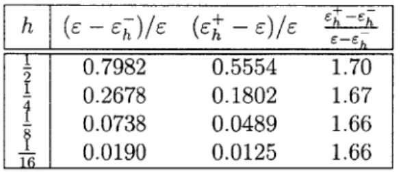
The computed bounds hold uniformly for any level of refinement, and in the asymp-totic convergence regime of the finite element method, the bound gap decreases at twice the rate of the 'H -norm measure of the error in the finite element solution. Given a finite element solution and its output adjoint solution, the method can be used to provide a certificate of precision for the output with an asymptotic complexity that is linear in the

4

number of elements in the finite element discretization. The complete procedure com-putes approximate outputs to a given precision in polynomial time. Local information generated by the procedure can be used as an adaptive meshing indicator. We apply the method to Poisson's equation and the steady-state advection-diffusion-reaction equation.

Thesis Supervisor: Jaime Peraire

5

Acknowledgments

First and foremost, I would like to thank my advisor, Professor Jaime Peraire, for his constant vision and continual supply of ideas, as well as for his encour-agement and patience during the course of this research. Second, I would like to heartily thank Professor Anthony Patera for taking me under his wing during my advisor's sabbatical and for introducing me to functional analysis in the context of the finite element method. I would like to thank everyone who participated in the "bounds sessions" organized by Professor Patera. In particular, I would like to thank Luc Machiels, Dimitrios Rovas, Ivan Oliveira, Karen Veroy, and Christophe Prud'homme for everything that they taught me as well as for their camaraderie. I would like to thank Professor Gilbert Strang for opening my mind to the underlying beauty of mathematics, and then Professor Dimitris Bertsimas to the underlying mathematical beauty of decision making. I would like to thank my committee as a whole, Professors Jaime Peraire, Anthony Patera, David Dar-mofal, and Dimitris Bertsimas for their helpful comments and insight. Further, I would like to thank Javier Bonet, Antonio Huerta, and Robert Freund for helpful discussions of various aspects of the method proposed in this thesis. As this work could not have been completed without financial support, I would also like to thank Thomas A. Zang for the support provided through NAG-1-1978 and the Singapore-MIT Alliance. I could not have overcome the many frustrations and disappointments experienced during the course of my studies without the unwa-vering support of my family and friends. I would especially like to thank my wife, Alexis, and my parents, Roger and Leslee Budge, whose constant love and encouragement renewed my strength when I thought that I could not continue. Finally, I would like to thank my Lord and Savior, Jesus Christ, for setting me free from a life of vanity and for teaching my heart, mind, body, and spirit not only about the wonders of grace, peace, faith, and hope, but about the very thing for which we were created- to love and be loved.

Contents

1 Introduction

1.1 Techniques for Reliability Assessment . . . . 1.1.1 Recovery Based Error Estimators . 1.1.2 Residual Based Error Estimators

1.1.2.1 Explicit Estimators . . . . . 1.1.2.2 Implicit Estimators . . . . . 1.1.2.3 Summary of Residual Based 1.1.3 Relation to Other Methods . . . . 1.2 Overview . . . . 2 Energy Bounds for Poisson's Equation

2.1 An Intrinsic Minimization Principle . . . . . 2.2 Weak Continuity Reformulation . . . . 2.3 Localization by Continuity Relaxation . . . 2.3.1 Continuity Multiplier Approximation 2.4 Local Dual Subproblem . . . .

2.4.1 Subproblem Computation . . . . 2.5 Energy Bound Procedure . . . . 2.5.1 Properties of the Energy Bound . . . 2.6 Numerical Results . . . . 3 Output Bounds For Poisson's Equation

3.1 Weak Continuity Reformulation . . . . 3.2 Localization by Continuity Relaxation . . . 3.2.1 Lagrange Multiplier Approximation . 3.3 Local Dual Subproblem . . . . 3.3.1 Subproblem Computation . . . . 3.4 Output Bound Procedure . . . . 3.4.1 Properties of the Output Bounds . . 3.4.2 Computational Complexity . . . . 13 . . . . 16 . . . . 17 . . . . 18 . . . . 19 . . . . 23 Error Estimators . . 26 . . . . 26 . . . . 28 30 . . . . 3 1 . . . . 32 . . . . 34 . . . . 34 . . . . 36 . . . . 39 . . . . 4 1 . . . . 4 2 . . . . 4 6 48 . . . . 4 9 . . . . 50 . . . . 5 1 . . . . 53 . . . . 55 . . . . 5 7 . . . . 59 . . . . 60 7

CONTENTS

3.5 Adaptive Refinement ... 62

3.6 Numerical Results ... 63

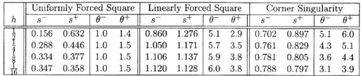
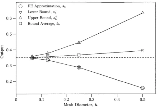
3.6.1 Uniformly Forced Square Domain . . . . 64

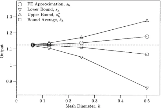
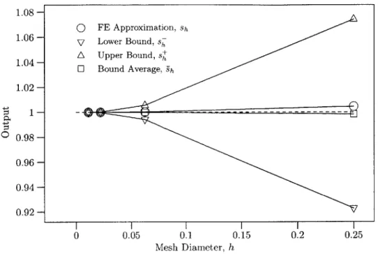
3.6.2 Linearly Forced Square Domain . . . . 65

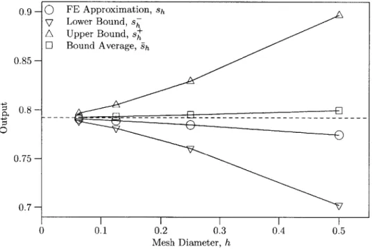
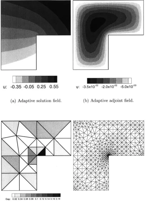
3.6.3 Unforced Corner Domain . . . . 68

4 Output Bounds for the ADR Equation 71 4.1 Constrained Minimization Reformulation . . . . 73

4.1.1 Weak Continuity . . . . 73

4.1.2 Operator Decomposition . . . . 74

4.1.3 Constrained Minimization Statement . . . . 75

4.1.4 Localization by Lagrangian Relaxation . . . . 76

4.1.4.1 Lagrange Multiplier Approximation . . . . 77

4.2 Elemental Subproblems . . . . 79

4.2.1 Dualization of Local Minimization . . . . 81

4.2.2 Dual Subproblems . . . . 84

4.2.3 Subproblem Computation . . . . 87

4.3 Output Bound Procedure . . . . 89

4.4 Numerical Examples . . . . 92 4.4.1 Quasi-2D Transport . . . . 93 4.4.2 Rotating Transport . . . . 96 5 Conclusion 101 5.1 Contribution . . . . 101 5.2 Recommendations. . . . . 104 A Equilibration Procedure 107 A.1 Problem Statement . . . . 107

A .2 Prelim inaries . . . . 108

A .3 Subproblem s . . . . 110 Bibliography

8

List of Figures

2.6.1 Uniformly forced square domain convergence history. . . . . 47 3.6.1 Uniformly forced square domain convergence history. . . . . 65 3.6.2 The dependency of flow rate through a viscous duct on channel

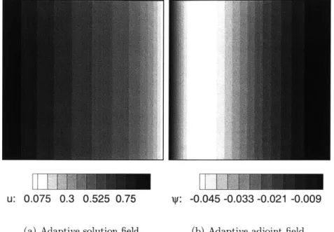
h eight. . . . . 66 3.6.3 Linearly forced square domain convergence history. . . . . 67 3.6.4 Unforced corner domain convergence history. . . . . 68 3.6.5 Unforced corner domain adaptive solutions, local indicators and

m eshes. . . . . 70 4.4.1 Quasi-2D uniform refinement results with q = 1, a = 10 and y = 10. 95 4.4.2 Quasi-2D transport adaptive solutions, local indicators and meshes. 98 4.4.3 Rotational transport forcing and output regions. . . . . 99 4.4.4 Rotating transport uniform refinement results. . . . . 99 4.4.5 Rotating transport adaptive solutions, local indicators and meshes. 100 A.3.1Equilibration subproblem interior case. . . . . 111 A.3.2Equilibration subproblem boundary cases. . . . . 113

List of Tables

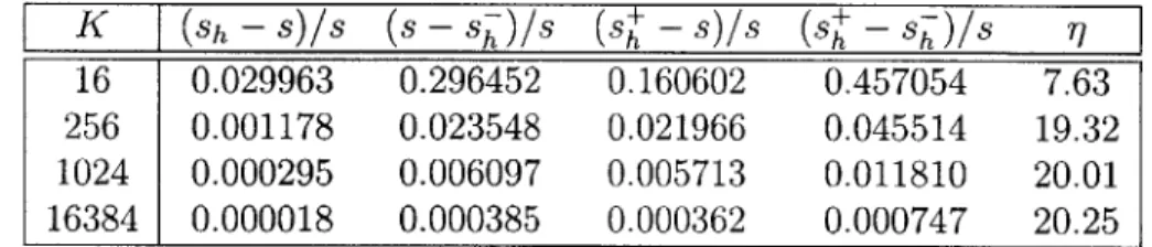
1.1 Error Estimator Methodology Conceptual Matrix . . . . 26 2.1 Uniformly forced square domain. . . . . 47 3.1 Output bounds and effectivities for three numerical test cases. . . 64 4.1 Quasi-2D uniform refinement results with q = 1, a = 10 and t = 10. 94 4.2 Quasi-2D uniform refinement results with q = 2 or 3, a = 10 and

y = 10 . . . . 95

4.3 Quasi-2D transport adaptive refinement results with p = 1 and various values of a. . . . . 96

Chapter 1

Introduction

Uncertainty about the reliability of numerical approximations frequently under-mines the utility of field simulations in the engineering design process: simula-tions are often not trusted because they lack reliable feedback on accuracy, or are more costly than necessary because they are performed with greater fidelity than necessary in an attempt to bolster trust. In addition to devitalized confidence, numerical uncertainty often causes ambiguity about the source of any discrepan-cies when using simulation results in concert with experimental measurements. Can the discretization error account for the discrepancies, or is the underlying continuum model inadequate?

To disambiguate, we define precision to be the conformity of a simulation re-sult to the exact solution of the continuum model, and we define accuracy to be the conformity of a simulation result to the physical fact. Three essential questions must be answered before a simulation result can be trusted and effectively used in the making important decisions. Do the mathematical equations model the rele-vant phenomena? Does the software actually solve the discretized mathematical

CHAPTER 1. INTRODUCTION

model? Does the simulation result contain sufficient precision to be considered a solution of the mathematical model?

The verification and validation process has emerged to help answer these ques-tions [AIA98, OT02, SWCP01]. Verification ensures that the simulation repro-duces known analytical results and trusted benchmarks, while validation ensures that the simulation results agree with trusted experimental data. The former con-firming that the simulation software solves the discretized mathematical model with sufficient precision for the verification test cases, and the latter substantiat-ing the capacity of the mathematical model to represent the relevant phenomena for the validation test cases. Verification and validation are necessary steps in assessing the reliability of simulation results, but these steps alone do not certify the accuracy of results for cases outside the test suite.

The reliability of every simulation result used in decision making should be taken into account, but it is often prohibitively expensive to do so. A priori error estimates inform us of the asymptotic rates of convergence, but cannot answer the ever present engineering question, "can I trust the current approximation?" Such questions often revolve around concerns of mesh fidelity and feature resolution

- issues of numerical uncertainty which erode confidence in the simulation. As confidence erodes, so does the utility of the simulation in the engineering design process: either the simulation is not trusted, or it is more costly than necessary.

While confidence in the precision of a field simulation can be buoyed by per-forming convergence studies, such studies are computationally very expensive and in practice are often not performed at more than a few conditions, if at all, due to cost and time constraints. For this reason, researchers and practitioners employ

15

adaptive methods to converge the solution in a manner that costs less in time and resources than uniform refinement. Adaptive methods powered by current error es-timation technology {Ver94, BKROO, BR78a, BSUG95b, BR96a, BBRW98, HR99, RS97, RS99, SBD+00, VD03, VD02], however, provide only asymptotic guarantees of precision, at best, and no guarantees of precision, at worse, since the conver-gence of adaptive methods remains an open question [MNS02, BV84, Dor96].

Our observations of engineering practice inform us that integrated quantities such as forces, total fluxes, average temperatures and displacements are frequently queried quantitative outputs from field simulations and that design and analysis does not always require the full precision available. In particular, we will restrict our attention to integrated outputs defined by linear functionals, which depend linearly on the solution field. The primary objective of our method, therefore, is to certify the precision of integrated outputs for low fidelity simulations as well as high fidelity simulations.

We call our bounds uniform to differentiate our goal of obtaining quantitative bounds for all levels of refinement from the lesser goal of obtaining quantitative bounds only asymptotically in the limit of refinement. In this regard, the com-plete procedure can be viewed as a polynomial time algorithm in the number of mesh elements that provides a certificate of precision for a predicted output. The certificate guarantees a minimum level of precision in the output from a particular finite-dimensional approximation with respect to the output from the

infinite-dimensional model that it is approximating. Furthermore, the procedure

provides local information that can be used in conjunction with adaptive meshing to efficiently drive a solution to an arbitrary and guaranteed precision.

CHAPTER 1. INTRODUCTION

The method can answer the question "Does the simulation result contain suf-ficient precision to be considered a solution of the mathematical model?" by certifying the precision of integrated outputs from finite element simulations for any level of mesh refinement. The method can help answer the question "Does the software actually solve the discretized mathematical model?" because it has eas-ily checkable preconditions to help verify correctness of the simulation software. The quantification of numerical error removes uncertainty about the fidelity of the discretization and aides the practitioner in distinguishing modeling error from numerical error when validating the simulation and thus can aid in answering the question "Do the mathematical equations model the relevant phenomena? ". In particular, the method can invalidate mathematical models when the error bounds returned by the method do not overlap with the experimental data. This can even be done with relatively low fidelity simulations in cases of gross deviation of the mathematical model from physical reality.

1.1

Techniques for Reliability Assessment

Verification and a posteriori error analysis have a long history in the development of the finite element method with a plethora of different approaches forwarded and investigated beginning with the pioneering work of Fraeijs de Veubeke in the mid-1960s and early 1970s [Fra64, Fra65, FH72]. Although powerful, his method was not practical because it required a global computation. In the late 1970s, Babuska and Rheinboldt initiated work on modern error estimation tech-niques by proposing the first inexpensive method requiring only local

computa-'R78a, BR78b, BR81]. Ainsworth and Oden giv ummary account of 16

1.1. TECHNIQUES FOR RELIABILITY ASSESSMENT

the work on a posteriori error estimators in [A097], while Babuska, Strouboulis,

Updahyay and collaborators probe the quality and robustness of a number of

con-temporary error estimators in [BSUG97, BSUG94, BSUG95a, BSU+94, ZSB01]

with numerical experiments. Additional comparisons and descriptions of the more

popular methods can be found in [ODRW89, Zhu97, SH98, AC92, Ver94].

1.1.1

Recovery Based Error Estimators

Finite element a posteriori error estimators can be broadly classified as recovery based methods or residual based methods, although evidence exists that some meth-ods which appear distinct under this categorization are equivalent [Zhu97, ZZ99] in special circumstances. Recovery based methods estimate the error in the energy norm by comparing the native finite element solution with one enhanced through a post-processing procedure. The post-processing procedure typically smoothes the finite element solution or exploits special superconvergent properties of the dis-cretization to obtain a recovered solution which is assumed to be more accurate than the original. Zienkiewicz and Zhu first proposed recovery based methods in the late 1980s [ZZ87] and have subsequently improved them [ZZ92a, ZZ92b] by ex-ploiting superconvergence. Recovery based methods have experienced popularity due to their simplicity as well as being very effective in practice [ZBS99, ZSBO1I].

Recovery based methods produce asymptotically exact error estimates when the post-processing produces a superconvergent recovered solution [CB02]. Asymp-totically exact error estimates converge to the exact error in the asymptotic limit of mesh refinement, but do not provide any guarantees of one-sidedness required for bounding the error. Asymptotic exactness is a very useful property for an error

CHAPTER 1. INTRODUCTION

estimator, but without uniform one-sidedness an error estimator cannot provide confirmation of precision. Even if the error estimator produces reliable estimates for a number of validation cases, there is little to assure the practitioner that the estimate can be trusted for the case of interest. Such limitations relegate the error estimator to serving as an oracle for balancing error contributions (of uncertain magnitude) in mesh adaptivity, and undermine their effectiveness as methods for confirmation and building adaptive meshes with guaranteed error tolerances.

1.1.2

Residual Based Error Estimators

Residual based methods, like the first locally computed error estimators which were introduced by Babuska and Rheinboldt, estimate the error in the energy norm either from an explicit evaluation of the local residual or by solving an implicit relationship with the local residual as the data. The majority of the work on error estimation has focused on residual based methods and the method proposed by this thesis can be categorized as such a method. Consider the simple model problem for an unknown real scalar field variable u and some nonnegative scalar coefficient y and data

f

posed on a two-dimensional domain

-Au + pU =

f

in Q C R2

subject only to homogeneous Dirichlet boundary conditions. The variational-weak statement follows as: find u in R'(Q)

a(u, v) = e(v), Vv E (1(1))

18

1.1. TECHNIQUES FOR RELIABILITY ASSESSMENT

where

a(u, v) = _{Vu - Vv + puv dQ,}

and

f(v)

=

jfvdQ.

The operator a : V(Q) x X-(Q) is symmetric, bilinear, continuous and coercive. We have introduced the usual Hilbert space

-H1()

=

{

v v E £2_{(Q), Vv E (E2(Q))d}

where d is the number of physical dimensions and

2 (Q V IV12

dQ <

+oo

is the space of square integrable functions on Q.

1.1.2.1 Explicit Estimators

Many of the first residual based a posteriori error estimators computed an error indicator explicitly from the approximate solution, without solving any additional problems [BR79, KGZB83, BM87]. Following Ainsworth and Oden [A097], we can build an explicit error estimator for the above model problem by the so called

error equation or residual equation

a(e, v) = a(u, v) - a(uh, v) = f(v) - a uh, v), VV E (1.()), 19

20

CHAPTER 1. INTRODUCTION

in which the error is defined as e

-

u - uh, where Uh E Vh is a finite element approximation to the solution on some triangulation of the domain, Th. The error

equation expands to

a(e, v) =

j

fV - VUhVV - IUhv dQ, Vv E

H'(Q).

T ETh T

Assuming Uh to be in H2(Q) and integrating by parts over the elements

decom-poses the error equation into local error contributions from each element

a(e, v) = E rvdQ - VUh -nv dF Vv (E H(Q),

T En E T

faT0

where r

f

+ Auh - pUh and n is the unit outward normal vector to 9Th. The

trace of v is continuous along an edge, which allows the last term of the previous equation to be written as the jump discontinuity in the approximation to the flux.

a(e, v) - rv dQ -

>

[Vuh -n] v dF, Vv E H1(Q),

TGThJ -Y9h\9 f

where

[VUa -

n]

= VuhIT+ -n + VUhT - = -R

is the jump discontinuity in the flux. We can now write

a(e, v) =Z rvdQ

+

Rv dl.

1.1. TECHNIQUES FOR RELIABILITY ASSESSMENT

Galerkin orthogonality, a(e, vh) = 0, Von E Vh, implies that

0 =

Zjrvv

dQ +

E

fRvhv dr,

TET -T E

where LVh

-H

1(T) -* Vh(T) is the linear operator that projects the members

of the infinite-dimensional continuous space, 7-(T), onto the finite-dimensional approximation subspace, Vh(T). We can subtract the previous two equations to obtain

a(e, v)

=

r(v

-

vhv)

dQ +

R(v

-

Hvhv) df, Vv E H (Q).

TET T Th J

Applying the Cauchy-Schwartz Inequality gives

a(e, v) ||r 1|2(T) I I Hv lVftI2(T) TETh

+ ||2 || - Hv oI L2(, Vv E XMG) yETh

Interpolation theory [Cia78, QV971 informs us that there exists a constant C which is independent of v and h, the diameter of the element, such that

l|v

- UvhvLe2 (T)

<

ChvI

7

-

(T*),

||v - flvhVllL 2(,) ChiVl(T*),

where T* denotes the subdomain consisting of all elements sharing a common edge with element T, and h is the diameter of T. Inserting these estimates into the

CHAPTER 1. INTRODUCTION

previous equation and absorbing the various constants, yields

a(e,v)

<

CjvfH1(Q)

h

2

|Ir|12

(T)

+

(

h||R||12h)}-TETh -YE a7h

Finally, recalling that IVol ( )

< a(v, v),

an a

posteriori

error estimate can be written

a(e,e)

C

{ h2||r|12(T) +

(

h||R|12)

.

T ETh -yE'Th

Both interior and edge residual quantities comprise the estimate, but in many situations the edge contribution dominates the estimate [KVOO, CV99].

Although simple, explicit error estimators of this sort have two obvious draw-backs. First and foremost, the estimate contains a generic unknown constant which renders the estimate useless for certifying the absolute precision of a nu-merical result. Second, the quantity on the right estimates the error in the energy norm measure which may or may not be relevant to particular decision for which the simulation was undertaken.

Linear Functional Output Error Measure An explicit estimator in a lin-ear functional output can be bootstrapped from the above energy estimator and an output adjoint. These estimators, of course, still contain unknown constants which make them unsuitable for confirmation and validation, but by serving as in-dicators for mesh adaptivity they can be used to improve the efficiency with which engineering quantities of interest can be approximated with greater precision.

Defining a linear continuous output functional f' : V -+ R. First, find Oh E Vh 22

1.1. TECHNIQUES FOR RELIABILITY ASSESSMENT

such that

a(0h, vh) = (Vh), Vo E Ph. 113

Galerkin orthogonality and the Cauchy-Schwarz Inequality allow us to write

EG(e) = a(e, @) = a(e, 0 - 0h) C e y~evh - IhJJvh, h1' (1.1.4)

where the solution error lJeJVh was obtained above. A bound on the term ||$

-Oh!IVh, where

4

E

H'(Q)

is the exact adjoint defined as

a(@, v)

= 0

(v),

Vv E

(),

can be obtained in an analogous manner to the solution error. This equation gives a lower bound, an upper bound can be found with the same process, but by

solving for -ED.

1.1.2.2 Implicit Estimators

The simplicity and low computational cost of explicit estimators makes them attractive despite their lack of quantitative feedback, while the quantitative po-tential of implicit estimators makes them attractive despite their additional cost. That implicit estimators are typically formulated without explicit constants, how-ever, belies the fact that the vast majority of such estimators tacitly depend on uncomputable quantities which must be approximated in a vitiating manner. As a result, existing implicit estimators cannot be used with confidence to validate the precision of a simulation result, despite the additional cost of such estimators. An implicit estimator for the error in a linear functional output can be con-23

CHAPTER 1. INTRODUCTION

structed from the error equation (1.1.2) using the approximate working solution Uh and the approximate adjoint Oh previously introduced. In order to reduce the computational cost of the resulting estimator, we introduce a domain decomposi-tion by partidecomposi-tioning the domain with the finite element trianguladecomposi-tion, Th. On the aggregate of elements, which we call the broken domain, we define a broken space V = HTETh 7

(T)

and a continuity bilinear form

b : V

x A constructed so that

V()

= {E V(Q) b(, A) = 0,

VA E

A

,

where A is the space of bounded linear edge functions (the dual of the trace space of

7-(T)).

Introducing the domain decomposition allows us to localize the error estimator computation to a single element.

After computing Uh and ih with standard methods, we can compute

equili-brating fluxes Au and A0 by solving the equations

b( , Au) =

E(0)

-

a(Uh, 0), VWE 4

b(0,A')

= - 0

(i)

-a(,@bh),

Vi

E Vh,

using well established and inexpensive equilibration techniques. Equilibrating

lo-calization techniques like this are an important ingredient to formulating robust

and asymptotically exact implicit error estimators [AO93a, Ain96, ABF99, A097,

BW851.

By choosing a high fidelity finite-dimensional approximation space V, (T) which we assume can safely be a surrogate for the infinite-dimensional space

N

1(T), we

1.1. TECHNIQUES FOR RELIABILITY ASSESSMENT

can solve a pair of high fidelity reconstructed error problems on each element

2a(eu, v) =

f(v)

- a(uh, v) - b(v,

Au),

Vv

E V,(T),

2a(el, v) = -E2(v) - a(v,'h) - b(v, AO), Vv E V,(T).

Upper and lower bounds on the output s - f 0(u) can then be computed from the

expression

s = 1i(u)

-

2 1: a(e',e) ± 2 ( a(e,er) 1

TGTh T E T T ET ) T

)

The quantities s* are quantitative bounds on the output from the hypothetical global high fidelity solution u,: s;- < 20_{(u) < s+.}

The method we have outlined here follows that of Patera, Paraschivoiu, Peraire, et al. [PPP97, PP98, MPP99, PPOO, BP02] in which the high fidelity approxima-tion space V, (T) is an h-refinement of the local element subdomain. As the method uses both a working mesh and "truth" mesh, it also falls under a category of two-level finite element methods studied by Brezzi and Marini [BM02]. Methods by other workers in the field have a similar character but use p-refinement for the local enriched approximation. Numerous implicit error estimation methods fall into this overarching scheme of computing high fidelity reconstructed errors from a localized working approximation. They differentiate themselves by the methods they choose for each step and how they measure the error. For instance, flux-free local problems may be computed on a patch of elements resulting from a partition of unity [MMPOO, BPP01], or the error might be measured with respect to the constitutive law [LadOO, LR97, LL83].

CHAPTER 1. INTRODUCTION

What the methods all have in common is substitution of a computable finite-dimensional problem where an uncomputable infinite-finite-dimensional problem is re-quired to guarantee bounds [AK01, A093b, BSG99, SBG00]. Error estimates that do not have the guarantee of one-sidedness, or that approach exactness but only in the asymptotic limit of either global or local problem resolution, cannot certify the precision of simulations posed on arbitrary meshes and require additional work to estimate the error in the error [SBG+99I.

1.1.2.3 Summary of Residual Based Error Estimators

Residual based error estimators like the ones introduced above can be viewed broadly with the conceptual matrix of Table 1.1. Notice that the proposed method targets the lower-right quadrant, which yields both greater utility (output metric) and greater rigor (implicit methodology).

Methodology

Metric Explicit Implicit

Babuska, Miller Bank, Weiser, Ladeveze, Energy RheinboldtVerfrth Leguillon, Babuska, Rhein-E el ,Verfrth boldt, Verffirth, Ainsworth,

Kelly, Gago Oe

Oden

Output Becker, Rannacher Patera, Peraire, et al.

Table 1.1: Error Estimator Methodology Conceptual Matrix

1.1.3

Relation to Other Methods

As the method presented in this thesis appeals to the dual of a minimization reformulation of the original problem, it can be conceptually viewed as an ex-26

1.1.

TECHNIQUES FOR RELIABILITY ASSESSMENT

tension of complementary energy techniques for error estimation, first proposed by Fraeijs de Veubeke [Fra65] in the early 1970s and later pursued by Lade-veze and Leguillon [LadOO, LL83, LR97, LRBM99], and others [Kel84, DM99],

to more relevant error measures and to problems without intrinsic minimiza-tion principles such as the advecminimiza-tion-diffusion-reacminimiza-tion equaminimiza-tion. Similarly, as the method solves equilibrated elemental residual subproblems, it can be concep-tually viewed as an extension of the work of Bank and Weiser [BW85], Ainsworth and Oden [A097, AO93b], and others [CKS99], which does not require exact min-imums of infinite-dimensional subproblems to guarantee bounds. Like Becker and

Rannacher [BR96a, BR96b, BKROO, RS98, RS97, RS99] and others [VD03, VD02],

we are interested in the precision of integrated output quantities and focus the adaptive refinement process on improving the precision of the desired output quan-tity in particular and not the solution in isolation.

In contrast to the work of Ladeveze, we endeavor to compute uniformly guar-anteed two-sided bounds on an output, not an estimate of the error in an abstract norm. While the work of Ainsworth and Oden as well as the related work of Cao, Kelly and Sloan [CKS991 require the exact solution of infinite-dimensional local problems in order to guarantee bounds, our method guarantees bounds uniformly with the solution of a finite-dimensional local problem. Our method differs from that of Destuynder in that it is not burdened with the explicit construction of globally conforming approximations to dual admissible vector fields and the local nature of our method readily provides an adaptive refinement indicator. More-over, the method introduced in this thesis extends to problems without intrinsic minimization principles such as the advection-diffusion-reaction equation.

CHAPTER 1. INTRODUCTION

Bertsimas and Caramanis have recently proposed a novel global method for computing bounds on functionals of partial differential equations using semidefi-nite optimization [BC02, BC00]. Like the method presented in this thesis, their method reformulates the output problem as an optimization problem. Initial nu-merical trials which included the non-coercive Helmholtz equation were promising but unfortunately the cost of performing the semidefinite optimization makes the method impractical at present.

Tangibly, the work presented in this thesis extends earlier work done by Pa-tera, Paraschivoiu, and Peraire [PPP97, PP98] on two-level residual based tech-niques for computing output bounds. The method presented in this thesis fol-lows the overarching scheme of this and other implicit methods, but transforms the local uncomputable indimensional subproblem into a computable finite-dimensional one and thereby retains the strong bounding property other methods loose. While the method has the very strong properties mentioned above which are not provided by other methods, it cannot yet be applied to curved domains or mathematical models with polynomial forcing and the extension to non-coercive equations is non-trivial.

1.2

Overview

In Chapters 2 and 3, we focus on the overarching structure of the method and do not consider the details of its implementation, nor more general equations such as non-symmetric dissipative operators, which will be presented in Chapter 4.

Chapter 2 presents the core concepts in the simpler setting of energy bounds for Poisson's equation, where the method has a clear variational meaning and a direct

1.2. OVERVIEW

relationship to hybrid methods. Chapter 3 recasts the energy bound method as a method for linear functional output bounds for Poisson's equation, simultaneously extending the energy bound to more relevant error measures and preparing the way for more general model problems. In Chapter 4 we generalize the method in a variety of ways while extending it to the advection-diffusion-reaction equation. Beginning with the description of the model problem and continued throughout the chapter, we give a more general presentation of the method which explicitly considers non-homogeneous boundary data. Numerical examples are given at the end of each chapter which demonstrate the potential for the method to deliver simulation results with certified precision.

Chapter 2

Energy Bounds for Poisson's

Equation

In the first two chapters we will consider Poisson's equation posed on polygonal domains, , in d spatial dimensions and, only for the sake of simplicity of pre-sentation, homogeneous Dirichlet boundaries, F = 8Q. The Poisson problem is formulated weakly as: find u E V such that

jVu - VvdQ = jfvdQ, VvEV, (2.0.1)

where V(Q) = { u E H'(Q)

I

ur = 0 } and the domain Q is assumed when

oth-erwise unspecified, that is, V = V(Q). As a consequence of all the Dirichlet boundaries being homogeneous, V serves as both the function set and test space in our presentation. While we present the method for homogeneous Dirichlet data, it can be easily extended to non-homogeneous data and Neumann boundary conditions.

2.1. AN INTRINSIC MINIMIZATION PRINCIPLE

2.1

An Intrinsic Minimization Principle

We begin by developing a lower bound on the total energy of the system,

j

fo

Vu-Vu dQ -

fn

fu dQ, which in the context of heat conduction, combines the heat dissipation energy, 1

fo

Vu -Vu dQ, and the potential energy of the thermal loads,

-

fn

fu dQ. There is a well known physical principle at work in this problem, related to the symmetric positive definite nature of the diffusion operator, which states that the solution, u, is the function that minimizes the total energy with respect to all other candidates in V

u = arg inf

j

Vw -VwdQ -

fwd,

(2.1.1)

as can easily be verified by comparing the Euler-Lagrange equation of this mini-mization statement to Poisson's equation (2.0.1). This minimini-mization formulation makes it clear that if we look for a discrete approximation of (2.0.1) in a finite set of conforming functions, Vh, for which Vh C V, then the resulting total energy predicted by the approximation will approach the exact value from above.

While insightful, this upper bound on the total energy has limited usefulness for two primary reasons. First, only rarely will the total energy be relevant to the purpose of solving the original problem. Second, even when it is relevant, the upper bound will most likely not be helpful for managing approximation uncer-tainty. In an engineering design task, the upper bound usually corresponds to the "best case scenario," as opposed to the "worst case scenario" which would be required to ensure feasibility of the design.

Our strategy for obtaining lower bounds on the energy in a cost efficient man-31

CHAPTER 2. ENERGY BOUNDS FOR POISSON'S EQUATION

ner is to first decompose the global problem into independent local elemental subproblems by relaxing the continuity of the set V along edges of a triangular partitioning of Q, using approximate Lagrange multipliers, then accumulate the lower bound from the objective values of approximate local dual subproblems.

2.2

Weak Continuity Reformulation

We begin by partitioning the domain into a mesh, Th, of non-overlapping open sub domains, T, called elements. The partition has the property UTEh T = Q, where the over-bar indicates the closure of the domain. We denote by BT the edges, -y, constituting the boundary of a single element T, and by

0Th

the network of all edges in the mesh. We have not yet evoked a discretization of V, but merely a domain decomposition represented by a mesh. With the broken space

S=

{

v E L

2_(Q)|v

ITE

'H(T),

VT

E Th

, (2.2.1)

in which the continuity of V is broken across the mesh edges, 0Th, we can re-formulate the energy minimization statement (2.1.1) by explicitly enforcing con-tinuity

u

=

arg inf

-fV

.

V& dQ -

f

b dQ

st

IV(2.2.2)

s.t.

1

ar TzA

dI' = 0, VA E A,

T67 Th

2.2. WEAK CONTINUITY REFORMULATION

where, for TN

C

Th and an arbitrary ordering of the elements,

T < TN,

-1 xETflTN,T<TN

0-T(X) = (2.2-3)

+1

otherwise.

Integrals over the broken domain, such as

fj

V* - V dQ, are understood as sums

of integrals over the subdomains, such as

EZT

fT VI T -Vi)H dQ. As there is no ambiguity, we have suppressed the trace operators from our notation for the boundary integrals to simplify the appearance of the expressions.

To see how the constraint arises, consider a single edge, 7 E 0Th, with

neigh-boring elements T and TN, for which a strong continuity constraint can be written roughly as ZbITO - I|TNy = 0 on

-y.

An integral weak representation is obtained by multiplying by an arbitrary test function,

A-,

taken from an appropriate space, A(7), integrating along the edge, and ensuring the resulting integrated quantity is zero for all possible test functions:

fY

(ZbT,- -

&I

TN,)

Ay

dl = 0, VAy

E

A(7).

The constraint used above is obtained by re-writing the combination of all edge constraints as a combination of elemental contributions, using oT to track the sign of the contribution. Since GlT is a member of H1(T), the trace of &iI on an edge -y is a member of H2

(OT).

Therefore, A on -y is a member of the dual of the trace space, H-21(7), and the continuity multiplier space A is the corresponding product space taken over all the edges of the mesh.

Notice that we have relaxed the Dirichlet boundary conditions as well as the interior continuity. The homogeneous Dirichlet conditions are weakly enforced implicitly by the continuity constraint. We shall not prove it here, but it is impor-tant to know that the minimizer of the constrained minimization problem (2.2.2) 33

CHAPTER 2. ENERGY BOUNDS FOR POISSON'S EQUATION

is indeed u, the exact solution of Poisson's equation (2.0.1) [A097, BF91].

2.3

Localization by Continuity Relaxation

Considering the Lagrangian of the constrained minimization (2.2.2),

L(j; A)

Vz - Vzb dQ-f

d-

T

o

T

d',

(2.3.1)

we recall from the saddle point property of Lagrange multipliers and the strong duality of convex minimizations that for all

I

E A

E- < inf L(ib;

I)

sup inf L(d; A) = _{inf sup L(b; A)} = E,

where the value at optimality is the minimum total energy of the continuum system, e = 2

fQ

Vu -Vu

dQ

-

fQ

f v

dQ. The lower bounding minimization for

a given

I

is separable, an important property allowing us to treat each element independently as will be discussed further in Section 2.4. In order to obtain a non-trivial (i.e. finite) lower bound, ~ cannot be chosen arbitrarily. We obtain A by approximating the problem using finite elements in a manner that guarantees the relaxed minimization is bounded from below.

2.3.1

Continuity Multiplier Approximation

We now introduce the finite element approximation of Poisson's equation (2.0.1) as means of obtaining an approximate Lagrange multiplier. We first solve the 34

2.3. LOCALIZATION BY CONTINUITY RELAXATION

finite-dimensional Poisson problem: find uh E Vh such that

j

Vuh

.-VvdQ

=

f

fvdQ,

Vv

E Vh,

(2.3.2)

where Vh-

{

v E V

I

vIT E PP(T), VT E T

}

for PP(T) the space of polynomials on element T (in d spatial dimensions) with degree less than or equal to p. Once we have obtained Uh, we solve the gradient condition of (2.3.1) to obtain Ah: find a Ah E Ah such that

-TOjAhd VUh -V dQ -

jf

dQ,

V

E

9h,

(2.3.3)

T ET

where Ah =

{

A E

A |

Alj

E

PP(y),

V'y

C

&T

}

for PP(y) the space of polynomials

on element edge -y (in d - 1 spatial dimensions) with degree less than or equal to p. We call this the equilibration problem, and we call any compatible Lagrange multiplier "equilibrating," since the problem has a non-unique solution. In the context of hybrid methods [BF91], this continuity multiplier is often referred to as a hybrid flux. As mentioned previously, this particular choice for the Lagrange multiplier ensures a finite lower bound.

Lemma 2.3.1. If a Lagrange multiplier Ah G Ah satisfies the equilibration

condi-tion (2.3.3), then

infEp

1

L(ib;

Ah)

is bounded from below.

Proof. Recall that the null space for the Laplace operator is the one dimensional

space of constants,

P

0, and let P0 =HTCTh P(T) denote the null space of the

broken operator. Considering 6 E IP C Vh in the equilibration problem (2.3.3) and that any zi

C

V

can be represented as '6 for fv' E

V

\#W0, it is easily shown that

C(&'

+

a;

Ah) = L('; Ah). For the Poisson equation, equilibration ensures 35

CHAPTER 2. ENERGY BOUNDS FOR POISSON'S EQUATION

that null space of the operator does not cause the minimization to be become unbounded below. The existence of a minimum now follows from the coercivity of the Poisson operator in

9

\

#P

0.

While not part of the classical finite element problem set, the equilibration problem has been addressed a number of times and in a number of contexts in the finite element community, not the least of which is in the context of error estimation [AO93a, LM96, MPOO]. The equilibration problem can solved with asymptotically linear computational cost in the number of mesh vertices and in some cases is already solved as a component of domain decomposition techniques for parallel computations [Par0l]. For our implementation, we use a method due

to Ladevaze [LL83, A097].

2.4

Local Dual Subproblem

Now that we have successfully decomposed the global problem into local elemen-tal subproblems, we can write the lower bounding minimization induced by the Lagrange saddle point property as

inf L(tb;

A)

=

inf

J(w)

7eV TG h wcV(T)

for

JT(w) -

jVw

-VwdQ

-

j

fwdQ

-

j Twl

dF,

(2.4.1)

and consider a representative minimization subproblem. The minimization sub-problem simply corresponds to a Poisson sub-problem of the type represented in

2.4. LOCAL DUAL SUBPROBLEM

tion (2.0.1) with Neumann boundary conditions posed on a single subdomain. We have done nothing to change the nature of original problem, but have only acted to decompose the global problem into a sequence of independent local problems. We do not require, and in general cannot compute, the exact minimum of the infinite-dimensional local subproblem, but we do require a lower bound for it and we proceed now to introduce the primary ingredient for obtaining this local lower bound.

Proposition 2.4.1. If we define the positive functional

JT(q) =j q - qdQ (2.4.2)

where q E 7H(div; T) and

H(div;

T)

={q

I

q

c

(L2_{(T))d, V}

_-

_q

_E

_L2_(T)}

_for

_a

problem posed in d spatial dimensions, then we have

JT(w) -Jr(q), Vw

C

H-1(T),

Vq E

Q(T),

(2.4.3)

for the set of functions

Q(T) {q

E

(div;T) jV-qvdQ-

q-nvdF

=-

fvdQ -

jA

vdf,

Vv

E'H1(T)}.

(2.4.4)

Proof. We begin by appealing to the following positive expression

f(q

Vw)2

dQ > 0,

ENERGY BOUNDS FOR POISSON'S EQUATION

for any w E ' 1(T) and any q E

Q(T).

This expression expands to

- _{q - qdQ}

+

-

_{Vw -VwdQ - j}

_{q -VwdQ > 0,}

in which we apply the Green's identity

-

q-Vwd=

jV-qwdQ- q-nwdF

to obtain

Iq - q dQ + _-12J_TVw -VwdQ +

_f

_V - qw dQ - q . nwdP > 0.

The constraint included in the definition of Q(T) makes this expression equivalent

to

[q - q + -

1d

T 2

IT

Vw -VwdQ -

_jfwdQ

-Identifying JT(w) and Jy(q) we arrive at the desired expression for the local lower

bound.

0

To obtain the best possible local lower bound, we might consider the following

maximization problem

sup -J (q) < inf JT(w),

qEQ(T) WEV(T)

with equality being obtained as a result of the convexity of JT and Jj.

(2.4.5)

1

aT Tw~dF

>

0.

(2.4.6)

38 CH APT ER 2.

2.4. LOCAL DUAL SUBPROBLEM

clear that we have derived a classic dual formulation1 for our local elemental minimization problem and essentially transformed a primal minimization problem into a dual feasibility problem. As we have alluded to earlier, the functional J (q)

is often called the complementary energy functional [QV97], when taken over the whole domain, Q, with a globally admissible complementary field.

2.4.1

Subproblem Computation

Significantly, we can make these subproblems computable by choosing an appro-priate finite-dimensional set in which to search for q. At the very least the set must be chosen so that the divergence of its functions contain the forcing function,

f,

in T and the normal traces of its functions contain the approximate continuity multiplier, Ah, on

&T.

In multiple dimensions, however, the polynomial approx-imation for the continuity multiplier will nullify any components of the set with non-polynomial normal trace. Therefore, we choose the polynomial approximation subset

Qh(T)

-{

q

E

(pq(T))d

V

-qvdQ

-

q -nvdF

JT J T

= -

f

vdQ

j

T

AhvdF, Vv

E I'(T) ,

(2.4.7) with q > p. As a consequence, the method as we have presented it is limited to forcing functions,

f

IT, that are perforce members of the polynomial space

P(T)

for q > r on each elemental domain. While in one dimension we gain no advantage

'The classic derivation for the dual of the Poisson problem would begin by letting q = Vw (a statement of Fourier's law in the context of heat conduction) and proceed by eliminating w from the problem.

CHAPTER 2. ENERGY BOUNDS FOR POISSON'S EQUATION

in taking q greater than r +1, in multiple dimensions we can do so in an attempt to sharpen the bounds. The interior constraint data,

f,

and the boundary constraint data, UTAh, cannot be chosen independently of each other, but must satisfy a

compatibility condition in order to ensure solvability as manifest by the following lemma.

Lemma 2.4.2. Suppose the forcing

function

f

T is a member of P(T) and that

Ah satisfies (2.3.3), then there exists at least one dual feasible

function,

q, that is

a member of Qh(T) for q p and q > r.

Proof. We begin by expressing q, a member of (Pq(T))d, as the combination

q = qD +q0, with qD a normal boundary condition satisfying component, qDn = UTAh on 0T, and q0 a homogeneous normal boundary condition satisfying com-ponent, q0 -n = 0 on 0T. With this lifting, we can write the feasibility constraint as

-jV-

q

0

vdQ=

jfvdQ+

V

-qDvdQ.

JT JT JT

Recognizing the divergence operator on the left hand side, which maps (Pq(T))d into Pq-l(T), we note that we need only test against v E P-1 (T). Furthermore,

finite-dimensional linear equations are solvable if and only if the right hand side data lies in the range of the operator, which is orthogonal to the null space of the adjoint operator. The adjoint operator is easily found to be fT q0 Vv dQ

which has the null space v E PO(T), and thus the right hand side data must be in Pq- I(T)

_{\ P0}

(T).-To prove solvability, we need only to verify that the right hand side data is orthogonal to the constants, since the requirements that q > p and q > r ensure that the right hand side data is in pq1. Choosing v = const in the right hand

2.5. ENERGY BOUND PROCEDURE

side of the constraint, rewritten as

j

f vdQ+

j

V

-qvdQ

=

f

vdQ

-

jqD

VvdQ+J

UTAhv

d,

reveals the compatibility condition

JT 0TAhdF = T

f

dQ,

(2.4.8)

which is satisfied by our choice for Ah, as can be seen by choosing v const on T in the equilibration condition (2.3.3). The equilibration condition thus ensures that the constraint data is compatible and that there exists at least one q satisfying the constraint.

2.5

Energy Bound Procedure

In discussing the global procedure and its properties, we denote the global ag-gregate of independent elemental quantities by accenting them with a diacritical hat as we did for the global broken quantities, and we denote the aggregate of local functional forms by dropping the subscript T. In particular, Qh denotes the aggregate approximate dual function space, 1TEh Qh(T), and Jc(ei) the aggre-gate dual energy functional,

ETTh

J (qlT). The complete method for the energy bounds consists of three steps:

1. Global Approximation: Find Uh E Vh such that

jVUh -

VvdQ = j

fvdQ,

Vv E

Vh,

(2.5.1)

CHAPTER 2. ENERGY BOUNDS FOR POISSON'S EQUATION

and calculate the upper bound E+ = -}

fa

Vh V h dQ.

2. Global Equilibration: Find )h G Ah such that

SIT

UTVAh

dF

= JVuh

-

V' dQ -

jf

d,

W

E

9h.

(2.5.2)

T ETh

3.

Local Dual Approximations:

Find e- such that

E = sup -J'(4h)

(2.5.3)

elhEdh

The last step requires the solution of a series of finite-dimensional quadratic programming problems with convex objective functions and linear equality con-straints. The per-element cost remains low due to the small size of the elemental subproblems, while the total cost of computing the lower bound is asymptotically linear in the number elements.

2.5.1

Properties of the Energy Bound

As previously discussed, the upper bound follows directly from the conforming nature of the finite element approximation and the lower bound follows directly from Proposition 2.4.1. We close our presentation of the energy bound method by showing that the lower bound converges at the same rate as the upper bound, and thus inherits the well known a priori finite element convergence property for the energy norm of the error. We begin by proving an orthogonality result.

Lemma 2.5.1. Let Oh be any dual

feasibility

correction to Vuh such that 4h =

2.5. ENERGY BOUND PROCEDURE

Vuh ±

Ph

is a member of Qh, then Ph satisfies the orthogonality property

S

Jp1

-V

v

dQ=0,

VVEh. (2.5.4) TETh T

Proof. We begin by examining the condition that the feasibility correction

Ph

must

satisfy by substituting Vuh + Ph into the constraint contained in the definition of

Qh, summed over the elements, to obtain

V

.Phib

dQ

- nJT - n dF=

-

f

f dQ -

V - Vhi)

dQ

TEn oT fn n

-o-rAsd

E+

VUh

-n dr, V

E

9.

(2.5.5)

T ETh TE h

Applying Green's formula to both the Ph and Uh terms yields the equivalent

constraint

jPh

-VbdQ =

fn

dQ -jVuh

-VbdQ+

I

o-rA dP, V' E

w

. (2.5.6) Restricting i to Vh produces the sought orthogonality property as a consequence

of equilibration (2.5.2).

L

Lemma 2.5.2. Let

Pi

be the dual feasibility correction to VUh that maximizes

Jc(Ph) such that Vuh + P* is a member of Qh, then

P*

is bounded

from

above

by

Jc(O*) < Clu - uhl,

(2.5.7)

for

the semi-norm Iv|=

fn

Vv

-

Vv dQ, if the approximate continuity multiplier