Revisiting the double checkpointing algorithm
Texte intégral
Figure
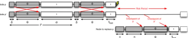
![Figure 1: Non-blocking checkpoint algorithm (see [2]).](https://thumb-eu.123doks.com/thumbv2/123doknet/14396141.509160/3.918.124.410.106.222/figure-non-blocking-checkpoint-algorithm-see.webp)
Documents relatifs
Mots clés : structures TCO, constantes optiques, épaisseurs, conception optimale, dominance, front de Pareto, cellules
Im Zusammenhang mit dem Traktat Christi Leiden ist nun zu fra- gen, wie dieser mit den in den Evangelien vorhandenen Anlagen ver- fa¨hrt und welche Schlu¨sse sich aus
In this paper, a new metaheuristic inspired by music improvisations, harmony search, is applied to solve the containers storage problem at the port. The
In the case of the Metropolitan Police Service in London, this has involved creating the Status Dogs Unit, an organisation populated by a group of police officers with a
It has two parts: first, we choose a migration strategy i.e the time slots where each tenant can migrate, and, second, we apply a heuristic using resources prices and capacity,
Meta-data describe job and job-unit related data and include: the kernel check- pointers used, the checkpoint version number, the process list, the process group reference id,
Unité de recherche INRIA Rennes, Irisa, Campus universitaire de Beaulieu, 35042 RENNES Cedex Unité de recherche INRIA Rhône-Alpes, 655, avenue de l’Europe, 38330 MONTBONNOT ST
Upon detection of a transient failure, if the last checkpoint is a memory checkpoint, all dirty active pages present in memory are discarded, pure recovery pages are restored
