GALOPR, a beam transport program with space-charge and bunching

HAL Id: in2p3-00546751

http://hal.in2p3.fr/in2p3-00546751

HAL is a multi-disciplinary open access archive for the deposit and dissemination of sci-entific research documents, whether they are pub-lished or not. The documents may come from teaching and research institutions in France or abroad, or from public or private research centers.

L’archive ouverte pluridisciplinaire HAL, est destinée au dépôt et à la diffusion de documents scientifiques de niveau recherche, publiés ou non, émanant des établissements d’enseignement et de recherche français ou étrangers, des laboratoires publics ou privés.

GALOPR, a beam transport program with space-charge

and bunching

B. Bru

To cite this version:

B. Bru. GALOPR, a beam transport program with space-charge and bunching. 3rd International Conference on Charged Particle Optics, Apr 1990, Toulouse, France. pp.27-34, �10.1016/0168-9002(90)90593-U�. �in2p3-00546751�

To be presented at the 3r d International Conference on Charged Particle Optics. Toalouse. April 24-27/04/1990

GALOPR. A BEAM TRANSPORT PROGRAM. WITH SPACE-CHARGE AND BUNCHING

Bernard BRU

GANIL - B.P. 5027 -14021 Caen Cedex - FRANCE

To be presented at the 3r d International Conference on Charged Particle Optics. Toulouse. April 24-27/04/1990

GALOPR. A BEAM TRANSPORT PROGRAM. WITH SPACE-CHARGE AND BUNCHING

Bernard BRU

GANIL - B.P. 5027 - 14021 Caen Cedex - FRANCE

GALOPR is a first order beam transport code including 3 dimensional space charge forces and the beam bunching process.

It deals with usual optical devices (bending magnets, lenses, solenoids, drift spaces, bunchers) and can take into account any special optical device represented by its transfer matrix with space charge (the "Muller" and the "Pabot-Belmont" inflectors were recently introduced as one of these devices). The beam can be continuous, bunched or undergoing a bunching or debunching process.

The beam line parameters can be optimized in order to fit any elements of the 6 x 6 transfer and/or covariance matrices in order to obtain the maximum transmission efficiency.

The results are presented with a complet set of print-outs and graphical displays. This code has been used to optimize the 100 kV Axial Injection Beam Line at GANIL.

1) Introduction

The computer code GALOPR (GAnil beam Lines OPtics including Radio frequency bunchers) has been developed at GANIL from the code PREINJ d>2>3)

which was written at CERN to study the focusing and bunching characteristics of the Low Energy Beam Transport system (LEBT) for the actual proton linac injector, including space charge forces.

Firstly, a version without buncher but allowing to choose the ion mass number and charge state was used at GANIL to calculate the transfer lines between the 3 cyclotrons.

This version included all the classical optics elements : drifts, quadrupoles, dipoles, solenoids, elements with a numerically known transfer matrix.

This computer code takes into account :

- one system composed of one or several bunchers, which creates the longitudinal emittance to obtain a bunched beam from a continuous beam,

- rebunchers (or debunchers) which behave as a thin lens both in the longitudinal plane and in the transverse planes,

- any elements which has an analytically known transfer matrix (as the Miiller inflector).

The beam is represented by an hyperellipsoid in the 6-dimensional phase space. All the forces (space charge forces included) are linear with respect to the reference particle, which remains energy fixed in the present version.

Whatever the couplings between the 3 phase planes of the beam, the space charge forces are calculated in the eigen-coordinates system of the real ellipsoid (bunched beam), then projected on the motion axes and added to the extend forces.

The beam transfer in a line with external conditions is rapidly calculated by the computer, using the matrix form.

In a reasonable time, several beam transfers can be calculated to adjust the external parameters (focusing or bunching).

To do so, we use an iterative method to fullfill conditions on the beam matrix and/or the transfer matrix at the end of the line and along the line. In such a way we can study the variation of the above parameters with the beam intensity and with the beam emittance. The search of these parameters makes it possible, either to adjust the tuning of an existing beam line or to study a new beam line which must fullfill some functions (for instance, to match the beam to a post accelerator).

A more accurate knowledge of the beam requires to use a "multiparticles" computer code, whiche uses as inputs the above calculated parameters and takes into account the non-linear forces due to space-charge and bunching elements. In this purpose, the computer code BUNCH^) has been developed at CERN to make comparisons with the linear computer code PREINJ. A new version of BUNCH (which does not include dipoles presently) has been developed at GANIL, to make comparisons with GALOPR, in order to study axial injections in injector cyclotron.

Both types of computer codes are complementary to study either an existing beam line or a new beam line.

2) Beam parameters

Each particle at a point S of the beam line is located in the 6-dimensional phase space by its coordinates : x, x* = dx/ds, y, y* = dy/ds, z, z' = dz/ds where S is the curvilinear coordinate. The fifth coordinate z_is proportional to the difference between the time of arrival of a particle at point S and the corresponding time to for the reference particle:

z = -vr(t-to) (1)

where Vr is the velocity of the reference particle.

The beam is entirely defined by its intensity and the second order moments of the particle distribution in the 6-D phase space ; we will sometimes call these moments "rms" values. They can be written, for a centered distribution :

uv with u, v e (x, x5, y, y\ z, z")

fv p(V)dV

(2)

where dV and V are the volume elements and the volume in the 6-D space.

If the 6 coordinates of each of the N particles of the distribution are known, the "rms" values become merely :

— 1 N

u v

4ç

(3)

and define the covariance matrix of the beam.

The type of distribution is assumed to be hyperellipsoïdal, i.e the surfaces of equal density are homothetic to the marginal hyperellipsoid £.

£ can be transformed into an hypeisphere S, having a radius R.

The volumic distribution function can be expressed by p(r) where r is the radius of an inner hypershere homothetic to S.

The volume element in a n-D hypeisphere is :

dV-nnr^dr (4) where £2n is the n-D solid angle (equal to the surface of a radius 1 hypershere).

The "rms" value according to one of the n coordinates in the hypersphere is :

u2 - 1 .

(5) The above expression makes it possible to calculate the ratio k between the marginal and the "rms" values for different types of distribution :

k = u

(6) where û is the maximum value of u coordinate, Eu and Eu are respectively the "rms" and marginal emittances in (u, u') plane.

As demonstrated by P. Lapostolle W and F. Sacherer W the evolution of the "rms" values depends mainly on the linear component of the space charge force, in the case of linear external forces. Therefore, all types of distributions having the same "rms" values can be treated by such linear programs ; the tuning of the physical parameters of the line is then the same for any distribution.

3) Space charge forces calculation

Both considered models, which describe the real space, take into account a uniform distribution (p(r) = est) in a n-D space, and lead to linear space charge forces. A continuous beam is represented by a infinitely long cylinder (n = 2, k = 2) and a bunched beam by an ellipsoid (n = 3, k = V5).

The components of the radial electric field inside an infinitely long cylinder with elliptical section are given by :

(7) and inside an ellipsoid by :

so

(8)

where a, b and c are the axes, if these volumes are in their principal axes and where :

So is the dielectric constant of vacuum

Pc and pe the charge density in the cylinder and in the ellipsoid.

T 1 . COO dX

Ja = j a b c J

° ( a2 + X)V(a2 + X) (b2 + X) ( c2 + X)

(9) and analogous for Jband Jc are form factors ; the elliptic integrals are numerically

computed by the Gauss'method.

Choosing s = v^ as the indépendant variable, the equations of motion can be written for both models :

d2x^ e

ds2 2£o(W/e)

(10) and same for equations y and z.

with W • energy per nucléon of the reference particle 6 = charge to mass ratio.

for the cylinder (same for y)

Soi-Kx * ^ , „ . . . Jx for the ellipsoid (same for y, z)

(12)

4) Transfer matrices

The beam line is composed of thick and thin elements ; the space charge forces act only in the thick ones, which are subdivided into steps, the length of which is chosen in such a way that it has only a small effect on the transverse dimensions.

4 types of transfer matrices, including space charge forces (except the first type) are defined for the different elements :

4.1. Thin elements

The transfer matrix for a pole-face rotation at one end of a dipole and for a rotation of the transverse coordinate system around the curvilinear coordinate are given in Ref.8.

Any element (or combinaison of elements) previously calculated and given in a numerical form (for instance, the Pabot-Belmont inflector) can be introduced in the program as a 6 x 6 matrix.

4.2. Thick elements with decoupled phase planes

If the reference frame of the ellipsoid and of the motion are the same, then the

space charge forces (Ku) can be added to the external ones (Qu) in each phase plane, leading to the Hill-type equation :

The following table gives the constants Qu corresponding to the external forces of

the different elements :

Element Drift space Quadrupole Solenoid(*) Rebuncher Qx 0 G/Br 1/2B«/Br T T V R T 2 ^ X ( W / e ) ^ Qv 0 -Qx Qx Qx Qz 0 0 0 - 2 Q x Br • magnetic rigidity

P X « Distance between 2 consecutive bunches adjacent

G • Quadrupole gradient (G > 0 is focusing in the x direction)

Bs - maximum field in the solenoid

V R T • maximum voltage times transit time factor on the axis L G * gap lenght for a single-gap element

Ls " solenoid length

In each phase plane, the 2 x 2 transfer matrix contains sine and cosine elements if Qu - Ku > 0 and cosh and sinh elements if Qu -Ku < 0.

4.3. Thick elements with coupled phase planes

We consider the most complicated case of a dipole with a bunch tilted with

respect to the axes. We first calculate the eigenvalues of the covariance matrix in the real space and the eigenvectors matrix [V] which transforms the (x, y, z) frame into the (X,Y,Z) frame of the ellipsoid; the "rms" values X2 , Y2 , Z2 of the ellipsoid are

the above eigenvalues.

According to the previous paragraph, the space charge constants Kx, Ky and Kz can be calculated.

The new 6-D covariance matrix may be obtained in two ways.

(*) A rotation by an angle Qx Ls must be added afterwards to get the transfer matrix in

First method

The 6-D covariance matrix is calculated in the (X, Y, Z) frame ; then, a new one is obtained by the action of a thin lens with a strength equivalent to the effect of the space charge force over one step.

This new matrix is projected on the original reference frame, and is finally transfered through the next element step.

Second method

The forces KXX, KyY and KZZ are projected on the original axes, giving :

FyU[v]-l

LFzJ

system : JL Id? • p 2X-pd s t - S - y - 0 P2 dfo m ]_ dx " « ds (15)

with n - field index

p = radius of curvature of the reference frame

And the resulting system is solved by classically going to a Runge-Kutta method applied to a six first-order differential equations system.

The final transfer matrix is composed of the 6 vectors, solutions of the system. It is however necessary to perform a matrix transformation at both ends in order to take into account the difference between entrance and output reference frames.

Presently, only the second method is programmed ; indeed, it seems more physical to add the forces before solving the differential equations.

4.4. Special elements

The Miiller inflector in one of them^ : it can be represented by an analytical transfer matrix, expressed in a coordinates system associated to the electric field, from the origine to any point inside. The space charge effect is taken into account by adding a perturbation matrix to the matrix without space charge.

Pratically, we calculate the transfer matrix for the whole inflector, for a 90° deflection angle. Since the inflector is attached to the central region of a compact cyclotron, two additionnai effects must be taken into account : the magnetic field rising during the pole crossing and a rotation of the inflector coordinates-system to match the referency coordinates-system of the accelerated motion in the cyclotron.

5. Transition from a continuous to a bunched beam

All the elements studied above have a linear action on the beam. When a continuous beam, with a negligible energy spread, traverses a buncher, the energy modulation resulting from the sinusoidal voltage generates a longitudinal emittance. In our model, it is of importance to include in this emittance only the particles that will be captured further while taking into account the effect of all the particles (including those which will be lost) for the space charge force calculations. We proceed in 3 steps : 5.1.Generation of the longitudinal emittance at the buncher

a) Case of a fundamental buncher alone

Before the buncher, the emittance is a single line along the phase axis (zero energy spread). The relative momentum spread is given by :

_ „ sin(2jr—) P 2(W/s) pX

(16) The assumption is that, at the buncher, the trapped particles lie inside the hatched region of figure 1 ; the separation between the trapped and rejected particles is called the

ongiiudind emiitance

buncher RF voltage

region of accepted particles

Model chosen at the buncher to uass from a continuous beam to a bunched beam.

Since at this point, the beam is continuous, the trapped part is proportional to 4>c :

where i<> is the current upstream.

n = cfe fa is the "bunching efficiency".

In order to inject this bunch into the following sections of the line, the hatched portion of the cylinder is modified into an ellipsoid with the same volume and the same "rms" values x and y.

The marginal ellipsoid, supposed to be uniformly charged, has the following semi-axes :

and cpe

lit 'lit

The ratio 6/5 comes from the equality of the volumes. The "rms" values in the longitudinal plane can be calculated analytically by taking as a distribution, either the ellipsoid between • <pe and + cpe or the hatched cylinder between - cpc and + cpc d>2).

The modulation represented on figure 1 is only an approximation ; in fact, the modulation depends also on the radial position of the particle (a particle outside the axis

gain more energy than a particle on the axis) and is given by the radial variation of the transit time factor :

T0) = ToI o ( k r r ) - T o ( l + ( ^ - ; y2))

(17) where r, x, y are the transverse coordinates of the particle.

The second order momenta are then calculated analytically, by integrating not only the phases between -<Pc and + <pc, but also the radii between 0 and r, the

distribution being uniform in the real ellipsoid (3). b) Case of a multi-bunchers system

The modulation curve 5p/p = f(<p) can fit a linear curve (so, the longitudinal emittance decreases for a given cut-off phase) by adding one or several sinusoidal voltages, obtained from one or several bunchers working on an harmonic, multiple of the first one. The determination of the second order momenta, which becomes analytically impossible, is then calculated numerically, by applying the bunchers modulation to a certain number of particles in the plane (cp,5p/p), taken equidistant on the phases axis between -it and +TT, before bunchers effect.

When all bunchers have behaved, the modulation curve is obtained point to point. In this computer code, this method is applied for a 2 bunchers system, the second one working with a frequency, double of the first one.

a) b & * , A<t>, AW Z

AN

V

Fig.2 : Energy modulation vith a Double Drift Harmonic Buncher IDDHB^. a) Modulation curve of 1s t buncher : £3t^ - - eVBT sin

b) 1: transformed modulation curve of the 1s t buncher :

- *1 2 sin vith

2: modulation curve of 2n d buncher : c) Modulation curve of the DDHB system.

*

" g x

•VBT0 312

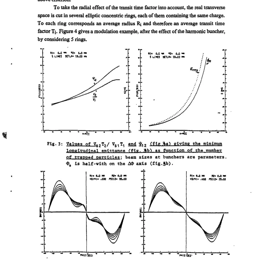
In this case, 2 tuning parameters can be adjusted, for a given cut off phase and a given voltage on the first buncher : the distance di2 between the bunchers gaps and the maximum voltage VB2 given by the second buncher, to obtain the minimal longitudinal emittance ; this gives an optimal modulation in this emittance (Figure 3). When the distance di2 is fixed (bunchers existing), only the voltage VB2 is adjusted according the above criterion.

To take the radial effect of the transit time factor into account, the real transverse space is cut in several elliptic concentric rings, each of them containing the same charge. To each ring corresponds an average radius Rj and therefore an average transit time factor Tj. Figure 4 gives a modulation example, after the effect of the harmonic buncher, by considering 5 rings.

su s.e -» v> «.a i

Î LINE: xv.n- <j.2o i HI* S.C >w « • 6.0 • •_{S tlitS mi*' 5S.2S m}

Fig. 3: Values_of_V82T2/ VB1T-, and longitudinal emittance (fig.

(fig -%a^ giving the minimum as function of the number1 of trapped particles: beam sizes at bunchers are parameters. <£, is half-with on the &P axis (fig.5b).

NI« 1.0 m .sea « • a.o m 3s.sa m * «.a m n> 8.o m .100 nUZ- 25.SS

In the computer code, this method is used also in the case of one buncher, where distance dn and voltage VB2 ate simply equal to zero.

5.2. Longitudinal adjustment without space charge

In the preceding section we have chosen arbitrarily the cut-off phase and the voltage on the first buncher.

In the case of an acceptance ellipsis in his principal axis at the matching point, the value Acpa of the acceptance in phase corresponds to the intersection of the ellipsis with the phases axis (figure 1). This value depends only on the given phase <pc. In the case of

two bunchers, we must adjust the distance â\2 and the voltage V^2 according to the criteron described in the preceding section. Then we have only to adjust the \ Itage VBI to get the ellipsis in its principal axes.

5.3. Introduction of the space charge

We have to fullfill the following requirement ; there must be continuity of the space charge forces during the transition from a 4-D to a 6-D phase space.

The chosen model is a combination of the actions of an infinite cylinder with the density pc of the rejected particles and of an ellipsoid with the density pc . Pe» where pe

is the density of the trapped particles. These densities are given by :

V ( 1

-(18) with Vo= 4;rjîX x y = volume of the cylinder having the lenght BX

and V * Su x y z = volume of the hatched cylinder and can be replaced in formulae (11) and (12), giving :

Same for Ky

K Z - K | - p e'p c jg

z 2eo(W/e) Z

(19) 6. Optimisation of the transport line parameters

The matrix formalism described precedently allows the transfer of a beam of charged particles with or without space charge effect. The purpose of this code is to determine the tuning parameters of the beam transport line.

6.1. Transfer planes adjustment

The parameters aie : the gradient of the quadrupoles and more rarely the length of the drift spaces.

The conditions imposed in one point of the beam line can be :

- on the covariance matrix elements of the beam (envelope, inclination of the emittance ellipsis or other correlation), at the matching point,

• on the transfer matrix elements (achromatism in position and in angle at a given point, focusing point,...).

The constraints in the transverse planes can be imposed by the limitation of the envelope along the beam transport line (say before or after a buncher) or in same given point of the transport line (diaphragm).

When taking into account the space charge effect (these forces are included in the transfer matrix), the conditions for the beam matching are imposed only on the covariance matrix elements. In the case of a beam with phase planes completely decorrelated at the entrance of the transport Une, the beam achromatism can be acheive in position and angle at a given point if we put these such matrix elements, 051, 052,0(,i and (J62 to zero.

6.2. Longitudinal plane adjustment

The cut-off phase cpc and the voltage of the first buncher can be changed in such a way that we can obtain the right acceptance in phase and the right inclination angle of the longitudinal ellipsis at the end of the transport line. Furthermore, if we place a rebuncher after the bunching system, we can impose a third condition : an energy dispersion or a given phase spread at the rebuncher.

6.3. Coupling between phase space planes

Due to the fact that we can have different coupling between transversal planes on one hand and the longitudinal plane on the other hand, it was necessary to include all the parameters and all the constraints in the same optimisation step.

6.4. Minimization method

The minimization is done using the least square method. The n variables are the

different parameters and the m functions, fj (xi, X2, ...Xn) correspond to the various conditions and constraints given by the beam transfer.

The method consists in doing the sum of the square of the m functions multiplied by their proper weight and then to find the parameters that minimize this sum (-l(i\

m

,X2i ...»

.I^frw

7. Typical example

An illustration of the use of the programm is given in the case of the 100 kV Axial Injection for the CO1 cyclotron at GANIL (O.A.I. project^^.The layout of the injection line and the corresponding beam envelopes are shown in figures 5 and 6.

8. Conclusion

The code GALOPR is now running onto the IBM 3090 (VM/XA system) of the C2 IN2P3 (IN2P3 computer center in Lyon) and onto the 32 bits MODCOMP at GANIL. An off-line code allows to draw the beam envelopes onto a "BENSON" plotter or a laser printer. A french notice (12) describes the code. It is distributed by the Los

Alamos Accelerator Code Group (LAACG).

Two further improvements to this code are planed by introducing : - the first method described in § 4.3,

- elements in which the central particle is accelerated. References

(1) - B. BRU and M. WEISS, CERN/MPS/LIN 72-4 (1972).

(2) - M. WEISS, Proceeding of the particle Conference San Fransisco, 1973 • IEEE NS20, n°20, n°3 p.877.

(3) - B. BRU, M. WEISS, CERN/MPS/IIN 74-1 (1974).

(4) - B. BRU, Proceedings of the EPAC, ROME, 1988 - n°l, p. 660. (5) - B. BRU, D. WARNER, CERN/MPS/LIN 75-2 (1975). (6) - P. LAPOSTOLLE, CERN/ISF/DL70-36 (1970). (7) - F. SACHERER, CERN/S/DL/70-12 (1970).

(8) - K.L. BROWN, D.C. CAREY, Ch. ISELJN and F. ROTHACKER, CERN/80/04. (9) - R. BECK, B. BRU and Ch. RICAUD, GANIL A86-02 a et b (1986).

(10)-.T.POMENTALE,CERNPrCi _ library, D507 (1968).

(11)-R.BECK,S.CHEL,B.BRU< J RICAUD, Proceedings of the: BERLIN (1989)

Dh/'ecf ûDf'/it

Caption: OA = transverse betatron matching AB = horizontal chromatic macching BC = vertical chromating aacching CD = transverse correlation matching DC - infleccor + el.-stat. quadrupole

Sola, note/ £5 Quad Aistchinct /tomt " J * . Inf/aefar gnfrsneo. S. JnF/ncfgr <zx.it \

Fig. 5: General layout of the

L. D M . FIX. NC01 H3 DU PT OBJ fl NC01 I N F . PB 0/20 3 . / 3 . 1GDH -21/10/88 10.15.34 EM-H= 56.00 EM-V= 56.00 MM»MRD DM/H= 0.050 PM

S