HAL Id: hal-00491292
https://hal.archives-ouvertes.fr/hal-00491292
Submitted on 11 Jun 2010
HAL is a multi-disciplinary open access
archive for the deposit and dissemination of
sci-entific research documents, whether they are
pub-lished or not. The documents may come from
teaching and research institutions in France or
abroad, or from public or private research centers.
L’archive ouverte pluridisciplinaire HAL, est
destinée au dépôt et à la diffusion de documents
scientifiques de niveau recherche, publiés ou non,
émanant des établissements d’enseignement et de
recherche français ou étrangers, des laboratoires
publics ou privés.
Schwarz Waveform Relaxation Methods for Systems of
Semi-Linear Reaction-Diffusion Equations
Stephane Descombes, Victorita Dolean, Martin Gander
To cite this version:
Stephane Descombes, Victorita Dolean, Martin Gander. Schwarz Waveform Relaxation Methods for
Systems of Semi-Linear Reaction-Diffusion Equations. 2010. �hal-00491292�
Schwarz Waveform Relaxation Methods for
Systems of Semi-Linear Reaction-Diffusion
Equations
St´ephane Descombes1, Victorita Dolean1 and Martin J. Gander2
1 Universit´e de Nice Sophia-Antipolis, Laboratoire J.-A. Dieudonn´e, UMR CNRS
6621, Parc Valrose, 06018 Nice 02, France, [email protected]
2 Universit´e de Gen`eve, Section de Math´ematiques, CP 64, 1211 Gen`eve,
Summary. Schwarz waveform relaxation methods have been studied for a wide range of scalar linear partial differential equations (PDEs) of parabolic and hyper-bolic type. They are based on a space-time decomposition of the computational domain and the subdomain iteration uses an overlapping decomposition in space. There are only few convergence studies for non-linear PDEs.
We analyze in this paper the convergence of Schwarz waveform relaxation applied to systems of semi-linear reaction-diffusion equations. We show that the algorithm converges linearly under certain conditions over long time intervals. We illustrate our results, and further possible convergence behavior, with numerical experiments.
1 Introduction
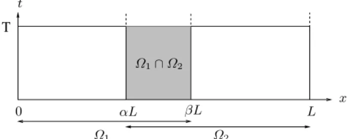
Schwarz waveform relaxation methods are domain decomposition methods for evolution problems, which were invented independently in [1, 6], and [7], where the latter paper only appeared several years later in print. These methods use a domain decomposition in space, and a subdomain iteration in space-time to converge to the underlying time dependent solution, see Figure 1 for an illustration. Schwarz waveform relaxation methods exhibit different conver-gence behaviors, depending on the underlying PDE and the time interval of the simulation: for the heat equation, convergence is linear over long times, see [6], and superlinear over short times, see [7]. For the wave equation, con-vergence is obtained in a finite number of steps for bounded time intervals, see [4], where also an optimized variant is described, which was first proposed in [3], both for hyperbolic and parabolic problems.
The analysis of Schwarz waveform relaxation methods for nonlinear lems is significantly more difficult: for scalar semilinear reaction diffusion prob-lems, see [2], and for scalar convection dominated nonlinear conservation laws, see [5]. The purpose of our paper is to present a first convergence analysis for
2 St´ephane Descombes, Victorita Dolean and Martin J. Gander
systems of nonlinear PDEs, for the model problem of semilinear reaction dif-fusion equations.
2 Systems of Semi-linear Reaction Diffusion Equations
To simplify the presentation, we show our results for a system of two equa-tions in one spatial dimension, but the techniques used in the analysis can be generalized to systems with more unknowns, and also to higher dimensions. We consider on a bounded domain Ω ⊂ R the system of semi-linear reaction diffusion equations
∂tu− ∆u + f(u) = 0 in Ω × (0, T ),
u(x, t) = g(x, t) on ∂Ω × (0, T ), u(x, 0) = u0(x) in Ω,
(1) where u = (u1, u2) represents the vector of two unknown concentrations to be
determined, and f(u) = (f1(u1, u2), f2(u1, u2)). A well posedness result for
such systems of semi-linear reaction diffusion equations can be found in [8], see Corollary 3.3.5, page 56.
Our analysis of the Schwarz waveform relaxation algorithm is based on comparison principles. Such principles have been studied in various contexts for system (1), see for example [10], [11], and they often require quite elaborate proofs for the generality employed. We state here precisely the results we need. Lemma 1. Let u = (uj)1≤j≤2 ∈ C2,1(Ω × [0, ∞))2 be a function for which
each component satisfies the inequality
∂tui− ∆ui+ ai1(x, t)u1+ ai2(x, t)u2> 0 in Ω × (0, ∞),
ui(x, t) > 0 on ∂Ω × (0, ∞),
ui(x, 0) > 0 in Ω.
(2) If aij(x, t) ≤ 0 for i '= j and all (x, t) ∈ Ω × (0, ∞), then ui(x, t) > 0 for all
(x, t) ∈ Ω × (0, ∞).
The proof of this theorem by contradiction is a straightforward extension of the result in the scalar case, see [2]. The strict inequalities in Lemma 1 can however be relaxed, as we show next.
Lemma 2. Under the same assumptions as in Lemma 1, if ∂tui− ∆ui+ ai1(x, t)u1+ ai2(x, t)u2≥ 0 in Ω × (0, ∞),
ui(x, t) ≥ 0 on ∂Ω × (0, ∞),
ui(x, 0) ≥ 0 in Ω,
(3) then ui(x, t) ≥ 0 for all (x, t) ∈ Ω × (0, ∞).
Proof. By performing the change of variables ˜ui(x, t) := eCtui(x, t), where C
is a constant to be chosen, the first inequality of (3) can be rewritten as ∂t˜ui− ∆˜ui− C ˜ui+ ai1˜u1+ ai2˜u2≥ 0. (4)
Now let ˆu = ˜u + ε. If we rewrite (4) in terms of ˆu, and choose the constant C such that C < ai1+ ai2, we can apply Lemma 1, and taking the limit for
ε→ 0 shows that ui(x, t) ≥ 0.
3 Schwarz Waveform Relaxation Algorithm
We consider the semi-linear reaction diffusion system (1) in the domain Ω = (0, L). We decompose the domain into two overlapping subdomains Ω1 =
(0, βL) and Ω2= (αL, L), α < β, as shown in Figure 1. We denote by g1(t) :=
T x t Ω1∩ Ω2 Ω1 Ω2 0 αL βL L
Fig. 1. Space-time domain decomposition.
g(0, t) and by g2(t) := g(L, t). The classical Schwarz waveform relaxation
algorithm constructs at each iteration n approximate solutions vn, wn on
subdomains Ωi, i = 1, 2, by solving the equations
∂tvn+1− ∆vn+1+ f(vn+1) = 0 in Ω1× (0, T ), vn+1(0, t) = g 1(t) on (0, T ), vn+1(βL, t) = wn(βL, t) on (0, T ), vn+1(x, 0) = u0(x) in Ω1 ∂twn+1− ∆wn+1+ f(wn+1) = 0 in Ω2× (0, T ), wn+1(αL, t) = vn(αL, t) on (0, T ), wn+1(L, t) = g 2(t) on (0, T ), wn+1(x, 0) = u 0(x) in Ω2. (5)
In order to analyze the convergence of the Schwarz waveform relaxation algo-rithm (5) to the solution u of (1), we denote the errors in subdomain Ω1 by
dn := u − vn and in Ω
4 St´ephane Descombes, Victorita Dolean and Martin J. Gander ∂tdn+1− ∆dn+1+ f(u) − f(vn+1) = 0 in Ω1× (0, T ), dn+1(βL, t) = en(βL, t) on (0, T ), ∂ten+1− ∆en+1+ f(u) − f(wn+1) = 0 in Ω2× (0, T ), en+1(αL, t) = dn(αL, t) on (0, T ), (6)
where the initial and boundary conditions on the exterior boundaries are zero, since the error vanishes there. Using a Taylor expansion with remainder term in Lagrange form, we obtain for i = 1, 2
∂tdn+1i − ∆dn+1i + ∂1fi(ξi,1, u2)dn+11 + ∂2fi(v1n+1, ξi,2)dn+12 = 0 in Ω1× (0, T ),
∂ten+1i − ∆e n+1
i + ∂1fi(ξi,1" , u2)en+11 + ∂2fi(wn+11 , ξi,2" )en+12 = 0 in Ω2× (0, T ),
a linear system with variable coefficients, depending on the Jacobian of the non-linearity.
Our convergence analysis is based on upper solutions for the errors, which are constant in time.
Theorem 1 (Linear Convergence Estimate). Assume that ∂1f1≥ 0 and
∂2f2 ≥ 0, and that there exists a constant a satisfying 0 < a < (π/L)2, such
that −a ≤ ∂1f2 ≤ 0 and −a ≤ ∂2f1 ≤ 0. Then the errors in the Schwarz
waveform relaxation algorithm (5) satisfy sup x∈Ω1*d 2n+1(x, ·)* ∞≤ C1γk*e0(βL, ·)*∞, (7) sup x∈Ω2*e 2n+1(x, ·)* ∞≤ C2γk*d0(αL, ·)*∞, (8) where γ in (0, 1) is γ =! sin(√aαL) sin(√aβL) " ! sin(√a(1 − β)L) sin(√a(1 − α)L) " , and the constants C1,2 are given by
C1= sup 0<x<βL sin(√ax) sin(√aβL), C2= sup αL<x<L sin(√a(L − x)) sin(√a(1 − α)L). Proof. Let M := max {||en
1(βL, ·)||∞,||en2(βL, ·)||∞} and define the function
˜
dn+1 := M sin(√ax)/ sin(√aβL), which is the unique solution of the steady
state problem
−∆ ˜dn+1− a ˜dn+1= 0, with ˜dn+1(0) = 0, d˜n+1(βL) = M. In order to show that ˜dn+1is a supersolution of the two errors dn+1
1 and dn+12 ,
we consider the differences ˆdn+11 := ˜dn+1− dn+11 and ˆdn+12 := ˜dn+1− dn+12 ,
which satisfy in Ω1the system of equations
∂tdˆn+11 − ∆ ˆd1n+1− a ˜dn+1− ∂1f1(ξ1,1, u2)dn+11 − ∂2f1(vn+11 , ξ1,2)dn+12 = 0,
Adding and subtracting ∂1f1(ξ1,1, u2) ˜dn+1 and ∂2f1(v1n+1, ξ1,2) ˜dn+1 in the
first equation, and ∂1f2(ξ2,1, u2) ˜dn+1 and ∂2f2(v1n+1, ξ2,2) ˜dn+1 in the second
equation, we obtain
∂tdˆn+11 − ∆ ˆdn+11 = −∂1f1(ξ1,1, u2) ˆdn+11 − ∂2f1(vn+11 , ξ1,2) ˆdn+12
+∂1f1(ξ1,1, u2) ˜dn+1+ (a + ∂2f1(vn+11 , ξ1,2)) ˜dn+1,
∂tdˆn+12 − ∆ ˆdn+12 = −∂1f2(ξ2,1, u2) ˆdn+11 − ∂2f2(vn+11 , ξ2,2) ˆdn+12
+(a + ∂1f2(ξ2,1, u2)) ˜dn+1+ ∂2f2(vn+11 , ξ2,2) ˜dn+1.
Under the assumptions of the theorem, and using the fact that ˜dn+1is strictly
positive in the interior of subdomain Ω1, we obtain the system of inequalities
∂tdˆn+11 − ∆ ˆd n+1
1 + ∂1f1(ξ1,1, u2) ˆdn+11 + ∂2f1(vn+11 , ξ1,2) ˆdn+12 ≥ 0,
∂tdˆn+12 − ∆ ˆd2n+1+ ∂1f2(ξ2,1, u2) ˆdn+11 + ∂2f2(vn+11 , ξ2,2) ˆdn+12 ≥ 0.
Since ∂2f1(v1n+1, ξ1,2) ≤ 0 and ∂1f2(ξ2,1, u2) ≤ 0, we can now apply Lemma 2
to conclude that ˆdn+11 = ˜dn+1− dn+11 ≥ 0 and ˆdn+12 = ˜dn+1− dn+12 ≥ 0 in Ω1.
Using a similar argument for the sums, we obtain that also ˜dn+1+ dn+1 1 ≥ 0
and ˜dn+1+ dn+1
2 ≥ 0, which implies by the positivity of ˜dn+1 that their
modulus is bounded, and we have for i = 1, 2 |dn+1
i (x, t)| ≤ ˜dn+1= max {||en1(βL, ·)||∞, ||en2(βL, ·)||∞}
sin(√ax) sin(√aβL). Using a similar argument on subdomain Ω2, we obtain for i = 1, 2
|en+1
i (x, t)| ≤ max {||d n
1(αL, ·)||∞,||dn2(αL, ·)||∞}sin(√a(1 − α)L)sin(√a(L − x)) .
Since the bounds are uniform in t, we obtain over a double step
*dn+1(αL, ·)*∞≤ γ*dn−1(αL, ·)*∞, *en+1(βL, ·)*∞≤ γ*en−1(βL, ·)*∞,
and by induction (7) and (8). The fact that γ < 1 has been shown already in [2].
4 Numerical Results
We present numerical results for three different semilinear systems: the Belousov-Zhabotinsky equations, the FitzHugh-Nagumo equations, and the Lotka-Volterra system with migration. All numerical experiments are per-formed in the domain Ω = (0, 1) and on the time interval (0, T ), with T = 12π. We discretize the equations with a standard three point finite dif-ference method in space (with mesh size ∆x = 1
20), and a semi-implicit Euler
time-discretization scheme (with time step ∆t = π
10), where implicit
integra-tion is used for the diffusive term and explicit integraintegra-tion for the reacintegra-tion term. The space-time domain Ω is decomposed into two overlapping domains (with overlap size δ = 2∆x) and we use Dirichlet conditions at the interfaces.
6 St´ephane Descombes, Victorita Dolean and Martin J. Gander
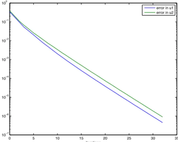
4.1 Belousov-Zhabotinsky Equations
The Belousov-Zhabotinsky equations model non-equilibrium thermodynam-ics, resulting in the establishment of a nonlinear chemical oscillator, see [9], page 322 for details. They are given by
∂tu1−12∂xxu1− u1(1 − u1− ru2) = 0,
∂tu2−12∂xxv + bu1u2= 0. (9)
The hypotheses of Theorem 1 are satisfied for this system after performing the change of variables ˜u1 = 1 − u1, ˜u2 = u2, under the condition that the
components u1 and u2 remain positive. This condition holds, provided that
the initial conditions satisfy u1(x, 0) = u1,0(x) ≥ 0 and u2(x, 0) = u2,0(x) ≥ 0.
Figure 2 shows the linear convergence predicted by the convergence bound of Theorem 1. 0 5 10 15 20 25 30 35 10−7 10−6 10−5 10−4 10−3 10−2 10−1 100 iterations error in u1 error in u2
Fig. 2. Convergence history for the Belousov-Zhabotinsky equations
4.2 FitzHugh-Nagumo Equations The system of reaction diffusion equations
∂tu1−12∂xxu1− f(u1) + u2= 0,
∂tu2−12∂xxu2− u1+ u2= 0,
with f(u1) = u1− u31is called the FitzHugh-Nagumo equations, and describes
how an action potential travels through a nerve. It is the prototype of an excitable system (e.g., a neuron) or an activator-inhibitor system: close to the ground state, one component stimulates the production of both components, while the other one inhibits their growth, see [9], page 161 for details. This system does not satisfy the hypotheses of Theorem 1, but nevertheless we observe linear convergence, as shown in Figure 3.
0 5 10 15 20 25 30 10−7 10−6 10−5 10−4 10−3 10−2 10−1 100 iterations error in u1 error in u2
Fig. 3. Convergence history for the FitzHugh-Nagumo equations
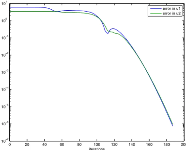
4.3 Lotka-Volterra Equations
The Lotka-Volterra equations with migration term are ∂tu1−252∂xxu1− u1(1 − u2) = 0,
∂tu2−252∂xxu2+ u2(1 − u1) = 0,
and they describe a biological predator-prey system, where both predator and prey are migrating randomly. This system does not satisfy the hypotheses of Theorem 1, and now we observe quite a different convergence behavior, as shown in Figure 4. 0 20 40 60 80 100 120 140 160 180 200 10−7 10−6 10−5 10−4 10−3 10−2 10−1 100 101 iterations error in u1 error in u2
8 St´ephane Descombes, Victorita Dolean and Martin J. Gander
5 Conclusions
Schwarz waveform relaxation algorithms often exhibit superlinear conver-gence, as observed in the last example, see for example [2]. A corresponding convergence analysis requires however quite different techniques from the ones we have presented here, and will appear in an upcoming paper.
References
[1] Martin J. Gander. Overlapping Schwarz waveform relaxation for parabolic problems. In J. Mandel, C. Farhat, and X.-C. Cai, edi-tors, Tenth International Conference on Domain Decomposition Methods. AMS, Contemporary Mathematics 218, 1998.
[2] Martin J. Gander. A waveform relaxation algorithm with overlapping splitting for reaction diffusion equations. Numerical Linear Algebra with Applications, 6:125–145, 1998.
[3] Martin J. Gander, Laurence Halpern, and Fr´ed´eric Nataf. Optimal con-vergence for overlapping and non-overlapping Schwarz waveform relax-ation. In C-H. Lai, P. Bjørstad, M. Cross, and O. Widlund, editors, Eleventh international Conference of Domain Decomposition Methods. ddm.org, 1999.
[4] Martin J. Gander, Laurence Halpern, and Fr´ed´eric Nataf. Optimal Schwarz waveform relaxation for the one dimensional wave equation. SIAM Journal of Numerical Analysis, 41(5):1643–1681, 2003.
[5] Martin J. Gander and Christian Rohde. Overlapping Schwarz waveform relaxation for convection dominated nonlinear conservation laws. SIAM J. Sci. Comp., 27(2):415–439, 2005.
[6] Martin J. Gander and Andrew M. Stuart. Space time continuous analysis of waveform relaxation for the heat equation. SIAM J. Sci. Comp., 19: 2014–2031, 1998.
[7] Eldar Giladi and Herbert B. Keller. Space time domain decomposition for parabolic problems. Numerische Mathematik, 93(2):279–313, 2002. [8] Daniel Henry. Geometric theory of semilinear parabolic equations, volume
840 of Lecture Notes in Mathematics. Springer-Verlag, Berlin, 1981. ISBN 3-540-10557-3.
[9] J. D. Murray. Mathematical biology, volume 19 of Biomathematics. Springer-Verlag, Berlin, 1989. ISBN 3-540-19460-6.
[10] C. V. Pao. Nonlinear parabolic and elliptic equations. Plenum Press, New York, 1992. ISBN 0-306-44343-0.
[11] Aizik I. Volpert, Vitaly A. Volpert, and Vladimir A. Volpert. Traveling wave solutions of parabolic systems, volume 140 of Translations of Math-ematical Monographs. American MathMath-ematical Society, Providence, RI, 1994. ISBN 0-8218-4609-4. Translated from the Russian manuscript by James F. Heyda.