HAL Id: hal-00322191
https://hal.archives-ouvertes.fr/hal-00322191
Submitted on 16 Sep 2008HAL is a multi-disciplinary open access archive for the deposit and dissemination of sci-entific research documents, whether they are pub-lished or not. The documents may come from teaching and research institutions in France or abroad, or from public or private research centers.
L’archive ouverte pluridisciplinaire HAL, est destinée au dépôt et à la diffusion de documents scientifiques de niveau recherche, publiés ou non, émanant des établissements d’enseignement et de recherche français ou étrangers, des laboratoires publics ou privés.
A probabilistic model to predict the formation and
propagation of crack networks in thermal fatigue
Nicolas Malesys, Ludovic Vincent, François Hild
To cite this version:
Nicolas Malesys, Ludovic Vincent, François Hild. A probabilistic model to predict the formation and propagation of crack networks in thermal fatigue. International Journal of Fatigue, Elsevier, 2009, 31 (3), pp.565-574. �10.1016/j.ijfatigue.2008.03.026�. �hal-00322191�
A probabilistic model to predict the formation
and propagation of crack networks in thermal
fatigue
Nicolas Mal´esys,
a,bLudovic Vincent,
aFran¸cois Hild
baCEA Saclay, DEN-DANS/DMN/SRMA/LC2M,
F-91191 Gif sur Yvette cedex, France
b
LMT-Cachan, ENS de Cachan, CNRS UMR 8535, Universit´e Paris 6, 61 avenue du Pr´esident Wilson, F-94235 Cachan cedex, France
Abstract
A probabilistic model is presented to predict the formation and propagation of crack networks in thermal fatigue. It is based on a random distribution of sites where cracks initiate and on the shielding phenomenon corresponding to the re-laxed stress field created around cracks. Currently, the model considers only het-erogeneous uniaxial stress loading even if thermal fatigue is multiaxial. However, the first simulations on a uniaxial mechanical loading representative of the stress gradient that appears in thermal fatigue shocks are in qualitative agreement with experimental results. The larger the stress amplitude, the denser the crack network and the smaller the crack sizes.
1 Introduction
Thermal fatigue is still a major issue in many industrial activities, as proven by very recent publications on this subject in aircraft [1,2], automotive [3,4], metal forming [5–7], braking [8–10], electronic [11,12] and nuclear [13–16] industries. In the case of cooling systems in nuclear power plants, observations revealed the presence of thermal crazing on the internal part of pipes [17]. These crack networks are not a major issue for the structure as long as cracks do not traverse the pipe thickness. Consequently, it is important to know how the crack networks are created and propagate.
The present approach models these phenomena in a probabilistic way, namely the sites where cracks may initiate are described by a Poisson point process. This hypothesis was already used to analyze probabilistic features associated with brittle fracture [18], multiple cracking of composites [19], dynamic frag-mentation of ceramics [20], damage and fracture in cyclic fatigue [21–23]. In many instances, Monte-Carlo simulations are then devised to account for the afore-mentioned phenomena [19,21,24,22]. In the present case, closed form ex-pressions are derived. The conditions for initiation or propagation of cracks are controlled by the probability of finding these sites in the relaxed stress zone created by the cracks already present on the material surface. It is shown that this shielding phenomenon it the key for understanding the partition between stopped and propagating cracks. The present model gives access to various quantities such as the shielding probability, the propagating and formed crack densities. The first quantity gives an information on the possible saturation of the crack network, the second one describes the number of active cracks per unit surface in the network and the last one represents the total number
per unit surface of cracks and is thus directly comparable with the densi-ties of crack networks obtained in thermal fatigue experiments (e.g., SPLASH tests [25]).
The SPLASH configuration, derived from Marsh’s experiments [26], mimics in laboratory environments the conditions for initiation and development of crack networks due to thermal fatigue in the same way as those observed in the mixing zone of cooling systems of Pressurized Water Reactors (PWR). Other experimental facilities have been developed to produce thermal fatigue on tubular specimens (for instance Cythia [27], Biax [28] and Fat3D [29] at the Atomic Research Center (CEA), or Intherpol [30] at ´Electrict´e de France (EDF)). On some of the previous experimental configurations (namely, Biax and Intherpol), a mean axial stress may be superimposed to the cyclic thermal fatigue loading. The advantage of the SPLASH experiment compared with the other ones is its higher frequency that allows for running tests up to one million cycles. The thermal loading is however more difficult to control. A few large scale thermohydraulic tests have been designed to reproduce the mixing conditions in a tee, but the temperature measurements on the surface of the pipe is difficult to perform and the interpretation of such tests requires extensive care.
In the first part of the paper, the framework of the study is presented. Details are given on the formation and propagation of crack networks in thermal fa-tigue by considering several scales of propagation and by introducing various hypotheses on which the probabilistic model is derived. Second, the applied loading is evaluated and the material parameters are identified. In the last part, the results of calculations associated with the probabilistic model are presented and commented. In particular, the changes of the obscuration
prob-ability, the mesocrack density and the propagation density with the number of cycles for a loading representative of SPLASH conditions are obtained. A sim-plified approach of this model is presented by considering a particular crack propagation law. This approach makes it possible to give bounds to all quanti-ties of the probabilistic model. The first results are then compared with those for more severe conditions in order to validate the model in a qualitative way.
2 Crack Networks
2.1 Different Scales
In high cycle fatigue, three scales are considered [31], namely, the micro-, meso-and macroscales. The microscale corresponds to stage I propagation of cracks in high cycle fatigue and interacts with the material microstructure (e.g., the characteristic length is that of grains for the 304L stainless steel considered herein). During this step, the cracks are considered as microstructurally short (they will be referred to as microcracks). This scale ends when the crack prop-agation is no longer dependent on the microstructure, which corresponds to the mesoscale or stage II. Mesocracks are formed after microcrack propaga-tion or alternatively, mesocracks are formed on randomly distributed sites and with an initial size a0 = 64 µm greater than the average grain size of, say,
304L stainless steel (φg = 50 µm). Hence, with such a definition, it is
con-sidered that once a mesocrack has formed, it cannot stop on microstructural obstacles such as grain boundaries (contrary to microcracks). We assume that mesocracks propagate according to a Paris’ law. The last step is concerned with coalesced mesocracks that form a macrocrack (i.e., a long crack).
In the present work, we only deal with crack networks formed at the mesoscale (i.e., made of mesocracks) and not crack networks that may appear at the microscale. Coalescence is not described.
2.2 Crack Obscuration Process
With these three scales, one needs to model how a mesocrack may form from a microcrack and therefore to model interactions of microcracks with other mesocracks. Considering the stress field around a crack, a stress relaxation zone is observed. In this work, this zone is called obscuration (or shielding) zone. If a microcrack belongs to any of these zones, the stress applied to the microcrack is less than the remote stress, thus the microcrack cannot form a mesocrack. Conversely, if the microcrack is not located in a shielding zone, it forms a mesocrack. Similarly, if a mesocrack falls within the obscuration zone of another mesocrack, it will not be able to further propagate. This phenomenon is called obscuration process. In the present case, this process is binary (i.e., a crack is either completely shielded, or not).
2.3 Continuous Formation
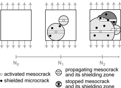
An assumption of continuous formation of cracks is made, namely, the mi-crocracks form mesocracks during the course of time but not all at the same time (in the present case, time is equivalent to number of cycles for a constant amplitude and frequency test). Figure 1 shows the development of cracks in a homogeneous tensile stress field. At the beginning (i.e., when the number of cycles N is equal to 0), there are no mesocracks as shown in Figure 1 when
N
0N
1N
2activated mesocrack
shielded microcrack
propagating mesocrack
and its shielding zone
stopped mesocrack
and its shielding zone
Fig. 1. Depiction of an obscuration process.
N < N0. When the number of cycles increases, microcracks are gradually
created and they eventually form mesocracks with their corresponding obscu-ration zone. Consequently, some microcracks that belong to shielding zones do not form new mesocracks. There are also mesocracks that fall into other shield-ing zones and do not continue to grow (they are stopped). In Figure 1 when N = N1, there are two propagating mesocracks with their respective
obscura-tion zone and three shielded microcracks in the shielding zone of the biggest propagating mesocrack. When N = N2, the smallest propagating mesocrack
of the second step (N = N1) is now in the shielding zone of the biggest one;
it cannot keep on propagating and thus stops. Moreover, a new propagating mesocrack appeared and, in the present case, six microcracks are shielded. If the number of cycles keeps on increasing and if there is only one active crack left (i.e., the largest one), at one stage all the field will be obscured. The weakest link hypothesis [32] then applies, and a Weibull model [33] may be retrieved.
2.4 Microcrack Density
The microstructure of the material is modeled in terms of sites where cracks may be initiated. These sites are approximated by a Poisson point process of intensity λt (i.e., their average number per unit surface or length). A power
law is chosen which leads to a Poisson-Weibull model [19,18]
λt(∆σ) = λ0
µ∆σ
σ0
¶m
(1)
where m is the Weibull modulus (i.e., it characterizes the scatter in local fatigue limits or similarly in local yield stress levels), ∆σ the applied stress variation, and ∆σ0 the scale parameter relative to a reference density λ0 [33].
The considered distribution accounts for microplastic activity close to the ma-terial surface [25]. For this type of mechanism, it was shown that the power law (1) is able to model not only the fatigue properties but also dissipa-tion phenomena [23]. As explained in Secdissipa-tion 2.3, continuous formadissipa-tion of mesocracks corresponds to an incubation “time” (or number of cycles), that is the time needed by microcracks to initiate and propagate before forming a mesocrack. Moreover, one is only interested in the formation and propaga-tion of mesocracks in order to characterize the crack network. Therefore, an additional parameter is introduced in the formulation of the intensity of the Poisson point process that allows one to limit the intensity of the process to mesocracks.
Let λtI be associated with λt but dependent upon the stress variation ∆σ and
the number of cycles N
where ∆σu(N ) corresponds to an incubation stress related to the incubation
time (see Section 3.2) and where h.i Macauley’s brackets. Equation (2) shows that the formation process needs a minimum number of cycles Nmin (i.e., an
incubation time) to form the first mesocrack such that
∆σ − ∆σu(Nmin) = 0. (3)
The continuous formation assumption returns the stress variation ∆σ as a parameter and the number of cycles N as a variable.
2.5 Horizon
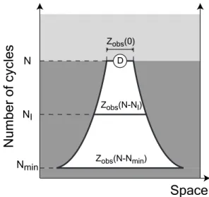
To understand the interaction between existing mesocracks and microcracks, the horizon [20] is the key element. It describes the change of the size of obscuration zones of mesocracks in the space versus number of cycles (Fig-ure 2). Lets us consider a microcrack D that may form a mesocrack after N cycles. For each number of cycles NI (with Nmin < NI < N ), for all the
pos-sible positions of mesocracks, some of them, namely the closest to D, obscure the microcrack location D. This obscured space corresponds to the horizontal bold line in Figure 2 and its size is equal to the size of the obscuration zone Zobs(N −NI), where N −NI correspond to the number of cycles of propagation
of a mesocrack formed at NI cycles and observed after N cycles. The horizon
is the union of all mesocrack positions that obscure D and corresponds to the white zone in Figure 2. Consequently, for a mesocrack to be formed, its horizon should not contain any mesocrack. In the present setting, obscuration occurs at the mesoscopic level because a microcrack shields neither a microcrack nor a mesocrack, and because only the propagation of mesocracks is taken into
account in the formation of crack networks. Number of cycles Space N D NI Zobs(N-NI) Zobs(N-Nmin) Zobs(0) Nmin
Fig. 2. Horizon of a given site location D.
2.6 Obscuration Probability
Apart from shielding effects, the probability of finding Nµ = ν mesocracks
within a uniformly loaded examination domain Ω is expressed in terms of a Poisson distribution
P (Nµ= ν, Ω) =
[λtI(∆σ, N ) Z]ν
ν! exp [−λtI(∆σ, N ) Z] (4)
where Z is the size of the domain Ω so the product λtI(∆σ, N ) Z corresponds
to the average number of mesocracks in a domain Ω loaded for N cycles with a stress variation ∆σ, when shielding effects are not considered. The presence of one or more mesocracks in the horizon of a microcrack or a mesocrack induces its obscuration. Hence, one introduces the obscuration probability Pobs that corresponds to the probability of finding one or more mesocracks in
this horizon Pobs(∆σ, N ) = 1 − exp h −λtI(∆σ, N ) ˆZobs(∆σ, N ) i (5)
where ˆZobs(∆σ, N ) is the measure of the horizon also called the mean
obscu-ration zone [20] ˆ Zobs(∆σ, N ) λtI(∆σ, N ) = N Z Nmin Zobs(∆σ, N − NI) dλtI dNI (∆σ, NI) dNI.(6)
Pobs characterizes the degree of damage (i.e., the fraction of obscured zones)
of the network. By analyzing its value, the state of cracking in the network can be assessed.
2.7 Mesocrack Density
The density of activated mesocracks (i.e., the propagating and stopped mesoc-racks taking into account shielding effects) is calculated from the formation density λtI and the obscuration probability Pobs. This density, denoted by λm,
corresponds to the density of microcracks that meet all the conditions to form a mesocrack, namely, a number of cycle N greater than the incubation time and the absence of a shielding zone around its location (i.e., this microcrack is not obscured by any mesocrack). The increment of mesocrack density λm is
related to that of λtI by
dλm
dN (∆σ, N ) = dλtI
dN (∆σ, N ) × [1 − Pobs(∆σ, N )] . (7) The mesocracks that are not obscured by other mesocracks correspond to the active (i.e., propagating) mesocracks. Let λmP denote the propagation density
λmP (∆σ, N ) = λm(∆σ, N ) × [1 − Pobs(∆σ, N )] . (8)
The formed mesocrack density λm may be compared to observations during
inspections of zones where, say, thermal crazing is suspected to occur. How-ever, the most crucial information is the active mesocrack density λmP that
is critical for the life of a component. This quantity can be estimated only by comparing two different states of cracking. The presented model is now applied to analyze experiments on a 304L austenitic stainless steel.
3 Material and Loading Parameters
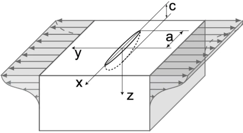
This work considers only one direction for mesocrack formation and propa-gation on the surface of the material and a propapropa-gation in the depth along a direction perpendicular to the surface. A set of semi-elliptical cracks of length 2a and depth c is considered, with a = c = 67 µm at crack formation. It is assumed that the shape of the crack remains semi-elliptical, even though the aspect ratio c/a may change with the number of cycles since the propa-gation on the surface depends on the stress profile σyy along the z direction
(Figure 3).
✁
✂
✄
☎
3.1 Weibull Parameters
With a weakest link hypothesis and a power law used to described the microc-rack density, a two-parameters Weibull law is retrieved to describe the failure probability for a sample uniformly loaded in the endurance regime (i.e., when N → +∞)
PF = P (Nµ ≥ 1, Ω) = 1 − P (Nµ= 0, Ω) = 1 − exp (−λtZ) (9)
The Weibull parameters may therefore be determined by analyzing endurance data for which the majority of the number of cycles is used in the formation of a mesocrack. An evaluation of the endurance limit of 304L used in the present study has been obtained by following the staircase method [34]. This method, originally proposed by Dixon and Mood [35], gives access to an estimate of the average value σ∞ and the standard deviation σ∞ of the endurance limit.
These two quantities are expressed according to the Weibull model as
σ∞= σ0 (λ0Zef f) 1/mΓ µ 1 m + 1 ¶ (10) and σ∞= σ0 (λ0Zef f) 1/m s Γ µ2 m + 1 ¶ − Γ2 µ1 m + 1 ¶ (11)
where Zef f is the measure of the effective surface, and Γ the gamma function
defined by Γ (p) = +∞ Z 0 tp−1exp (−t) dt. (12)
Knowing the experimental values of the average and the standard deviation of the fatigue limit distribution, it is possible to determine the Weibull modulus m with the following equation
à σ∞ σ∞ !2 = Γ ³2 m + 1 ´ Γ2³1 m + 1 ´ − 1 (13)
and then any of the two equations (10) or (11) is used to determine the value of the last undetermined parameter, namely the scale parameter λ0/σm0 . In
this study, m = 20 and σ0 = 451 MPa for a value of λ0 arbitrarily set to
1 crack/mm2
.
This analysis shows one of the benefits of the unified framework introduced herein. In the present section, a weakest link hypothesis was made in conjunc-tion with the use of a Poisson point process. A Weibull model is then retrieved, and the parameters of the intensity of the Poisson point process are identical to classical Weibull parameters. Furthermore, the identified parameters will be used later on in a situation in which the weakest link hypothesis does not necessarily apply.
3.2 Incubation Stress
As mentioned in the previous part, microcracks may form mesocracks only after a certain number of cycles also called “incubation time.” The connection between this incubation time and the formation density is obtained with the incubation stress ∆σu(N ) [Equation (2)]. The difference between the stress
fatigue limit ∆σ∞
∆σ∞= ∆σ − ∆σu(N ) . (14)
To obtain a random number of cycles for mesocrack formation, one only needs to consider the Poisson point process whose intensity is directly related with the previous relationship, via Equation (2). Hence, for a constant mesoscopic stress variation, and a given number of cycles N , a direct use of the Poisson point process gives access to the probability of finding Nµ formed mesocracks
in the considered zone. Conversely, for a constant mesoscopic stress varia-tion, considering all possible probabilities of finding Nµ formed mesocracks
in the considered zone (i.e., from 0 to 1), a distribution of the number of cycles to crack formation is retrieved. In uniaxial fatigue tests on a homoge-neously loaded specimen, the difference between the number of cycles to form a mesocrack NI and the number of cycles to failure NF of the specimen is a
small proportion of this last value, namely
NF − NI
Nf ≪ 1
(15)
In this particular case, considering Equation (14) and a Poisson point process of intensity given by Equation (2), one obtains for a constant mesoscopic stress variation:
• a failure probability for a given number of cycles N (i.e., the probability of finding at least one mesocrack in the considered zone).
• a distribution of the number of cycles to failure of the specimen (i.e., the distribution of the number of cycles for a probability of finding at least one mesocrack ranging from zero to unity).
The W¨ohler curves give access to the variation of stress versus the number of cycles to failure with a given failure probability. The probability curve PF = 0.5 has been estimated, for 304L stainless steal, by considering the
half-life stress variation measured in strain-controlled fatigue tests versus the number of cycles N25 (i.e., number of cycles for which a 25% decrease of
maximum stress is obtained). These tests were performed at 165◦
C and with ˙ε = 2 × 10⁻³
s−1
[36,37].
Considering a Poisson point process, such a probability curve corresponds to a constant value of its intensity [Equation (2)], and thus to a constant value of ∆σ∞ [Equation (14)]. Therefore, the incubation stress variation ∆σu(N )
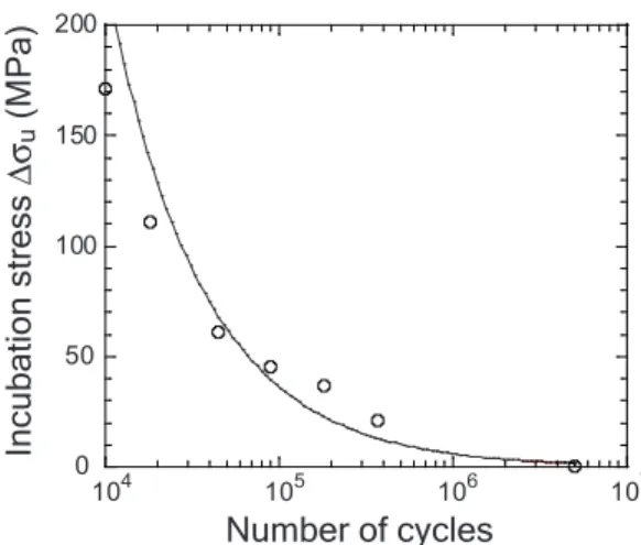
may be modeled, say, by a power law [Equation (16)], identified on the change of the difference between the stress variation and the average endurance limit (multiplied by two), versus the number of cycles to failure (Figure 4)
∆σu(N ) = σdN−1/η (16)
where σd and η are material parameters (σd = 3.1 × 10⁵ MPa and η = 1.3 for
the considered material). The average endurance limit is estimated for 5 × 10⁶
cycles with staircase stress-controlled fatigue tests. With this power law, it is assumed that ∆σu(N → +∞) → 0, which is consistent with the previous
analysis. Therefore, the model describes the high cycle fatigue domain (i.e., when 104
< N < +∞) and the endurance domain (i.e., when N → +∞) in the same framework.
0 50 100 150 200 Incu bati on st res s ∆σ u (MP a) Number of cycles 105 104 106 107
Fig. 4. Identification of the incubation stress ∆σu as a function of the number of
cycles. The open symbols correspond to half-life stress variations measured
dur-ing strain-controlled tests performed on 304L stainless steel at 165◦
C, and with ˙ε = 2 × 10⁻³ s−1 [36,37]. The solid line is a power-law fit by least squares
minimiza-tion.
3.3 Loading Condition
In this study, crack networks are due to thermal fatigue and the loading con-ditions are identified for the SPLASH configuration [25]. The test consists in heating in a continuous way by Joule effect a specimen and to sprinkle distilled water in a cyclic way onto two opposite faces of the specimen. The temperature variation on the surface of the specimen is about 150◦
C and the duration of sprinkling is 0.25 s each 7.75 s. Maillot [25] carried out thermo-elastoplastic finite element calculations to determine the mechanical loading associated with the recorded temperature history. The loading is almost equib-iaxial and the variation of stress from the coldest instant (T = Tmin) to the
hottest one (T = Tmax) is estimated at every point of the structure. A 3rd
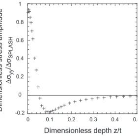
degree polynomial is identified on the calculated stress profile (Figure 5) to model the depth dependence for z/t ≤ 0.16 of the normal stress
∆σyy ∆σSP LASH = −529.8 µz t ¶3 + 218.3 µz t ¶2 −28.3 µz t ¶ + 1 (17) where ∆σSP LASH = 370 MPa and t is the specimen thickness.
-0.2 0 0.2 0.4 0.6 1 0 0.1 0.2 0.3 0.4 0.5 Dimensionless depth z/t Dime nsio nless stre ss am plitud e ∆σ yy /∆σ SPLASH 0.8
Fig. 5. Computed stress profile.
3.4 Propagation Law
Crack networks obtained with the previous stress profile are mainly superficial so the aspect ratio c/a of cracks, which represents the crack shape, is often small (i.e., less than 0.2). The propagation of this type of cracks was studied by Wang and Lambert [38]. It is based on the use of weight functions determined from finite element results and gives the stress intensity factors ∆KIA and
∆KIC associated with semi-elliptical cracks [Figure 6(a)]. A Paris’ law is then
applied to calculate the crack sizes a and c
da dN = C (∆KIA) p and dc dN = C (∆KIC) p (18) where C = 3.74 × 10⁻¹⁰ mm/MPa√m)−n and p = 4.04 identified at 320◦ C for the 304L stainless steel considered in this study. Only slight modifications of
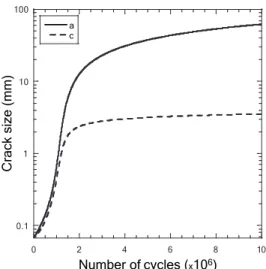
these values are obtained for crack propagation tests performed at room tem-perature [38] and therefore, these parameters are considered constant during a complete thermal cycle. When the number of cycles is small (i.e., at the beginning of the load history), the crack is propagating on the surface and in-depth [Figure 6(b)]. Yet, as soon as the latter reaches a depth such that the loading becomes compressive, the crack growth rate decreases. The initial conditions for the crack shape are a = c = 67 µm (i.e., semi circular). Upon loading, the crack shape remains almost circular during one million cycles, then tends quickly towards an elliptic shape during the next million cycles [Figure 6(c)].
3.5 Obscuration Zone
By studying the stress field around a penny-crack shaped on a plane submitted to a unidirectional tensile field perpendicular to its propagation direction, a stress relaxation appears around the crack [39,40]
Zobs(N ) = S [ka (N )]n (19)
where S = 2 and k = 1.334 for a space of dimension n = 1 [41], and S = π and k = 1.428 for n = 2 [42]. In the present case, the cracks are initiating only on the surface, thus the obscuration is considered only on the surface but one must take into account the effect of mesocrack depth on Zobs. A first
approximation is made on this quantity. It is considered that it is equal to the surface of the crack (i.e., the surface of a semi-ellipse of major axis equal to a and minor axis equal to c)
Stre ss in tensit y fa c to r (MP a.m 1/2 ) 2 4 6 8 10 12 14 0,1 1 10 K IA vs a K IC vs c Length a and c (mm)
(a) Stress intensity factors vs. crack length 0.1 1 10 100 0 2 4 6 8 10 a c Number of cycles (x106) Crack size (mm)
(b) Crack sizes vs. number of cycles
0 0.2 0.4 0.6 0.8 1 0 2 4 6 8 10 Number of cycles (x106) Ellipti cit y r ati o c/ a
(c) Aspect ratio vs. number of cycles
Fig. 6. Crack propagation features for a SPLASH loading.
The deeper the crack, the larger the obscuration zone on the surface of the specimen.
4 Results
In this section, the results of the probabilistic model are presented and com-pared with results obtained for a more severe loading condition. Some bounds
are also introduced in order to get analytical expression of the model quanti-ties.
4.1 SPLASH Conditions
The SPLASH conditions, presented in Section 3.3, are considered. The first result of this loading condition is the propagation of the first mesocrack de-scribed in Section 3.4. These results are regarded as parameters of the proba-bilistic model, necessary for the calculation of the obscuration probability, the formed and propagating mesocrack densities.
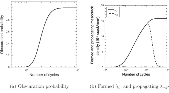
The change of the obscuration probability Pobs [Equation (5)] with the number
of cycles is given in Figure 7(a). Figure 7(b) shows the corresponding changes of the formed and propagating mesocrack densities λm and λmP. At the
be-ginning, the obscuration probability is equal to zero because of the absence of mesocracks in the sample and thus no obscuration occurs. Both densities are also equal to zero. As soon as the number of cycles reaches the minimum num-ber of cycles (i.e., N = Nmin), when a microcrack forms the first mesocrack,
the three quantities begin to increase. When the first mesocrack is formed, an obscuration zone appears in its vicinity and the obscuration probability, which is an increasing function of the size of the obscuration zone, increases. From this moment on, new mesocracks will continue to form with the creation of new obscuration zones and previously formed mesocracks will grow, induc-ing a growth of their associated obscuration zone. This phenomenon is also accompanied by the arrest of mesocracks that fall into the obscuration zone of other mesocracks and by the impossibility of some microcracks to form new mesocracks because of the relaxation stress field in their vicinity.
First, the number of arrested mesocracks is less than the number of formed mesocracks, which is confirmed by the increase of the propagating mesocrack density. The increment of arrested mesocracks compared with the increment of new mesocracks is justified by the increasing difference between the two densi-ties [Figure 7(b)]. The maximum of the propagating crack density corresponds to the number of cycles for which the increment of arrested mesocracks be-comes greater than that of newly formed mesocracks. From this moment on, the propagating crack density decreases and tends to zero, the obscuration probability tends to 1 (i.e., the studied domain becomes more and more ob-scured) and the mesocrack density saturates.
0 0.2 0.4 0.6 0.8 1 106 107 Number of cycles Obscurati on pr obab ility
(a) Obscuration probability
✁ ✂✄ ✂☎✁ ✆✝ ✂✞✠✟ ✂✞☛✡ ✂✞☛☞ ✂✄☛✌ ✍✏✎ ✍✎✒✑ ✓✕✔✗✖✙✘✛✚✢✜✤✣✦✥✛✧✩★✪✧✦✫✚✭✬ ✮✯ ✰✱ ✲ ✳✴ ✵ ✳✶ ✰✯ ✶ ✴ ✷ ✴ ✸ ✹ ✵ ✷ ✱ ✲✺ ✯ ✻ ✰ ✴ ✻ ✼ ✳ ✲ ✵✺ ✹ ✸✽ ✾ ✿ ❀❁ ❂ ✻ ✰ ✴ ✻ ✼ ❃✱ ✱ ❄❅
(b) Formed λm and propagating λmP
mesocrack densities
Fig. 7. Results of the probabilistic model for a SPLASH loading.
Let us point out that the obscuration probability, the mesocrack and prop-agating crack densities are related to the surface of the specimen because of the nature of thermal crazing. However, the propagation itself accounts for the in-depth variation of the stress field (see Section 3.3).
4.2 Bounds
Let us derive bounds for the model. An upper bound to the obscuration prob-ability, and lower bounds to the mesocrack and propagating crack densities are given. Let us assume that the crack depth c is equal to a maximum value cmax. From Figure 6(a), if one adopts a threshold value for the stress
inten-sity factor ∆Kth under which the mesocrack is not propagating any more, the
maximum crack depth value cmax reads
cmax= c (∆KI = ∆Kth) . (21)
At the same time, ∆KIA is almost constant for any value of a. This case
corresponds to the propagation of a channeling crack [43], i.e., the surface crack propagation velocity d˜a/dN is constant
d˜a
dN = C (∆KIAmax)
p
= C∆Kmaxp (22)
where C and p are parameters of the Paris’ law. With these assumptions, the half crack size ˜a becomes
˜
a = ainit+ C∆Kmaxp × (N − NI) (23)
where ainit is the initial size of the mesocrack (here, ainit = 67 µm) and the
obscuration probability ˜Pobs reads
lnh1 − ˜Pobs(N )
i
= I1+ I2 (24)
with
and I2 = −πcmaxC∆Kmaxp mλ0 µ∆σ σ0 ¶m × µ σ d ∆σ ¶η B σdN −1/η I ∆σ , 1 − η, m NI=N NI=Nmin (26) where B is the function defined by
B (x, a, b) =
x
Z
0
ta−1(1 − t)b−1dt. (27)
A lower bound to the formed mesocrack density ˜λm is obtained by using
Equation (7) in which Pobs is replaced by ˜Pobs. Similarly, a lower bound to
the propagating mesocrack density ˜λmP is obtained by using Equation (8).
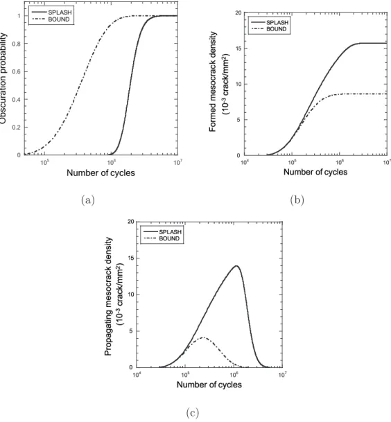
The results presented in Figure 8 are obtained with a maximum crack depth cmax equal to 3.5 mm and they prove that for a mesocrack size always equal
to its maximum value, the studied domain is obscured faster than in the case of a normal propagation of mesocracks. The formed mesocrack density increases in the same way as the reference density but slows down earlier and saturates at a lower value. For small numbers of cycles (i.e., N < 105
), the propagating crack density and its bound evolve in the same way but the latter reaches more quickly its maximum value (after 4 × 10⁵
cycles) whereas the normal propagating crack density needs approximatively 106
cycles to reach its ultimate level.
4.3 Comparison with a More Severe Loading
The previous results were presented in the case of SPLASH conditions. In other cases, such as Fast Breeder Reactors (FBR), the temperature on the
in-0 0.2 0.4 0.6 0.8 1 105 106 107 SPLASH BOUND Number of cycles Obscur ation pr obabilit y (a) ✁ ✂✄ ✂☎✁ ✆✝ ✂✄✟✞ ✂✠☛✡ ✂✄☛☞ ✂✠☛✌ ✍✏✎✒✑✔✓✕✍✏✖ ✗✙✘✛✚✒✜✕✢ ✣✥✤✧✦✩★✫✪✭✬✯✮✱✰✱✲✒✳✱✲✱✴✪✛✵ ✶✷ ✸✹ ✺ ✻ ✹ ✺✼ ✷ ✽ ✸✾ ✽ ✿ ✻ ✺❀ ✼ ❁ ❂❃ ❄ ❅ ❆❇ ❈ ✽ ✸✾ ✽ ✿ ❉✹ ✹ ❊❋ (b) ✂✁☎✄ ✂✁☎✆ ✂✁✞✝ ✂✁✞✟ ✠☛✡✌☞✎✍✏✠✏✑ ✒✔✓✖✕✌✗✙✘ ✚✜✛✣✢✥✤✧✦✩★✫✪✭✬✧✮✙✯✰✮✭✱✦✖✲ ✁ ✳ ✎✁ ✴✳ ✵✶✁ ✷✸✹ ✺✻ ✼✻ ✽ ✾✿ ✼ ❀❁ ❂ ✹ ❃✸ ✻ ❃ ❄❅ ❁ ✿ ❂ ✾ ✽❆ ❇ ❈ ❉❊ ❋ ❃✸ ✻ ❃ ❄ ● ❀ ❀ ❍■ (c)
Fig. 8. Comparison between the model quantities and their respective bounds
(cmax = 3.5 mm and KIA= 13.5 MPa√m).
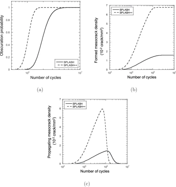
ternal surface of the pipe is higher as well as temperature gradients under the surface. Therefore the stress levels may be larger. In this part, one proposes to apply the model to the case of a higher load level. The associated model is based on Equation (17) where ∆σSP LASH is replaced by ∆σSP LASH++ with
∆σSP LASH++ > ∆σSP LASH. The obscuration probability tends to 1 faster in
the case of a higher load level [Figure 9(a)]. Moreover, the formed mesoc-rack density [Figure 9(b)] has higher values compared with those obtained in the SPLASH loading conditions, and its saturation is faster. The
propa-0 0.2 0.4 0.6 0.8 1 106 107 SPLASH SPLASH++ Number of cycles Obscu rat ion pro bability (a) ✁ ✂ ✄ ☎ ✆ ✝ ✁✟✡✠ ✁✟☞☛ ✁✟☞✌ ✁✍☞✎ ✏✒✑✔✓✍✕✖✏✒✗ ✏✒✑✔✓✍✕✖✏✒✗✙✘✚✘ ✛✢✜✤✣✦✥★✧✪✩✬✫★✭✯✮✔✰✱✮★✲✧✴✳ ✵✶ ✷✸ ✹ ✺ ✸ ✹✻ ✶ ✼ ✷✽ ✼ ✾ ✺ ✹✿ ✻ ❀ ❁❂ ❃ ❄ ❅❆ ❇ ✼ ✷✽ ✼ ✾ ❈✸ ✸ ❇❉ (b) ✁ ✂ ✄ ☎ ✆ ✝ ✞ ✁✟✡✠ ✁✟☞☛ ✁✟☞✌ ✁✍☞✎ ✏✒✑✔✓✍✕✒✏✗✖ ✏✒✑✔✓✍✕✒✏✗✖✔✘✙✘ ✚✜✛✣✢✥✤✧✦✩★✫✪✭✬✧✮✰✯✱✮✭✲✦✴✳ ✵✶✷ ✸✹ ✺✹ ✻ ✼✽ ✺ ✾✿ ❀ ✷ ❁✶ ✹ ❁ ❂❃ ✿ ✽ ❀ ✼ ✻❄ ❅ ❆ ❇❈ ❉ ❁✶ ✹ ❁ ❂ ❊ ✾ ✾ ❉❋ (c)
Fig. 9. Comparison between SPLASH loading and a higher loading (SPLASH++).
gating crack density [Figure 9(c)] increases faster and reaches a maximum value greater than in the case of the SPLASH loading conditions. Its decrease also occurs earlier. Therefore, one concludes that the crack network obtained with a higher load level is denser than that obtained in the normal loading conditions, and its saturation is faster.
4.4 Mesocrack Sizes Distribution
The experimental results [25] give access to the crack network density at sev-eral time steps. To obtain the distribution of mesocrack sizes, one should know, at every time, the density of mesocracks that formed at Ni cycles and their
re-spective duration of propagation. The density increment of mesocracks formed during the time increment dNi is given by
dλ∗
m(Ni) =
dλm
dNi
(Ni) dNi. (28)
These mesocracks may be obscured by only larger mesocracks (i.e., mesocracks that were formed before). One associates with λ∗
m the obscuration probability
at N = Ni+ Np of the older mesocracks that formed before Ni on the
mesoc-racks that formed at Ni cycles and that have potentially propagated for Np
cycles lnh1 − Pobsi,p(Ni, Np) i = − Ni Z Nmin dλtI dNI (NI) Zobs(Np+ Ni− NI) dNI. (29)
Thus, the density of mesocracks formed during the time increment dNi and
that have propagated for Np cycles or less is given by
dλi,ps (Ni, Np) =
dλm
dNi
(Ni) dNi× Pobsi,p(Ni, Np) . (30)
The same type of expression is written for the density of mesocracks formed during the same time increment and that have propagated for Np+ dNp cycles
or less. The difference between these two last quantities will give the increment of density of mesocracks formed during dNi cycles, at N = Ni cycles, and that
Np+ dNp cycles. This density increment is written as dλi,pa (Ni, Np) = ∂λi,p s (Ni, Np) ∂Np dNp (31)
and since λm does not depend on Np
dλi,pa (Ni, Np) = dλm(Ni) dNi × ∂Pobsi,p(Ni, Np) ∂Np dNidNp. (32) ✂✁☎✄✆ ✂✁☎✄✝ ✂✁☎✄✞ ✁ ✂✁ ✟✠✁ ✡☛✁ ☞✍✌✏✎✒✑✓☞✍✔ ☞✍✌✏✎✒✑✓☞✍✔✖✕☛✕ ✗✙✘✓✚✛✓✜✍✢✘✣✜✍✤✙✥✖✦✧✩★✪✘✬✫✮✭✯✭✯✰ ✱✲ ✳✲ ✴✵ ✶ ✷✸ ✹ ✺ ✹✻✼ ✷ ✶✽ ✾ ✿ ✼ ✶ ✾❀ ❀ ✹ ✺ ✳ ✹ ✼ ✾❁❂ ✵ ❁ ❃ ✼ ❄❁❂ ✵ ❁ ❃ ❅ ✳ ✳ ❆❇ (a) ✂✁✄ ☎ ☎✆✁✄ ✝ ✝✞✁✄ ✟ ✠☛✡✌☞✎✍✏✠☛✑ ✠☛✡✌☞✎✍✏✠☛✑✓✒✔✒ ✕✗✖✘✌✙✛✚✢✜✞✣✥✤✧✦✩★✪✙✬✫✮✭✯✭✯✰ ✱✳✲✵✴✶ ✱✳✲✵✴✷ ✱✳✲✵✴✸ ✹✺ ✻✺ ✼✽ ✾✿❀ ❁ ❂ ❁❃❄ ✿ ✾❅ ❆ ❇ ❄ ✾ ❆❈ ❈ ❁ ❂ ✻ ❁ ❄ ❆❉❊ ✽ ❉ ❋ ❄ ●❉❊ ✽ ❉ ❋ ❍ ✻ ✻ ■❏ (b)
Fig. 10. Distribution of crack sizes after 5 million cycles for the SPLASH and SPLASH++ loading conditions.
In Figure 10, the cumulated densities of stopped mesocracks after 5 millions cycles are shown as functions of the respective half crack sizes [Figure 10(a)] and depths [Figure 10(b)] for the SPLASH and SPLASH++ loading condi-tions (in the two cases, after 5 millions cycles, the networks are saturated so the density of stopped mesocracks corresponds to the network density ob-served in the SPLASH test for example). These curves show that there is no crack with a depth greater than 3 mm in the SPLASH case, and 2.5 mm in the SPLASH++ case (corresponding to a constant value of the cumulative density). Moreover, all stopped mesocracks associated with the SPLASH++ loading condition have sizes on the surface less than 10 mm, whereas the
stopped mesocracks associated to the SPLASH condition have sizes around 10-20 mm. These results are in qualitative agreement with the experimental results that show crack networks denser and having smaller crack sizes in the case of a stronger loading.
5 Conclusion
A probabilistic model was introduced to account for mesocrack formation, propagation and arrest. The obscuration probability characterizes the state of damage of the network. The formed mesocrack density can be compared directly with actual experimental observations of crack networks. The propa-gating crack density is the key quantity for evaluating the propagation activity in the network, namely, the part of the crack distribution that might be fatal to a structure. All quantities were studied for the particular case of SPLASH loadings. The results of the model are in good qualitative agreement with experimental observations since they present a saturation of crack networks induced by the very small value of the propagating crack density. The arrest of mesocracks in the depth of the material is also accounted for.
In order to find analytical expressions of the model quantities, bounds were proposed by choosing simple laws for the change of crack sizes (i.e., the crack depth and the half-size crack on the surface). These assumptions made it possible to analytically express the formation and propagation of networks made of cracks whose depths are constant and equal to the maximum values observed in the previous case, and for which the surface propagation velocity is maximum. The resulting crack network is less dense than the SPLASH network and saturates faster. The influence of a more severe load level was
studied and the main conclusion was that the larger the stress variation, the faster the saturation and the denser the crack network with a distribution of smaller crack sizes.
The cases studied herein do not take into account the various possible orien-tations of the formed and propagating mesocracks (see Ref. [25] on SPLASH tests) and, consequently, the shielding conditions between mesocracks of dif-ferent orientations. In order to compare quantitatively the predictions of the model and experimental results, the model is currently generalized, by taking into account all the directions of formation and propagation of mesocracks on the surface, as well as their different possible interactions. Last coalescence needs to be accounted for to fully characterize the crack network.
6 Acknowledgment
This work was partially funded by ´Electricit´e de France R&D. The authors wish to thank Dr. Sa¨ıd Taheri for his support.
References
[1] M. Mansoor, I. Islam and A. Tauqir, Restricted life of after burner manifold assemblies due to stress raisers, Eng. Fail. Analysis 14 (2007) 1280-1285.
[2] L. R´emy, A. Alam, N. Haddar, A. K¨oster and N. Marchal, Growth of small cracks and prediction of lifetime in high-temperature alloys, Mat. Sci. Eng. A 468-470(2007) 40-50.
alloys under superimposed thermal-mechanical fatigue and high-cycle fatigue loading, Mat. Sci. Eng. A 468-470 (2007) 184-192.
[4] V. Firouzdor, M. Rajabi, E. Nejati and F. Khomamizadeh, Effect of microstructural constituents on the thermal fatigue life of A319 aluminum alloy, Mat. Sci. Eng. A 454-455 (2007) 528-535.
[5] C. Li, H. Yu, G. Deng, X. Liu and G. Wang, Numerical Simulation of Temperature Field and Thermal Stress Field of Work Roll During Hot Strip Rolling, J. Iron Steel Res. 14 (2007) 18-21.
[6] W. S. Dai, M. Ma and J. H. Chen, The thermal fatigue behavior and cracking characteristics of hot-rolling material, Mat. Sci. Eng. A 448 (2007) 25-32.
[7] A. Persson, S. Hogmark and J. Bergstrom, Simulation and evaluation of thermal fatigue cracking of hot work tool steels, Int. J. Fat. 26 (2004) 1095-1107.
[8] X. Tong, H. Zhou, Z. Zhang, N. Sun, H. Shan and L. Ren, Effects of surface shape on thermal fatigue resistance of biomimetic non-smooth cast iron, Mat. Sci. Eng. A 467 (2007) 97-103.
[9] G. Degallaix, P. Dufrenoy, J. Wong, P. Wicker and F. Bumbieler, Failure mechanisms of TGV brake discs, Key Eng. Mat. 345-346 (2007) 697-700.
[10]C. H. Gao, J. M. Huang, X. Z. Lin and X. S. Tang, Stress Analysis of Thermal Fatigue Fracture of Brake Disks Based on Thermomechanical Coupling, J. Tribol. 129 (2007) 536-543.
[11]X. W. Liu and W. J. Plumbridge, Damage Produced in Solder Alloys during Thermal Cycling, J. Electronic Mat. 36 [9] (2007) 1111-1120.
[12]R. L. J. M. Ubachs, P. J. G. Schreurs and M. G. D. Geers, Elasto-viscoplastic nonlocal damage modelling of thermal fatigue in anisotropic lead-free solder, Mech. Mat. 39 (2007) 685-701.
[13]S. Taheri, Some advances on understanding of high cycle thermal fatigue crazing, J. Press. Vessel Tech. 129 [3] (2007) 400-410.
[14]O. Ancelet, S. Chapuliot, G. Henaff and S. Marie, Development of a test for the analysis of the harmfulness of a 3D thermal fatigue loading in tubes, Int. J. Fat. 29 (2007) 549-564.
[15]R. Desmorat, A. Kane, M. Seyedi and J.-P. Sermage, Two scale damage model and related numerical issues for thermo-mechanical High Cycle Fatigue, Eur. J. Mech. A/Solids 26 (2007) 909-935.
[16]M. Missirlian, F. Escourbiac, M. Merola, A. Durocher, I. Bobin-Vastra and B. Schedler, Damage evaluation under thermal fatigue of a vertical target full scale component for the ITER divertor, J. Nuclear Mat. 367-370 (2007) 1330-1336.
[17]J.-M. Stephan, F. Curtit, C. Vindeirinho, S. Taheri, M. Akamatsu and C. Peniguel, Evaluation of the risk of damage in mixing zones: EDF R & D programme, Proceedings Fatigue 2002 , 1707-1714.
[18]D. Jeulin, Mod`eles morphologiques de structures al´atoires et changement d’´echelle, (th`ese d’´Etat, University of Caen, 1991).
[19]R. Gulino and S. L. Phoenix, Weibull Strength Statistics for Graphite Fibres Measured from the Break Progression in a Model Graphite/Glass/Epoxy Microcomposite, J. Mater. Sci. 26 [11] (1991) 3107-3118.
[20]C. Denoual, G. Barbier and F. Hild, A Probabilistic Approach for Fragmentation of Ceramics under Impact Loading, C. R. Acad. Sci. Paris 325 [S´erie IIb] (1997) 685-691. See also, C. Denoual and F. Hild, A Damage Model for the Dynamic Fragmentation of Brittle Solids, Comp. Meth. Appl. Mech. Eng. 183 (2000) 247-258.
[21]J. Weiss, Endommagement en viscoplasticit´e cyclique sous chargement multiaxial `a haute temp´erature d’un acier inoxydable aust´enitique, (PhD
dissertation, ´Ecole Nationale Sup´erieure des Mines de Paris, 1992).
[22]B. Fedelich, A stochastic theory for the problem of multiple surface crack coalescence, Int. J. Fract. 91 (1998) 23-45.
[23]C. Doudard, S. Calloch, P. Cugy, A. Galtier and F. Hild, A probabilistic two-scale model for high cycle fatigue life predictions, Fat. Fract. Eng. Mat. Struct. 28(2005) 279-288.
[24]A. Bataille and T. Magnin, Surface damage accumulation in low-cycle fatigue: Physical analysis and numerical modeling, Acta Metall. Mater. 42 [11] (1994) 3817-3825.
[25]V. Maillot, Amor¸cage et propagation de r´eseaux de fissures de fatigue thermique dans un acier inoxydable aust´enitique de type X2 CrNi 18-09 (AISI 304 L), (PhD dissertation, Universit´e des Sciences et Technologie de Lille, 2003).
[26]D. J. Marsh, A thermal shock fatigue study of 304 and 316 stainless steels, Fat. Engng. Mater. Struct. 4 [2] (1981) 179-195.
[27]C. Robertson, M. C. Fivel and A. Fissolo, Dislocation substructure in 316L stainless steel under thermal fatigue up to 650 K, Mat. Sci. Eng. A A315 (2001) 47-57.
[28]C. Robertson and S. Chaise, Bilan des essais de fatigue thermique avec contrainte de traction sur un acier aust´enitique, (CEA Saclay, technical note, DMN/SRMA/LC2M/NT-2004-2690-A 2004).
[29]O. Ancelet, ´Etude de l’amor¸cage et de la propagation des fissures sous chargement thermique cyclique 3D, (PhD dissertation, University of Poitiers, France, 2006).
[30]F. Curtit and J.-M. Stephan, Essais de fatigue thermique sur structures, Proceedings Congr`es national Mecamat 2007 , 246-255.
[31]K. J. Miller, Materials science perspective of metal fatigue resistance, Mat. Sci. Tech. 9 (1993) 453-462.
[32]A. M. Freudenthal, Statistical Approach to Brittle Fracture, in: Fracture, H. Liebowitz, ed., (Academic Press, New York (USA), 1968), 591-619.
[33]W. Weibull, A Statistical Theory of the Strength of Materials, (Roy. Swed. Inst. Eng. Res., Report 151, 1939).
[34]L. Vincent and G. Perez, ´Etude de la fatigue d’un acier inox aux faibles niveaux de chargement. Rapport d’avancement no. 2, (CEA Saclay, technical note, DMN/SRMA/LC2M/NT/2004-2687/A 2004).
[35]W. J. Dixon and A. M. Mood, A method for obtaining and analyzing sensitivity data, J. Am. Statis. Assoc. 43 (1948) 109-126.
[36]M. Mottot and M. Noblecourt, ´Etude du comportement en fatigue oligocyclique `
a 165◦
C et 320◦
C du 304L pour de faibles niveaux de d´eformations (ε ≤ 1%), (CEA Saclay, technical note, DMN/SRMA/NT/2001-2403 2001).
[37]M. Mottot and M. Noblecourt, ´Etude du comportement en fatigue oligocyclique d’aciers de type Z2 CN 18-10 (304L) `a 20◦
C et 300◦
C, (CEA Saclay, technical note, DMN/SRMA/NT/2002-2513 2002).
[38]X. Wang and S. B. Lambert, Stress intensity factors for low aspect ratio semi-elliptical surface cracks in finite-thickness plates subjected to nonuniform stresses, Eng. Fract. Mech. 51 [4] (1995) 517-532.
[39]S. M. Seyedi, Formation, propagation et coalescence dans un r´eseau de fissures en fatigue thermique, (PhD dissertation, ´Ecole Normale Sup´erieure de Cachan, 2004).
[40]N. Mal´esys, M. Seyedi, L. Vincent and F. Hild, On the formation of crack networks in high cycle fatigue, C.R. Mecanique 334 (2006) 419-424.
[41]B. Widom, Random Sequential Addition of Hard Spheres to a Volume, J. Chem. Phys. 44 [10] (1966) 3888-3894.
[42]J. Quintanilla and S. Torquato, Local volume fraction fluctuations in random media, J. Chem. Phys. 106 [7] (1997) 2741-2751.
[43]J. W. Hutchinson and Z. Suo, Mixed Mode Cracking in Layered Materials, in: Advances in Applied Mechanics, J. W. Hutchinson and T. Y. Wu, eds., (Academic Press, Inc., New York (USA), 1992), 63-191.