HAL Id: hal-00221538
https://hal.archives-ouvertes.fr/hal-00221538
Submitted on 30 Mar 2020HAL is a multi-disciplinary open access
archive for the deposit and dissemination of sci-entific research documents, whether they are pub-lished or not. The documents may come from teaching and research institutions in France or abroad, or from public or private research centers.
L’archive ouverte pluridisciplinaire HAL, est destinée au dépôt et à la diffusion de documents scientifiques de niveau recherche, publiés ou non, émanant des établissements d’enseignement et de recherche français ou étrangers, des laboratoires publics ou privés.
Reconstruction problem by maximum entropy method
applied on a mixture of experts
Vincent Vigneron, Jean-Marc Martinez, Marie-Christine Lepy, Jean Morel
To cite this version:
Vincent Vigneron, Jean-Marc Martinez, Marie-Christine Lepy, Jean Morel. Reconstruction problem by maximum entropy method applied on a mixture of experts. International Conference on Engineering Applications of Neural Networks (EANN ’95), Aug 1995, Helsinki, Finland. �hal-00221538�
Reconstruction problem by maximum entropy
1
method
2
V. Vigneron
∗,1,2, J. Morel
3, M.C. L´
epy
3, J.M. Martinez
13
1CEA Saclay 3CREL 2CEA Saclay
DRN/DMT/SERMA 161, rue de versailles DAMRI/LPRI, BP 52 91191 Gif-sur-Yvette 78180 Le Chesnay 91193 Gif-sur-Yvette cedex
FRANCE FRANCE FRANCE
Abstract
4
Layered Neural Networks, which are a class of models based on
neu-5
ral computation , are applied to the measurement of uranium
enrich-6
ment. The usual methods consider a limited number of γ-ray and
X-7
ray peaks, and require previously calibrated instrumentation for each
8
sample. But since, in practice, the source-detector ensemble geometry
9
conditions are critically different, a mean of improving the above
con-10
ventional methods is to reduce the region of interest ; this is possible
11
by focusing on the KαX region where the three elementary components
12
are present. The measurement of these components in mixtures leads to
13
the desired ratio. Real data are used to study the performance of
neu-14
ral networks and training is done with a Maximum Likelihood Method.
15
We show that the encoding of data by Neural Networks is a promising
16
method to measure uranium235U and238U quantities in infinitely thick
17
samples.
18
1
Introduction
19
In the past few years, the topic of neural computing has generated widespread 20
interest and popularity. The popularity of this technique is due in part to 21
the analogy between Artificial Neural Networks (ANNs) and biological neu-22
ral networks. Many applications have been investigated using ANNs. We 23
demonstrate here how they can be used, with photons spectra, in the particu-24
lar case of uranium enrichment measurements, to determine the U235U
total isotope 25
ratio. Indeed, with modern detectors and high technology, spectral data are 26
collected with even finer sampling and with even large precision, what imposes 27
a perpetual need for efficient interpretation methods. 28
Traditional non-destructive methods for uranium enrichment use several X-29
and γ-ray peaks, mainly in the 60 to 200 keV region. Most of these methods, 30
which were developed more than 20 years ago, are based on measurements 31
of the full energy peak at 185,7 keV ([10],[5],[9],[8]). They require a prior 32
calibration of the system and the measurement conditions to be constant. 33
Other methods have been developed using several γ-ray peaks [3],[2]. In fact, 34
these latter methods require a self-calibration with a limited number of peaks, 35
making them difficult to implement. 36
Calibration procedures and matrix effects can be avoided by first, focusing 37
the spectra analysis on a limited region, called KαX region , containing the
38
main uranium components, second, by using so-called infinitely thick samples. 39
These samples are such that any further thickness increase does not affect the 40
γ emission. 41
The processing of the KαX region requires taking into account 3 elemental
42
images corresponding to 235U , 238U and X-ray fluorescence. This approach 43
requires that all the parameters for constituting each elemental image are 44
well-known and is based on the use of external data characterising the photon 45
spectral emission together with the detector characteristics and geometry. 46
It is precisely in this context that a Neural Network appears to be a useful 47
tool. In fact, the training by ANNs can be considered as a search procedure for 48
an ”optimum” regression function among a set of acceptable functions using a 49
set of training examples. From the statictical point of view, ANNs belong to 50
the evaluation techniques for non-parametric models, still called tabula rasa. 51
ANNs, like most statistical methods, are able to process vast amounts of data 52
and to make predictions that are sometimes surprisingly accurate. This does 53
not make them intelligent in the usual sense of the word. ANNs learn in 54
much the same way that many statistical algorithms do estimation. But in 55
contrast to usual automatic spectra analysis methods, ANNs use full-parallel 56
computing, are simple to implement, not very sensitive to outliers and contain 57
nonlinearities. 58
In the following, we describe the identification method based on neural 59
networks to quantify uranium quantities. Section II covers the experimental 60
procedure and the neural networks technique is explained in section III. Finally, 61
Section IV gives the outlook and conclusion. 62
2
Experimental Aspect
63
2.1
Preliminaries
64
In the case of uranium spectra, the efficiency response is difficult to establish 65
due to insufficient number of peaks that can be used. This can be overcome 66
by reducing the region of interest of the spectrum so that the variation in the 67
detector efficiency is limited. This is possible by considering only the relatively 68
complex KαX region, which extends from 83 to 103 keV, where many peaks
69
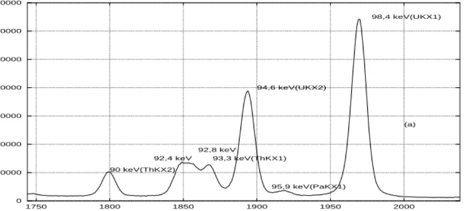
are superimposed (Fig. 1). 70 0 10000 20000 30000 40000 50000 60000 70000 1750 1800 1850 1900 1950 2000 90 keV(ThKX2) 94,6 keV(UKX2) 92,4 keV 92,8 keV 93,3 keV(ThKX1) 98,4 keV(UKX1) 95,9 keV(PaKX1) (a)
Figure 1: Principal useful X− and γ−rays in the spectral analysis of the KαX
region.
This region contains enough information to allow the determination of235U
71
and 238U and is sufficiently small for considering the efficiency as constant. It 72
is however very complex to analyze, due to several interfering X- and γ-rays. 73
These can be grouped as follows : 74
• 235U and daughters : 84.21 keV (γ231Th), 89.95 keV (γ231Th, T hK α2X), 75
92.28 keV (P aKα2X), 93.35 keV (T hKα1X), 95.86 keV (P aKα1X) 76
• 238U and daughters : 83.30 keV (γ234Th), 92.28 keV (P aK
α2X), 92.38 77
keV (γ234Th), 92.79 keV (γ234Th), 94.65 keV (U K
α2X), 95.86 keV (P aKα1X), 78
98.43 keV (U Kα1X), 99.85 keV (γ
234Pa)
79
• Uranium X-ray fluorescence : 94.65 keV (Kα2X), 98.43 keV(Kα1X). 80
In the standard approach, the processing of the considered region takes into 81
account the 3 elemental images, the first corresponding to235U and his
daugh-82
ters, the second to 238U and its daughters and the third to the uranium X-ray
83
fluoresence spectrum. These images are then represented by mathematical ex-84
pressions taking into account the shapes of the X-ray (Voigt profile) and γ-ray 85
(Gaussian) peaks, their energies, and intensities. The determination is then 86
carried out conventionally with a least squares method, like the MGA-U code
87
[1]. The final enrichment is obtained by correcting for the presence of 234U
88
with the 120.9 keV peak. 89
2.2
Experimental protocol
90
Six uranium oxide standards with different enrichments, from 0.7 to 9.6%, 91
and infinite thickness were counted several times by γ-ray spectrometry to 92
test the neural procedure. These were bare cylindrical pellets, with certified 93
enrichments and their main characteristics are presented in Table 1. 94
Table 1: Characteristics of U O2 standards
Diameter(cm)× Height(cm) U O ratio (g.g −1%) Stated enrich-ment (g.g−1%) 235U 235U +238U ratio (g.g−1%) 1,30× 2,00 88,00 0,7112 ±0,004 0,7112 1,30× 1,90 88,00 1,416 ±0,001 1,416 0,80× 1,10 88,00 2,785 ±0,004 2,786 0,80× 1,02 87,96 5,111 ±0,015 5,112 0,80× 1,00 87,98 6,222 ±0,018 6,225 0,92× 1,35 87,90 9,548 ±0,04 9,558
The Ge(HP) planar detector used in the measurement system had the 95
following specification : surface, 2.00 cm2 ; thickness, 1.00 cm ; FWHM, 190
96
eV at 6 keV and 480 eV at 122 keV. All the measurements were made under 97
the same conditions, i.e. with 0.05 keV per channel and a distance between 98
source and detector-window of 1.1 cm. Ten 20000-s. spectra for each standard 99
pellet were analysed by our procedure. The 234U concentration is relatively
100
low, although a 234235UU mass ratio varying from 0,5 to 1,1%, depending on the 101
pellet, was determined by γ-ray spectrometry by using both the 53.2 and the 102
120.9 keV peaks for 234U and the 185.7 keV peak for 235U . 103
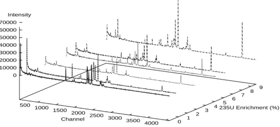
In short, 65 sets of experimental data from real-life experiments were pre-104
pared using the concentrations given in Table 1, and are illustrated in Fig. 105
2. 106
3
Layered Neural Network and Training method
107
3.1
Using Neural Networks
108
The purpose of this section, rather than the presentation of the neural network 109
theory, is to present the place of the connectionnist approach in γ-spectrometry 110
500 1000 1500 2000 2500 3000 3500 4000 0 1 2 3 4 5 6 7 8 9 0 10000 20000 30000 40000 50000 60000 70000 Channel 235U Enrichment (%) Intensity
Figure 2: 3D-Representation of the U O2 spectra set.
problems. Neural Networks are non-linear black-box model structures, to be 111
used with conventional parameter estimation methods. Most details and basic 112
concepts are clearly described in a paper to be published [12]. ANN consists 113
of a large number of neurons, i.e. simple linear or nonlinear computing el-114
ements, interconnected in complex ways and often organized into layers [6]. 115
The collective or parallel behaviour of the network is determined by the way 116
in which the nodes are connected and the relative type and strengh (excitory 117
or inhibitory) of the interactions among them [7]. 118
The objective of ANNs is to construct a suitable model which, when applied 119
to a 235U enrichment spectrum, produces an output, y, which approximates
120
the exact uranium enrichment ratio. The principal idea of the connectionist 121
approach is to substitute a neural model and the learning procedure of the net-122
work for classical fitting algorithms, which make use of complex mathematical 123
algorithms, generally based on the separation of a given curve, associated to 124
each individual peak, plus a background. 125
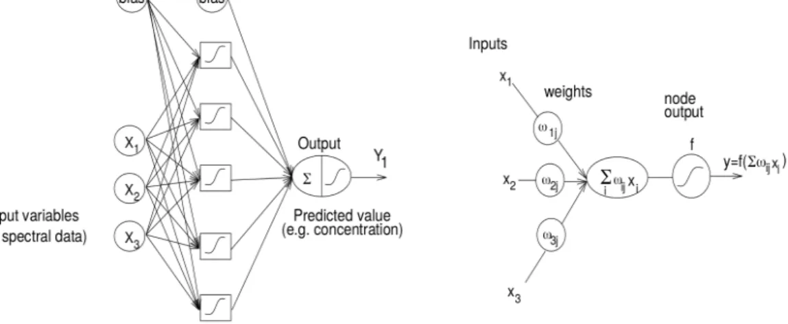
An exemple of multi-layer network is given in Fig. 3.a. The notation 126
convention is such that the square represents a computational unit into which 127
the input variables xj’s are fed and multiplied by the respective weights ωj’s.
128
The fundamental processing element of an ANN is a node (Fig. 3.b). Nodes are 129
analogous to neurons in biological systems. Each node has a series of weighted 130
inputs, ωi, which may be either an external signal or the output from other
131
nodes. The sum of the weighted inputs is transformed with a linear or a 132
non-linear transformation function (often the logistic function f (x) = 1+e1−x) . 133
In the statistical context, this standard Neural Network called Multi-Layered 134
Perceptron (MLP), is analogous to the Multivariate Nonlinear Regression. 135
Figure 3: (a) MLP 3-5-1 with nonlinear threshold and (b) schematic represen-tation of a node in an ANN.
Transmission of information between units of two neighboring layers is 136
performed through oriented links. These links are level-headed by connection 137
weights. The essential of the construction is as follows : 138
• input layer : this layer contains input units. Each unit receives input-139
variables, selected through a free parameters reduction procedure. 140
• hidden layer : this layer acts as an array of feature detectors picking 141
up features without regard to position. The information coming to the 142
input units is coded on the hidden layer into an internal representation 143
Thus, the input-layer units contribute to the input of each second-layer 144
unit. It is fully-connected to the output. 145
• output layer : it applies a sigmo¨ıd activation function to the weighted 146
sum of the hidden outputs. 147
The role of the hidden layer is fundamental. A network without hidden units 148
will be unable to perform the necessary multi-input multi-output mappings, 149
in particular with non-linear problems. Input pattern can always be encoded, 150
if there are enough hidden units, in a form so that the appropriate output 151
pattern can be generated from the corresponding input pattern. 152
The training data are denoted by χ = (x, yd)Nt=1 where N is the number 153
of observations and x is the feature vector corresponding to the tth obser-154
vation. The expected response yd = (y
1, y2, . . . yM) is related to the inputs
155
x = (x1, x2, . . . xN) according to
156
y = φ(x, ω), (1)
where ω are the connection weights. 157
The approximation results are non-constructive, and in practice the weights 158
have to be chosen to minimize some fitting criterion, e.g. least squares 159 J (ω) = 1 2 N X p (ypd− φ(xp, ω))2, (2)
with respect to all the parameters, where yd
p is the target for the pth example
160
pattern. The minimization has to be done by some numerical search procedure. 161
This is called nonlinear optimization. The parameter estimate is defined as 162
the minimizing argument : 163
ˆ
ω = argminωJ (ω) (3)
Most efficient search routines are based on local iteration along a ”downhill” 164
direction from the current point. We then have an iterative scheme of the 165 following kind : 166 ˆ ω(i+1) ← ˆω(i)− η × ∂J ∂ω(i) (4)
where ˆω(i) is the parameter estimate after iteration number i, η(> 0) is the
167
step size and ∂ω∂J(i) an estimate of the gradient of J (ω
i). The practical difference
168
between this device and the statistical version lies in the way the training data 169
are used to dictate the values for ω. It turns out that there are 2 main aspects 170
to the processing : (1) specifying the architecture of a suitable network, (2) 171
training the network to perform well with reference to a training set. 172
3.2
Application of the ANN
173
To check that this method was general and reliable, we have applied it to 65 174
sets of experimental data from real-life experiment : five 235U -pure idealized 175
spectra, and ten of each precited standard (see Table 1). Each spectrum 176
contains 4096 points. The computations of the spectra are compared on two 177
regression models: the MLP MODEL ( Fig. 3), where the inputs are spectral
178
data, and the MIXTURES OF EXPERTS MODEL(Fig. 4) [4] where the inputs are
179
the enrichment values. 180
The specifications for the networks created for the calibration of the sim-181
ulated data are listed in Table 2. They were found to be optimal according 182
to the rigourous methodology described in [12], for low prediction bias. The 183
choice of the right architecture is mainly intuitive and implies arbitrary deci-184
sions. But an attempt to apply ANN directly fails due to dimensionability. In 185
acccordance with this, the dimension of the input vector has been reduced dra-186
matically by Principle Components Analysis (PCA), leading to the adequate 187
Figure 4: Mixtures of Experts model.
reduction of weights emerging from the first layer of the ANN. 188
Table 2: ANNs specifications and parameters
parameter MLP 6-3-1 MLP 3-5-1 Mixtures of Experts Type of input spectral data spectral data enrichment value
input nodes 6 3 1
hidden node 3 5 1050
output node 1 1 210
learning rule BP BP Maximum Likelihood
input layer transfer function linear linear linear hidden layer transfer function sigmo¨ıdal sigmo¨ıdal sigmo¨ıdal output layer transfer function linear linear exponential
The MLP MODEL, depicted in Fig. 3, consists of an input layer of 6 or 3
189
units leading up through one layer of hidden units to an output layer of a single 190
unit that corresponds to the desired enrichment. This network represents a 191
poor parametrized model, but the training dataset (x; y(d))65
t=1 was small. The
192
network is initialized with random weights and trained. For each pattern, the 193
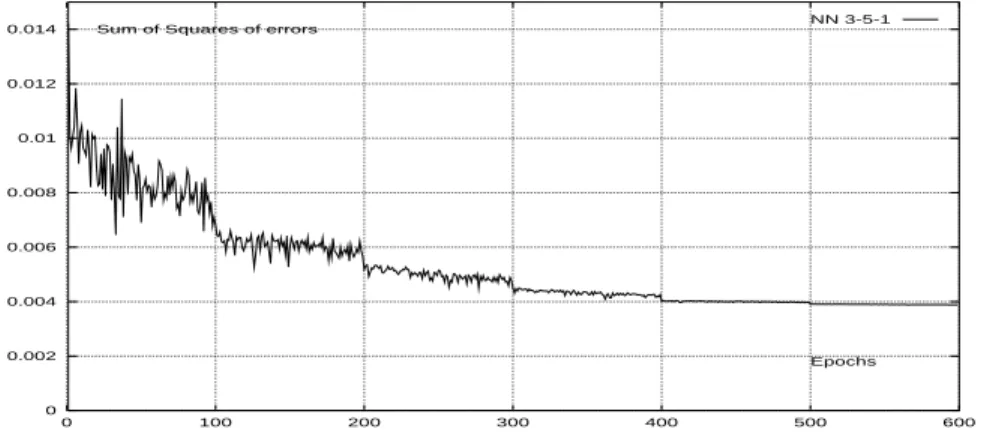
bias, Eq. 2, is evaluated. This quantity decreases rapidly (Fig. 5) in the 194
beginning, and the training is stopped when the network reaches a minimum 195
error on the training set, because this is an efficient way to avoid overfitting. 196
After 32 000 successful training passes, the bias rate range from -0.05 to 0.04% 197
for the 6-3-1 net (from -0.031 to 0.061% for the 3-5-1 net). 198
In the case of mixtures of experts (MEX), each item is associated with a 199
vector of measurable features, and a target yd which represents the enrich-200
ment. The network receives the input x and creates the output vector y as 201
0 0.002 0.004 0.006 0.008 0.01 0.012 0.014 0 100 200 300 400 500 600 Epochs Sum of Squares of errors NN 3-5-1
Figure 5: Sum of squares of bias on the training set for MLP architectures
a predicted value of the unknown yd. This model consists of 210
indepen-202
dant fully-connected networks (Fig. 4) : One expert is put for one channel of 203
the KαX region, each expert being an observer, trying to find a ”signal” due
204
to radioactive decay in a large amount of noise, the variance of each count 205
being proportional to the level and thus depending on the enrichment of a 206
particular sample and on the background level of the particular observation. 207
A cooperation-competition procedure driven by a supervisor between the ex-208
pert’s outputs leads to the choice of the most appropriate concentration. 209
Let y1, y2, . . . denote the output vectors of the experts, and g1, g2, . . .
210
the supervisor output units, then the output of the entire architecture, y, 211
is y = P210
i=1giyi. The supervisor decides whether expert i is currently
appli-212
cable or not. The winning expert is the network with the smallest bias (yd−y i).
213
214
4
Discussion of the Results using ANN
215
As the initial base included only 65 examples, we wanted to keep a maximum 216
of examples for the training base. Redundances in the data-set enrichments 217
present one main advantage : as we measure more than one response for each 218
case, information from all the measured responses can be combined to provide 219
more precise parameter estimation and to determine a more realistic model. 220
In all simulations, the measure of the system’s performance is the Mean 221
Square Error. The bias rates obtained by using MEX are benchmarked against 222
the results obtained by using MLPs in Table 3 and on Fig. 5 and Fig. 7. The 223
Fig. 5 shows the learning curves (i.e. the learning performances) for the two 224
MLP networks using a random training procedure. The horizontal axis gives 225
the number of epochs ; the vertical axis gives the Mean Square Errors value 226
(MSE). Clearly, the 6-3-1 network learned significantly faster than the 3-5-227
1. This difference can be explained by the information gain of the 6-inputs 228
network vs the 3-inputs network. 229
Table 3: Ranges of calculated Enrichments with MLP and MEX Declared enrich-ment MLP 3-5-1 MLP 6-3-1 MEXs 0.711% 0.691-0.723 0.700-0.720 0.702-0.710 1.416% 1.394-1.426 1.406-1.435 1.406-1.416 2.785% 2.732-2.822 2.762-2.799 2.784-2.790 5.111% 5.066-5.148 5.089-5.132 5.112-5.136 6.122% 6.105-6.162 6.117-6.133 6.088-6.112 9.548% 9.531-9.570 9.541-9.550 9.542-9.552
The Fig. 6 concerns the Multi-Expert model. The plotted points are pre-230
dicted enrichment value (one for each of the 210 experts) when a 5.111%−235U
231
spectrum is presented to the MEX model. The credit assignement procedure 232
on these 210 contributions is supervised to produce a final estimation. In the 233
right most column of Table 3, the final predicted values of the simulations with 234
MEX can be seen. Compared with the MLPs, this shows that MEX method is 235
really reliable ; for example, the bias between the predicted and the calculated 236
2.785% enrichments range from 2.784 to 2.790%. As noted above, after 32 237
000 successful training passes, the larger bias happens for 5.111 and 6.122% 238
enrichments. This relative lack of precision can be ascribed to the small size 239
of the training dataset. 240 4.6 4.8 5 5.2 5.4 5.6 5.8 6 6.2 6.4 50 100 150 200 Number of output-node Estimation of Uranium Enrichment
Figure 6: Example of enrichment value (at 5,785 %) predicted by the Mixtures of Experts
Fig. 7 compares the results of the three models. The bias between the 241
predicted and the desired enrichments is plotted for each of the 65 samples. 242
The darkest line is put for the MEX. The results suggest that the strong dis-243
persion of the bias with MLP is significantly attenuated when MEX is applied. 244
This judgement must be moderated for the 6.122-enrichment-ratio samples. A 245
comparison of the absolute bias curves suggest that, among of the three sys-246
tems studied, the Mixtures of Experts is capable of showing the most robust 247 performance. 248 -0.05 -0.04 -0.03 -0.02 -0.01 0 0.01 0.02 0.03 0.04 0.05 0.06 0 10 20 30 40 50 60 70 Number of spectrum Absolute error MLP 3-5-1 with normalized inputs
Figure 7: Absolute bias in the enrichment estimation
In fact, the modular approach presents three main advantages on the MLP 249
models: it is able to model behavior, it learns faster than a global model 250
and the representation is easier to interpret. The modular architecture takes 251
advantage of task decomposition, but the learner must decide which variables 252
to allocate to the networks. This method is, at the same time, very general 253
and very specific. It is very general in the sense that no hypothesis is made 254
on the aspect of the spectra : it does not depend on whether the spectra are 255
well resolved or not, whether they are very likely or not, whether you select 256
most significative areas of spectrum only (MLP models) or a global part of the 257
spectrum (MEX model). But, at the same time, the method is very specific 258
because the ANN must learn representative spectra of the family spectra to 259
identify. Furthermore, other tests proved to us that ANNs are resistant to 260
noise. Presently, we must put the blame on the excessively short size of the 261
training dataset. 262
5
Conclusion
263
The simulation studies on U O2 real spectra have shown that Neural Networks
264
can be very effective to predict 235U enrichment. They appear to be useful
265
when a fast response is needed with a reasonnable accuracy, when no hypoth-266
esis is made on the aspect of the spectra or when no definite mathematical 267
model can be assigned a priori. The resistance to noise is certainly one of the 268
most powerful characteristics of this method. Final network with connections 269
and weighting functions could be easily implemented using commercial digi-270
tal processing hardware. The good results obtained show that this method 271
can be considered at the state of art to produce quantitative estimates of 272
the concentrations of isotopic components in mixtures with fixed experimental 273
conditions : they may be better than those obtained with standard methods 274
in similar cases. This method has also been already successfully used in an 275
X-ray fluorescence application [11]. 276
There is no single learning procedure which is appropriate for all tasks. It is 277
of fundamental importance that special requirements of each task are analyzed 278
and that appropriate training algorithms are developed for families of tasks. 279
However, an efficient use of the networks requires as careful as possible analysis 280
of the problem, an analysis that is often ignored by impatient users. 281
Acknowlegments
282
The authors are extremely grateful to the staff of SAR and LPRI, and in 283
particular J.L. Boutaine, A.C. Simon and R. Junca for their support and 284
useful discussions during this work. V. Vigneron wishes to thank C. Fuche 285
from CREL for her support in this research. 286
References
287
[1] Gunning, R., Ruther, W. D., Miller, P., Goerten, J., Swinhoe, 288
M., Wagner, H., Verplancke, J., Bickel, M., and Abousahl, 289
S. MGAU: A new analysis code for measuring 235U enrichments in arbi-290
trary samples. Report UCRL-JC-114713, Lawrence Livermore National 291
Laboratory, (Livermore), 1994. 292
[2] Hagenauer, R. Non destructive uranium enrichment determination in 293
process holdup deposits. In Nucl. Mater. Manag. Proc (1991). 294
[3] Harry, R. J. S., Aaldijk, J. K., and Brook, J. P. Gamma spec-295
trometric determination of isotopic composition without use of standards. 296
In Report SM201/6 IAEA, Viena (1980). 297
[4] Jordan, M. I. Lectures on neural networks. Summer school, CEA-298
INRIA-EDF, MIT, 1994. Private Communication. 299
[5] Kull, L. A., Gonaven, R. O., and Glancy, G. E. A simple γ spec-300
trometric technique for measuring isotopic abundances in nuclear materi-301
als. Atomic Energy Review 144 (1976), 681–689. 302
[6] LeCun, Y. Efficient learning and second-order methods. Tech. rep., ATT 303
& Bell Laboratories, 1993. Private Communication. 304
[7] Martinez, J. M., Parey, C., and Houkari, M. Learning optimal 305
control using neural networks. In Proc. Fifth International Neuro-Nimes 306
(Paris, 1992), CEA (Saclay), EC2, pp. 431–442. 307
[8] Matussek, P. Accurate determination of the 235U isotope abundance 308
by γ spectrometry, a user’s manual for the certified reference material 309
EC-NMR-171/NBS-SRM-969. In Report KfK-3752 (Karlsruhe, 1985). 310
[9] Morel, J., Goenvec, H., Dalmazzone, J., and Malet, G. 311
R´ef´erences pour la d´etermination de l’uranium 235 dans les combustibles 312
nucl´eaires. IAEA Nuclear Safeguard Technology (1978). 313
[10] Reilly, T. D., Walton, R. B., and Parker, J. L. The enrichment 314
metter. In Report LA-4065-MS (Los Alamos, 1970). 315
[11] Simon, A. C., and Junca, R. Dosage de l’uranium et du pluto-316
nium par l’appareil de fluorescence X SAPRA γX/Ir: simplification 317
des codes de calcul dans le cas de solutions pures. In Note technique 318
DTA/DAMRI/SAR/S/94-433 (Saclay, 1994). 319
[12] Vigneron, V., and Martinez, J. M. A looking at Neural Network 320
methodology. Submitted to Nuclear Instruments and Methods in Physics 321
Research (1995). 322
List of Figures
323
1 Principal useful X− and γ−rays in the spectral analysis of the 324
KαX region. . . 3
325
2 3D-Representation of the U O2 spectra set. . . 5
326
3 (a) MLP 3-5-1 with nonlinear threshold and (b) schematic rep-327
resentation of a node in an ANN. . . 6 328
4 Mixtures of Experts model. . . 8 329
5 Sum of squares of bias on the training set for MLP architectures 9 330
6 Example of enrichment value (at 5,785 %) predicted by the Mix-331
tures of Experts . . . 10 332
7 Absolute bias in the enrichment estimation . . . 11 333


![Synthèse énantiosélective du [7]hélicène à l’aide de la réaction de fermeture de cycle par métathèse d’oléfine asymétrique et synthèse de binaphtols via une réaction de couplage oxydatif](data:image/gif;base64,R0lGODlhAQABAIAAAP///wAAACH5BAEAAAAALAAAAAABAAEAAAICRAEAOw==)