HAL Id: hal-00295825
https://hal.archives-ouvertes.fr/hal-00295825
Submitted on 25 Jan 2006
HAL is a multi-disciplinary open access
archive for the deposit and dissemination of
sci-entific research documents, whether they are
pub-lished or not. The documents may come from
teaching and research institutions in France or
abroad, or from public or private research centers.
L’archive ouverte pluridisciplinaire HAL, est
destinée au dépôt et à la diffusion de documents
scientifiques de niveau recherche, publiés ou non,
émanant des établissements d’enseignement et de
recherche français ou étrangers, des laboratoires
publics ou privés.
atmospheric CO2 inversions: a quantitative assessment
C. Rödenbeck, T. J. Conway, R. L. Langenfelds
To cite this version:
C. Rödenbeck, T. J. Conway, R. L. Langenfelds. The effect of systematic measurement errors on
at-mospheric CO2 inversions: a quantitative assessment. Atat-mospheric Chemistry and Physics, European
Geosciences Union, 2006, 6 (1), pp.149-161. �hal-00295825�
www.atmos-chem-phys.org/acp/6/149/ SRef-ID: 1680-7324/acp/2006-6-149 European Geosciences Union
Chemistry
and Physics
The effect of systematic measurement errors on atmospheric CO
2
inversions: a quantitative assessment
C. R¨odenbeck1, T. J. Conway2, and R. L. Langenfelds3
1Max Planck Institute for Biogeochemistry, Jena, Germany
2NOAA Climate Monitoring and Diagnostics Laboratory, Boulder CO, USA
3CSIRO Marine and Atmospheric Research, Australia
Received: 25 July 2005 – Published in Atmos. Chem. Phys. Discuss.: 20 September 2005 Revised: 12 December 2005 – Accepted: 12 December 2005 – Published: 25 January 2006
Abstract. Surface-atmosphere exchange fluxes of CO2,
es-timated by an interannual atmospheric transport inversion from atmospheric mixing ratio measurements, are affected by several sources of errors, one of which is experimental errors. Quantitative information about such measurement er-rors can be obtained from regular co-located measurements done by different laboratories or using different experimen-tal techniques. The present quantitative assessment is based on intercomparison information from the CMDL and CSIRO atmospheric measurement programs. We show that the ef-fects of systematic measurement errors on inversion results are very small compared to other errors in the flux estima-tion (as well as compared to signal variability). As a prac-tical consequence, this assessment justifies the merging of data sets from different laboratories or different experimental techniques (flask and in-situ), if systematic differences (and their changes) are comparable to those considered here. This work also highlights the importance of regular intercompari-son programs.
1 Introduction
Regular mixing ratio measurements of an atmospheric trace gas contain information about spatial and temporal variations in its sources and sinks. A way to infer these flux variations is the atmospheric transport inversion technique. This assess-ment focuses on CO2, which has been measured by several institutions at over 100 sites worldwide (e.g., Conway et al., 1994; Francey et al., 2003; see also GLOBALVIEW-CO2, 2004). Based on these data, several global interannual inver-sion studies have been conducted (e.g., Rayner et al., 1999; Bousquet et al., 2000; R¨odenbeck et al., 2003; Peylin et al., 2005; Baker et al., 2006). Flux estimates obtained by the Correspondence to: C. R¨odenbeck
(christian.roedenbeck@bgc-jena.mpg.de)
inversion technique, however, are affected by errors of three types:
1. Transport model errors. The transport model – one of the most important elements of the calculation – does not simulate the correct atmospheric tracer concentra-tion fields, even if the correct flux fields would be sup-plied. This is due to errors in the parameterizations (especially vertical mixing) and meteorological input data, but also due to the relatively coarse model grids (coarse compared to the spatial structures in circulation and source processes, and especially coarse compared to the point measurements of mixing ratios).
2. Methodology and assumptions. Due to the current spa-tial density of observation sites, fluxes in several parts of the world cannot be well constrained by the avail-able atmospheric information alone. In order to make the inverse problem mathematically well-posed, a-priori information about the fluxes is supplied, either in the form of a-priori estimates or of assumed uncertainty pat-terns and correlation structure (“flux model”), or both. Present understanding of surface processes is compat-ible with a large range of such choices, which results in a large range of flux estimates. Also, any choice of (further) mathematical regularization methods can lead to different results.
3. Experimental errors. Even with present-day
high-precision methodology and equipment, the mixing ratio data themselves are subject to experimental errors dur-ing sampldur-ing, storage, extraction, and analysis (Masarie et al., 2001b). While random errors tend to average out when looking at longer time scales (such as interannual variability), systematic errors will not. Offsets could also occur between measurements by different labora-tories (Masarie et al., 2001a).
In addition to the flux estimates, the Bayesian inversion framework yields uncertainty intervals. They are calculated by error propagation from the assumed magnitudes of the above-mentioned errors. However, many of these uncertain-ties are very poorly known. Moreover, error propagation as-sumes random errors, while systematic errors are potentially even more important. A more complete picture of the errors can be obtained from “sensitivity testing”: Transport model errors (“type 1”) are (partially) assessed by comparison of re-sults obtained with different transport models (e.g., Gurney
et al., 2002; Baker et al., 2006; Rivier et al., 20061), while
errors related to methodology and assumptions (“type 2”) are (again partially) revealed by the differences between differ-ent inversion setups or differdiffer-ent studies (e.g., Bousquet et al., 2000; R¨odenbeck et al., 2003). Even though sensitivity test-ing can only yield a lower limit to all the potential errors, it turns out that these errors can be large, at least with respect to certain modes of variability (e.g., long-term spatial flux patterns, compare Bousquet et al., 2000; R¨odenbeck et al., 2003). So far, measurement errors have generally only been treated as random and uncorrelated.
This study attempts a quantitative assessment of system-atic errors of “type 3”: What is the effect of systemsystem-atic ex-perimental errors, compared to the other errors, on a global
interannual CO2 inversion? In particular, what flux errors
arise from systematic differences between measurements by different experimental methods or different laboratories?
2 Method
The present assessment of errors of “type 3” is done, as in the case of the other errors, in the form of a sensitivity com-parison. The inversion methodology, including the particu-lar set-up used here, is described in R¨odenbeck (2005). It is similar to the one used in R¨odenbeck et al. (2003). An important difference is the use of data with higher time res-olution. Rather than monthly mean data and fluxes, data are used as individual values (flask pair mean, or hourly mean, respectively, for flask and in-situ measurements), and fluxes are estimated nominally on a daily time step. More informa-tion on the inversion set-up is found in the Appendix.
The sensitivity comparison uses different records of
atmo-spheric CO2 mixing ratios observed at the same site. The
differences between such records are taken as representative of the experimental errors. Two alternatives are considered:
– At some observation sites, CO2mixing ratios are
mea-sured by different techniques, such as by air sampling in 1Rivier, L., Bousquet, P., Brandt, J., Ciais, P., Geels, C., Gloor, M., Heimann, M., Karstens, U., Peylin, P., and R¨odenbeck, C.: Comparing Atmospheric Transport Models for Regional Inversions over Europe. Part 2: Estimation of the regional sources and sinks of CO2using both regional and global atmospheric models, in prepa-ration, 2006.
glass flasks analyzed in a central laboratory, and by con-tinuous in-situ measurements (Tans et al., 1990; Steele et al., 2004). These co-located records represent essen-tially independent measurements, except that both use reference gases that are traceable to the same primary standards. Therefore, any difference between a flask pair mean and the coincidental hourly mean from the continuous analyzer may be considered as representing all experimental errors relevant for the inversion calcu-lation.
– There are also sites where CO2 mixing ratios are
ob-served by different institutions. At some of these sites, air samples are intentionally collected by two institu-tions close to simultaneously, independently from each other using their respective sampling procedures, and analyzed by their respective laboratories (Masarie et al., 2001a). As before, differences between such simultane-ous values can be expected to give an indication of the full range of potential experimental errors. In addition, they may specifically quantify potential offsets between the measurement networks of different institutions as a whole.
From these measured differences, several scenarios of con-centration differences at all sites used in the flux estimation are derived, as detailed below. The inversion algorithm is then used to calculate the flux differences that result in re-sponse to these measurement differences. Exploiting the fact that the flux estimates depend linearly on the data, the ampli-tude of the flux differences quantifies the implied flux error. These errors are then set into perspective by comparison with the other types of error of the inversion method.
2.1 Assessment A: flask/in-situ differences
Differences between flask and continuous in-situ measure-ments are considered at Point Barrow [BRW], Mauna Loa [MLO], Samoa [SMO], and South Pole [SPO] (NOAA/CMDL Baseline Observatories) and at the Cape
Grim Baseline Air Pollution Station [CGA] (CSIRO data2).
At Cape Grim, a further comparison is possible involving parallel measurements obtained by CSIRO using two inde-pendent in-situ analyzers (the conventional system based on a Siemens Ultramat 5E used here, and a new LoFlo system;
Steele et al., 2004); however, as CO2differences are slightly
smaller than observed between flask and continuous mea-surements, it is not considered any further here.
In assessment A1, a record of mixing ratio differences (co-incidental hourly mean minus flask pair mean) is formed for each of the 5 sites. These records are then low-pass filtered 2The Cape Grim Baseline Air Pollution Station is funded and managed by the Australian Bureau of Meteorology, and the scien-tific program is jointly supervised with CSIRO Marine and Atmo-spheric Research.
-2.5 -2 -1.5 -1 -0.5 0 0.5 1 1.5 1995 1996 1997 1998 1999 2000 2001 2002
CO2 conc. diff. (ppm)
year (A.D.) -0.3 -0.2 -0.1 0 0.1 0.2 0.3 1995 1996 1997 1998 1999 2000 2001 2002
CO2 conc. diff. (ppm)
year (A.D.) BRW CGA MLO SMO SPO
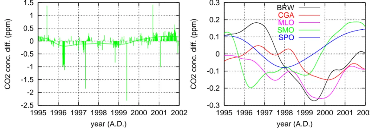
Fig. 1. Left: Concentration differences between flask pair averages and coincident hourly mean values from the continuous analyzer at Samoa (SMO), measured by NOAA/CMDL. The impulses give the individual values, while the curve gives differences smoothed on a one year time scale. Right: Smoothed concentration differences between flask pair averages and coincident hourly mean values at the sites contributing to assessment A.
on a time scale of one year. The resulting smooth curves are considered as a representation of the systematic part of ex-perimental errors (Tans et al., 1990). The left panel of Fig. 1 shows, as an example, the differences for SMO, both as in-dividual values and filtered, while the right panel gives the systematic parts at all observatories. These smooth curves are now sub-sampled at the times of the original flask mea-surements. An inversion is conducted that uses these differ-ence records at BRW, CGA, MLO, SMO, and SPO, and zero difference (i.e., a zero value at each respective original sam-pling time) for all other sites. Clearly, this test will only give meaningful flux differences within the regions of influence of BRW, CGA, MLO, SMO, and SPO.
The chosen way to filter out the systematic error is clearly not unique. Therefore, in a variant of this assessment (A2), two full inversion calculations are done, one based on flask data exclusively, and one with the continuous records sub-stituting for the flask records at BRW, CGA, MLO, SMO, and SPO. Then the resulting flux estimates are subtracted from each other. These flux differences not only reflect any systematic differences between the measurements, but also the different sampling times: the sampled air parcels and their origins are not identical. (Note that the trivial influ-ence of different sampling densities in time is intentionally minimized by the applied data density weighting explained in the Appendix.)
2.2 Assessment B: inter-laboratory differences
Coincidental air sampling as mentioned above is done regu-larly by NOAA/CMDL and CSIRO at several sites (Masarie et al., 2001a). Here, measured differences at Cape Grim (CGA-CGO) are used. Similar to assessment A, a record of differences is formed (CSIRO flask pair mean minus NOAA/CMDL flask pair mean, for those occasions where
both of them exist, are used in the standard inversion, and are taken within maximally 1 h from each other). This dif-ference record is then filtered (again one year time scale) to get the “systematic part”, shown in the left panel of Fig. 2. (In the framework of the intercomparison program, one flask of each pair sampled by NOAA/CMDL is also first analyzed in the CSIRO laboratory, to obtain additional information on the respective role of sampling and analysis in the origin of differences (Masarie et al., 2001a). Here, the difference be-tween both flask pair means is taken, because this seems to comprise the relevant difference as seen by the inversion
cal-culation)3.
The aim of assessment B is to obtain quantitatively the flux differences in response to potential systematic offsets be-tween the two networks, in an inversion calculation using the combined CMDL and CSIRO data sets. This requires con-centration differences to be supplied at all these sites. There-fore, the “systematic part” of the CGA-CGO differences is taken as a proxy for the systematic differences between the CMDL and CSIRO sampling networks as a whole. The de-gree to which this is justified can be checked by the right panel of Fig. 2 which compares the systematic parts at Alert (ALC-ALT), Cape Grim (CGA-CGO), Mauna Loa (MLU-MLO), and South Pole (SPU-SPO): All four curves exhibit a general downward trend (especially during 1995 and 1997), but also several site-specific features.
3At some sites, there may be sources of experimental error that are common to both labs and do not appear in the difference (e.g., due to artefacts involving common air intakes, or due to un-usual flask storage conditions such as low ambient pressure and long storage times at South Pole). However, based on other in-formation about consistency among sites within the same network and through the intercomparisons, such errors over and above the CSIRO-CMDL differences are expected to be very small by com-parison.
-1 -0.8 -0.6 -0.4 -0.2 0 0.2 0.4 0.6 0.8 1 1995 1996 1997 1998 1999 2000 2001 2002
CO2 conc. diff. (ppm)
year (A.D.) -0.3 -0.2 -0.1 0 0.1 0.2 0.3 1995 1996 1997 1998 1999 2000 2001 2002
CO2 conc. diff. (ppm)
year (A.D.)
ALC-ALT
CGA-CGO
MLU-MLO SPU-SPO
Fig. 2. Left: Concentration differences between flask pair values measured by CMDL and CSIRO at Cape Grim (CGA-CGO). The impulses
give the individual values, while the curve gives differences smoothed on a one year time scale. Right: Smoothed concentration differences between CMDL and CSIRO measurements at four intercomparison sites.
It should be noted that part of the systematic difference is understood. Both laboratories’ data are referenced against a common scale maintained by CMDL in its role as the
WMO Central CO2Calibration Laboratory (CCL)4. Recent
re-evaluation of past calibration assignments by the CCL in-dicates that part (≈0.1 ppm) of the change in the CSIRO-CMDL difference observed in Fig. 2 is due to a combination of a small drift towards higher concentrations in CSIRO’s primary standards and the need for adjustment of CCL as-signments made during the early part of the measurement period considered here.
In the test inversion, records for all CMDL and CSIRO sites are created by sub-sampling the smooth CGA-CGO dif-ferences curve at the respective site’s sampling instants. Two cases are then considered: In assessment B1a, the smooth CGA-CGO concentration difference is applied to all CSIRO sites, while at CMDL sites zero values are used. Conversely, in B1c the difference is put to all CMDL sites, and zero to CSIRO sites. In both cases, at the sites Alert (ALT), Cape Grim (CGA), Mauna Loa (MLO), and South Pole (SPO) (where records from both laboratories exist) half the smooth CGA-CGO difference is used, envisaging that the offset could be reduced by averaging there. It should be noted that this usage of the intercomparison difference is not meant to refer to any “data correction”. Rather, assessments B1a/c just quantify the magnitude and structure of the effect on es-timated fluxes. This aim is also reflected in the choice of a twin assessment which is symmetric with respect to the two laboratories (including using the difference with equal sign in both cases).
4The CCL maintains the WMO scale using a manometric tech-nique that should be accurate in absolute terms to better than ±0.1 ppm, and propagates the scale to other WMO laboratories by providing them with CO2assignments to their primary air standards (Zhao et al., 1997).
However, spurious flux differences not only arise from systematic offsets between groups of sites (i.e., implied sys-tematic concentration differences in space). As soon as such a (time-varying) offset exists, it has an effect even if only one network is used (i.e., also without any spatial gradients), be-cause any coherent time variations at all sites falsely imply changes in total atmospheric carbon content and thus lead to spurious fluxes. In order to separate the temporal and the spa-tial effect of the offset, assessment B2 is performed. There, the smooth CGA-CGO concentration difference is applied to all sites of both laboratories. The results of this assess-ment will also reflect regional flux differences due to the fact that concentrations at different sites are sampled at different times.
2.3 Comparison assessment C: model errors
To put the results of the previous assessments into perspec-tive, assessment C indicates the order of magnitude (lower limit) of model errors. Flux differences are calculated for two spatial resolutions of the transport model: Standard
reso-lution (≈4◦latitude×5◦longitude×19 vertical levels) or
en-hanced resolution (≈1.8◦ latitude×1.8◦ longitude×28
ver-tical levels). Specifically, a flux field comprising all
ma-jor CO2components is supplied (fossil fuel emissions from
Olivier et al., 2001, terrestrial NEE from a Biome-BGC model simulation – Churkina and Trusilova, 2002, daily val-ues – and ocean-atmosphere exchange from Takahashi et al., 2002 and Gloor et al., 2003); the exact choice is not crucial here. These fluxes are transported by the tracer model on the two resolutions, and the simulated concentrations are sam-pled at the same locations and times as in assessments A and B (flask sites). The concentration differences between both simulations (standard minus enhanced resolution) are then directly fed into the inversion calculation.
-0.5 -0.4 -0.3 -0.2 -0.1 0 0.1 0.2 0.3 0.4 0.5 0.6 1995 1996 1997 1998 1999 2000 2001 2002
CO2 conc. diff. (ppm)
year (A.D.) -35 -30 -25 -20 -15 -10 -5 0 5 10 1995 1996 1997 1998 1999 2000 2001 2002
CO2 conc. diff. (ppm)
year (A.D.)
Fig. 3. Concentration differences between transport model simulations using standard resolution (≈4◦latitude×5◦longitude×19 vertical levels) and enhanced resolution (≈1.8◦latitude×1.8◦longitude×28 vertical levels). Left: Cape Grim (CGA); Right: Hegyhatsal (HUN).
Figure 3 gives two examples of these concentration differ-ences, where Cape Grim (CGA) represents a typical order of magnitude, while Hegyhatsal (HUN) exhibits the largest differences of all considered sites. Clearly, these differences can only yield a lower limit to model errors, as the numer-ical parameterizations and meteorolognumer-ical data are identnumer-ical between the two model runs. The total model error, due to all the reasons mentioned in the Introduction, is expected to be much larger (see, e.g., systematic differences up to several ppm between model simulations by different transport mod-els at continental sites in Europe presented in Gemod-els et al.,
20065).
3 Results and discussion
The flux differences that arise from the concentration dif-ferences defined in the described assessments A and B, are
shown in Fig. 4. They are integrated over different
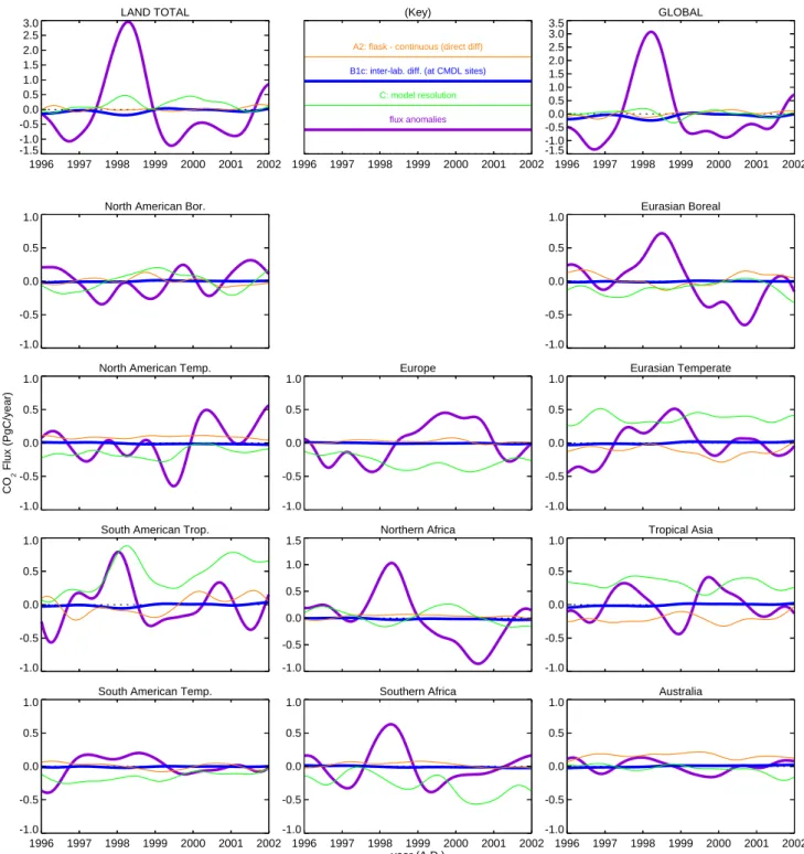
re-gions, deseasonalized, and filtered for interannual variations. The absolute difference in the global flux does not exceed 0.3 PgC/yr for any of these cases related to measurement er-rors. Maximum absolute differences at the spatial scale of the TransCom-3 regions are mostly about 0.1 PgC/yr. In all regions, these flux differences are very small compared to the systematic errors of “type 2” found by sensitivity testing (e.g. R¨odenbeck, 2005, for the set-up used here) or by comparison with other inversion studies. As shown in Fig. 5, in most re-gions the differences are smaller or much smaller than the considered resolution part of the model error (assessment C as lower limit to errors of “type 1”). They are also very small 5Geels, C., Bousquet, P., Ciais, P., Gloor, M., Peylin, P., Ver-meulen, A. T., Dargaville, R., Brandt, J., Christensen, J. H., Frohn, L. M., Heimann, M., Karstens, U., R¨odenbeck, C., and Rivier, L.: Comparing Atmospheric Transport models for regional inversions
over Europe. Part 1: Mapping the CO2 atmospheric signals, in
preparation, 2006.
compared to the inferred magnitude of interannual variabil-ity, i.e., the signal itself. Taking the temporal standard devia-tion of the individual time series in Fig. 5 as a rough measure of the amplitude of their interannual variations, Fig. 6 (solid bars) summarizes this ranking.
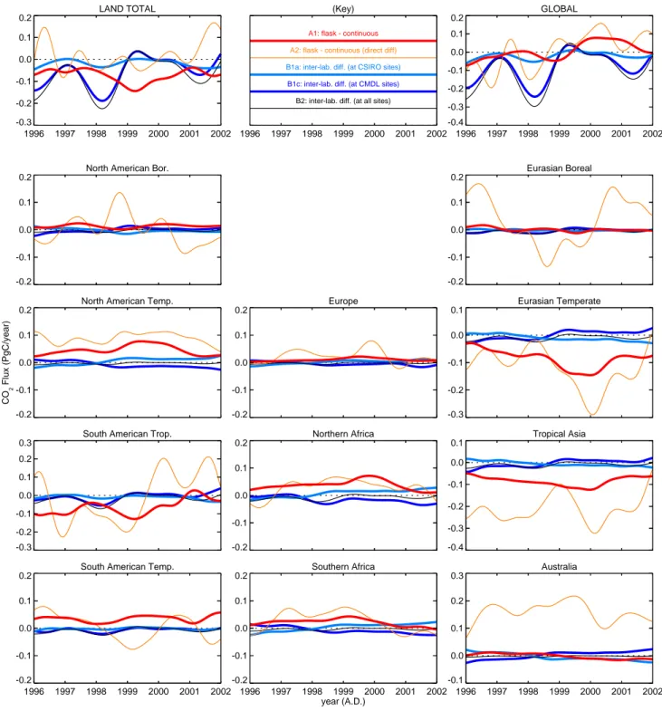
Looking into the individual assessments shown in Fig. 4, measurement differences between experimental methods (Fig. 1, assessment A) and between institutions (Fig. 2, as-sessment B) are similar, and lead to flux differences of the same order of magnitude in most regions. This suggests that all these data records are qualitatively equivalent with respect to their use in inversion calculations. Globally averaged flux differences in Fig. 4 are smaller for assessment A than B be-cause for A errors are applied only to the 5 sites with ob-served continuous-flask differences.
Further, flux differences under assessments B1a/c (con-centration offset applied to either the CMDL or the CSIRO network) are not dramatically larger than those under B2 (same offset applied everywhere). To the extent that offsets between measurement networks are on the same order as sys-tematic measurement errors, this means that errors from the merging of data from different sources do not significantly exceed errors present anyway as soon as systematic concen-tration differences exist, even within the same network. The larger differences for assessment B1c compared to B1a only reflect the larger number of sites in the NOAA/CMDL net-work.
Finally, assessment A2 (direct flux difference which also reflects the different measurement schedules) leads to larger and more variable differences than A1 (inverting smoothed concentration differences only). This reveals that, even for the interannual variations in coarse regions considered here, the flux differences caused by experimental errors are ex-ceeded by the influence of the measurement schedule (i.e., by differences in which particular air parcels have been sam-pled). If fluxes are considered at finer temporal and spatial
LAND TOTAL 1996 1997 1998 1999 2000 2001 2002 -0.3 -0.2 -0.1 0.0 0.1 0.2
North American Bor.
-0.2 -0.1 0.0 0.1 0.2
North American Temp.
-0.2 -0.1 0.0 0.1 0.2 CO 2 Flux (PgC/year)
South American Trop.
-0.3 -0.2 -0.1 0.0 0.1 0.2 0.3
South American Temp.
1996 1997 1998 1999 2000 2001 2002 -0.2 -0.1 0.0 0.1 0.2 (Key) 1996 1997 1998 1999 2000 2001 2002
B2: inter-lab. diff. (at all sites) B1c: inter-lab. diff. (at CMDL sites)
B1a: inter-lab. diff. (at CSIRO sites)
A2: flask - continuous (direct diff) A1: flask - continuous
Europe -0.2 -0.1 0.0 0.1 0.2 Northern Africa -0.2 -0.1 0.0 0.1 0.2 Southern Africa 1996 1997 1998 1999 2000 2001 2002 year (A.D.) -0.2 -0.1 0.0 0.1 0.2 GLOBAL 1996 1997 1998 1999 2000 2001 2002 -0.4 -0.3 -0.2 -0.1 0.0 0.1 0.2 Eurasian Boreal -0.2 -0.1 0.0 0.1 0.2 Eurasian Temperate -0.3 -0.2 -0.1 0.0 0.1 Tropical Asia -0.4 -0.3 -0.2 -0.1 0.0 0.1 Australia 1996 1997 1998 1999 2000 2001 2002 -0.1 0.0 0.1 0.2 0.3
Fig. 4. Flux differences estimated in response to the considered scenarios A and B of concentration differences. Fluxes are deseasonalized
and filtered for interannual frequencies. The panels refer to different regions: Part I. Fluxes integrated over the TransCom 3 land regions, plus land and global totals. (The vertical scale can change between panels, but the tic interval is always the same.)
resolution, the effect of higher sampling density is expected to become larger.
It must be noted that these results are specific in a num-ber of ways. First, they are specific to the inversion set-up chosen here. Depending especially on the particular choices
of uncertainties and uncertainty patterns (which imply dif-ferent susceptibilities of regional fluxes with respect to the concentration signals at the individual sites), the same con-centration differences might lead to other flux differences in other inversion configurations. However, changes in these
OCEAN TOTAL 1996 1997 1998 1999 2000 2001 2002 -0.3 -0.2 -0.1 0.0 0.1 0.2
North Pacific Temp.
-0.1 0.0 0.1 0.2
West Pacific Tropics
-0.1 0.0 0.1 0.2 CO 2 Flux (PgC/year)
East Pacific Tropics
-0.2 -0.1 0.0 0.1
South Pacific Temp.
1996 1997 1998 1999 2000 2001 2002 -0.1 0.0 0.1 0.2 (Key) 1996 1997 1998 1999 2000 2001 2002
B2: inter-lab. diff. (at all sites) B1c: inter-lab. diff. (at CMDL sites)
B1a: inter-lab. diff. (at CSIRO sites)
A2: flask - continuous (direct diff) A1: flask - continuous
Northern Ocean
-0.1 0.0 0.1 0.2
North Atlantic Temp.
-0.1 0.0 0.1 0.2 Atlantic Tropics -0.1 0.0 0.1 0.2
South Atlantic Temp.
1996 1997 1998 1999 2000 2001 2002 year (A.D.) -0.1 0.0 0.1 0.2 GLOBAL 1996 1997 1998 1999 2000 2001 2002 -0.4 -0.3 -0.2 -0.1 0.0 0.1 0.2
Indian Trop. Ocean
-0.2 -0.1 0.0 0.1
S.Indian Temp. Ocean
-0.2 -0.1 0.0 0.1 Southern Ocean 1996 1997 1998 1999 2000 2001 2002 -0.1 0.0 0.1 0.2
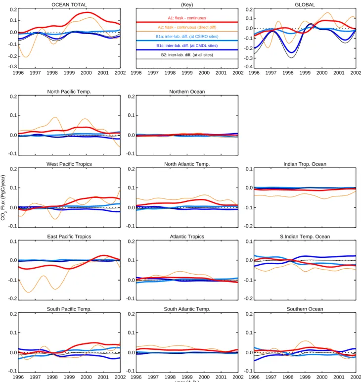
Fig. 4. Part II. Fluxes integrated over the TransCom 3 ocean regions, plus ocean and global totals.
susceptibilities affect concentration signals and errors in sim-ilar ways. Therefore, the finding that the calculated flux dif-ferences are small compared to other errors, as well as to the signals of interest, is expected to also be true in other inversions. To illustrated this, Fig. 6 compares the standard results with those from an inversion set-up where all a-priori
σ-intervals of the fluxes have been decreased by a factor of
√
8 (i.e., µ=8 in the notation of R¨odenbeck, 2005). This exemplary set-up change represents a relatively large manip-ulation. The resulting stronger damping is seen to reduce the interannual variability in both the flux signal and the var-ious error components, while indeed essentially preserving their mutual ranking. In fact, the relative decrease in ampli-tude is mostly even stronger for the errors than for the signal,
LAND TOTAL 1996 1997 1998 1999 2000 2001 2002 -1.5 -1.0 -0.5 0.0 0.5 1.0 1.5 2.0 2.5 3.0
North American Bor.
-1.0 -0.5 0.0 0.5 1.0
North American Temp.
-1.0 -0.5 0.0 0.5 1.0 CO 2 Flux (PgC/year)
South American Trop.
-1.0 -0.5 0.0 0.5 1.0
South American Temp.
1996 1997 1998 1999 2000 2001 2002 -1.0 -0.5 0.0 0.5 1.0 (Key) 1996 1997 1998 1999 2000 2001 2002 flux anomalies C: model resolution
B1c: inter-lab. diff. (at CMDL sites)
A2: flask - continuous (direct diff)
Europe -1.0 -0.5 0.0 0.5 1.0 Northern Africa -1.0 -0.5 0.0 0.5 1.0 1.5 Southern Africa 1996 1997 1998 1999 2000 2001 2002 year (A.D.) -1.0 -0.5 0.0 0.5 1.0 GLOBAL 1996 1997 1998 1999 2000 2001 2002 -1.5 -1.0 -0.5 0.0 0.5 1.0 1.5 2.0 2.5 3.0 3.5 Eurasian Boreal -1.0 -0.5 0.0 0.5 1.0 Eurasian Temperate -1.0 -0.5 0.0 0.5 1.0 Tropical Asia -1.0 -0.5 0.0 0.5 1.0 Australia 1996 1997 1998 1999 2000 2001 2002 -1.0 -0.5 0.0 0.5 1.0
Fig. 5. As Fig. 4, but comparison of the largest flux differences from scenarios A and B with the flux differences from scenario C, as well
as with the flux anomalies themselves. Part I. Land regions.
probably because the specified a-priori time correlations be-come more efficient in damping high-frequency error com-ponents (cases A2 and C). This can be taken as a hint that the more rigid set-up, even though its ability to fit the data deteriorates, may have a better balance between information
loss and error damping than the standard set-up6.
6We note in passing that in some regions the model errors are almost of comparable order than the flux signal (Figs. 5 and 6), in broad agreement with the significance tests by Baker et al. (2006). In the more strongly damped set-up, the situation is improved.
OCEAN TOTAL 1996 1997 1998 1999 2000 2001 2002 -0.5 0.0 0.5 1.0
North Pacific Temp.
-0.5 0.0 0.5 1.0
West Pacific Tropics
-0.5 0.0 0.5 1.0 CO 2 Flux (PgC/year)
East Pacific Tropics
-1.0 -0.5 0.0 0.5
South Pacific Temp.
1996 1997 1998 1999 2000 2001 2002 -1.0 -0.5 0.0 0.5 (Key) 1996 1997 1998 1999 2000 2001 2002 flux anomalies C: model resolution
B1c: inter-lab. diff. (at CMDL sites)
A2: flask - continuous (direct diff)
Northern Ocean
-0.5 0.0 0.5 1.0
North Atlantic Temp.
-0.5 0.0 0.5 1.0 Atlantic Tropics -1.0 -0.5 0.0 0.5
South Atlantic Temp.
1996 1997 1998 1999 2000 2001 2002 year (A.D.) -1.0 -0.5 0.0 0.5 GLOBAL 1996 1997 1998 1999 2000 2001 2002 -1.5 -1.0 -0.5 0.0 0.5 1.0 1.5 2.0 2.5 3.0 3.5
Indian Trop. Ocean
-0.5 0.0 0.5 1.0
S.Indian Temp. Ocean
-0.5 0.0 0.5 1.0 Southern Ocean 1996 1997 1998 1999 2000 2001 2002 -0.5 0.0 0.5 1.0
Fig. 5. Part II. Ocean regions.
Second, the flux differences depend on the time and space scales chosen for investigation. Here we selected those scales that were used for interpretation e.g. in R¨odenbeck et al. (2003). The impact increases for smaller scales, but, again, the other types of errors behave in a similar way. However, if very different aspects (e.g., seasonal cycle amplitudes) are considered, a specific assessment might be necessary.
Finally, the presented results refer to the specific data sets and measurement networks used here. However, other inter-comparisons of measurements by independent institutions have revealed differences of the same order as those used here (e.g., comparison at Alert (ALT) between MSC (Mete-orological Service of Canada) and CMDL, Fig. 4 of Masarie et al., 2001b), which would therefore correspond to similar
Ocean
0.0 0.1 0.2
Southern Ocean
South Pacific Temp. South Atlantic Temp.
S.Indian Temp. Ocean
West Pacific Tropics East Pacific Tropics
Atlantic Tropics
Indian Trop. Ocean North Pacific Temp. North Atlantic Temp.
Northern Ocean Land 0.0 0.1 0.2 0.3 0.4 0.5 SD of CO 2 Flux (PgC/year)
South American Temp.
Australia
South American Trop.
Southern Africa Northern Africa Tropical Asia
North American Temp.
Eurasian Temperate North American Bor.
Europe Eurasian Boreal Totals 0.0 0.5 1.0 1.5 GLOBAL LAND TOTAL OCEAN TOTAL flux anomalies C: model resolution
B1c: inter-lab. diff. (at CMDL sites) A2: flask - continuous (direct diff)
Fig. 6. Solid bars: Temporal standard deviations of the interannually filtered time series shown in Fig. 5. Hollow bars: Same as solid bars,
but using an inversion set-up with increased damping of the flux signals (all a-priori σ -intervals of the flux reduced by a factor of √
8 with respect to the standard set-up).
flux differences. If sites from a third network were included, in the worst case, differences of the same sign would be ad-ditive. However, the flux differences would tend to be largest near the network sites, so the additive effect would probably be reduced because of limited overlap.
Still, all data considered here originate from high-precision measurements by well-established laboratories. Calibration gases of both laboratories are traceable to the same primary standards. Regular intercomparison activities help the participating groups to detect and avoid possible problems in their procedures (Masarie et al., 2001b). It is therefore interesting to ask: Would our conclusion change qualitatively with data obtained under less favorable
con-ditions? Relevant examples of such data are CO2
mea-surements at eddy flux towers (which are not usually
cal-ibrated against primary standards), satellite CO2 retrievals,
data from newly established equipment, or from measure-ment programs that use different scales and primary stan-dards. Let us pose the question in the opposite way: For a given target precision in the fluxes, what is the
require-ment for the mixing ratio measurerequire-ments? In the presented assessments, systematic differences on the order of 0.2 ppm on yearly time scales lead to regional flux differences on the order of 0.1 PgC/yr. If, for example, errors of 0.5 PgC/yr for annual fluxes in TransCom-3 regions would still be con-sidered acceptable, then data with up to 1 ppm differences could still be used. It should be stressed, however, that the flux difference does not directly respond to the mixing ratio
difference itself, but to its rate of change7. Therefore, this
conclusion would be significantly modified if measurement differences change more rapidly than in the examples con-sidered here.
7This is illustrated, e.g., by assessment B2: The ≈0.3 PgC/yr peak in the global flux in 1998 (Fig. 4) directly corresponds to the ≈0.18 ppm/yr change in the applied worldwide mixing ratio dif-ference (Fig. 2) at the same time. This relation is expected be-cause, with the atmospheric mass of 5.1 · 1021g and molar masses of 12 g/mol for C in CO2and 28.9 g/mol for air, 1 ppm difference corresponds to around 2.1 PgC.
The measurement uncertainties that have been cho-sen in the inversion set-up are broadly consistent with the presented assessments, in that measurement errors
are smaller than model errors. The 0.3 ppm assumed
measurement uncertainty (see Appendix) is in line with the standard deviations of the random parts of the mixing ratio differences (continuous-flask differences at BRW: 0.56 ppm, CGA: 0.15 ppm, MLO: 0.32 ppm, SMO: 0.43 ppm, SPO: 0.23 ppm; CSIRO−CMDL differences at ALC-ALT: 0.35 ppm, CGA-CGO: 0.18 ppm, MLU-MLO: 0.22 ppm, SPU-SPO: 0.13 ppm). Further, though biases can-not be handled by the Bayesian inversion technique, it is reas-suring that systematic measurement errors on the yearly time scale (maximally ≈0.2 . . . 0.3 ppm, Figs. 1 and 2) are still similar to or smaller than the assumed magnitude of random errors for yearly concentration values (see Appendix).
4 Conclusions
Quantitative information about systematic experimental
er-rors in atmospheric CO2mixing ratio data was used to
calcu-late corresponding systematic errors in the fluxes estimated by an interannual atmospheric inversion. In all scenarios tested here, the resulting flux errors were found to be small compared to other errors in the estimation (as well as com-pared to signal variability). These assessments, therefore, suggest that systematic measurement errors are not an im-portant error source in present-day inversions, even though all presented error estimates can only indicate lower limits to the full errors. As a practical consequence, the calculation did not indicate any obstacle in merging data sets from
differ-ent laboratories where differences in CO2measurements are
comparable to those between CSIRO and CMDL considered here. The same applies to merging flask and in-situ data.
CMDL and CSIRO have cooperated closely over many years to achieve high levels of accuracy and precision in their independent measurement programs. The remaining rela-tively small and elusive errors arising from gas handling and other unknown mechanisms may be common to both pro-grams and to both flask and in-situ measurements, explaining their similar differences. Continuation of regular co-located measurements and open exchange of data should lead to fur-ther reduction of the observed differences.
Even though experimental errors have been rated to have only a small effect on today’s inversion calculations, we are convinced that the effort in performing regular high-precision atmospheric trace gas measurements is well spent. Ongoing development in atmospheric transport models (as well as the exponentially increasing performance of super-computers which will allow finer resolution models) will lead to reduction of model errors, such that the accuracy in present-day measurements potentially can be better exploited in future inverse calculations. Such future studies will
cer-tainly need also today’s data in order to be able to detect im-portant climatic signals on decadal time scales.
Appendix: Summary of the inversion set-up
The present calculations are based on atmospheric CO2
mea-surements by NOAA/CMDL and CSIRO at the sites listed in Table A1. The inversion technique determines those fluxes that lead to the smallest mismatch between their modelled concentration response and the actually measured concentra-tions.
Full details about the inversion set-up are given in R¨odenbeck (2005). Two items however are relevant to the present assessment:
The observation/model concentration mismatches for the individual sampling locations/times enter the calculation in a weighted fashion. On the one hand, these weights are set inversely proportional to the quadratic sum of the assumed magnitudes of errors in the measurements and the trans-port model. For the purposes of this weighting, measure-ment uncertainties are assumed as 0.3 ppm (based on max-imally allowed flask pair difference of 0.5 ppm – Conway et al., 1994 – and intercomparison differences of 0.2 ppm – Masarie et al., 2001a), while model uncertainties are set be-tween 1 ppm for remote sites and 3 ppm for continental sites (reflecting different trust in the transport model performance at these locations). On the other hand, in order that con-tinuous and weekly flask sampling sites have approximately the same impact, the weights for the individual values are proportionally reduced if there is more than one value per week at a given site (R¨odenbeck, 2005). These choices cor-respond to standard deviations for yearly concentrations be-tween ≈0.15 ppm for remote sites and ≈0.45 ppm for conti-nental sites.
Data pretreatment involves selection according to the “hard flags” and recommendations of the data providers. In-dividual flask values are averaged into pair means if sampled within 1 h of each other. Some automatic selection (avoiding night-time values at continentally influenced sites, as well as high-variability or upslope situations) is meant to avoid measurements that are valid but very likely unrepresenta-tive for larger source areas or particularly misrepresented in the transport model. In addition, some manual selection was done (partially subjective, but the number of manually flagged values is very small).
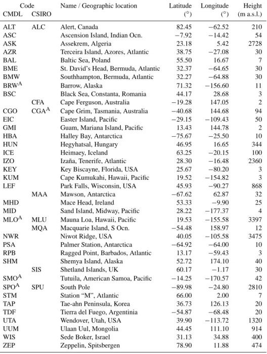
Table A1. List of measurement sites used.ASite where flask records have been replaced by in-situ records in assessment A.
Code Name / Geographic location Latitude Longitude Height
CMDL CSIRO (◦) (◦) (m a.s.l.)
ALT ALC Alert, Canada 82.45 −62.52 210
ASC Ascension Island, Indian Ocn. −7.92 −14.42 54
ASK Assekrem, Algeria 23.18 5.42 2728
AZR Terceira Island, Azores, Atlantic 38.75 −27.08 30
BAL Baltic Sea, Poland 55.50 16.67 7
BME St. David’s Head, Bermuda, Atlantic 32.37 −64.65 30
BMW Southhampton, Bermuda, Atlantic 32.27 −64.88 30
BRWA Barrow, Alaska 71.32 −156.60 11
BSC Black Sea, Constanta, Romania 44.17 28.68 3
CFA Cape Ferguson, Australia −19.28 147.05 2
CGO CGAA Cape Grim, Tasmania, Australia −40.68 144.68 94
EIC Easter Island, Pacific −29.15 −109.43 50
GMI Guam, Mariana Island, Pacific 13.43 144.78 2
HBA Halley Bay, Antarctica −75.67 −25.50 10
HUN Hegyhatsal, Hungary 46.95 16.65 344
ICE Heimaey, Iceland 63.25 −20.15 100
IZO Iza˜na, Tenerife, Atlantic 28.30 −16.48 2360
KEY Key Biscayne, Florida, USA 25.67 −80.20 3
KUM Cape Kumukahi, Hawaii, Pacific 19.52 −154.82 3
LEF Park Falls, Wisconsin, USA 45.93 −90.27 868
MAA Mawson, Antarctica −67.62 62.87 32
MHD Mace Head, Ireland 53.33 −9.90 25
MID Sand Island, Midway, Pacific 28.22 −177.37 4
MLOA MLU Mauna Loa, Hawaii, Pacific 19.53 −155.58 3397
MQA Macquarie Island, S Ocn. −54.48 158.97 12
NWR Niwot Ridge, USA 40.05 −105.58 3475
PSA Palmer Station, Antarctica −64.92 −64.00 10
RPB Ragged Point, Barbados, Atlantic 13.17 −59.43 3
SHM Shemya Island, Alaska 52.72 174.10 40
SIS Shetland Islands, UK 60.17 −1.17 30
SMOA Tutuila, American Samoa, Pacific −14.25 −170.57 42
SPOA SPU South Pole −89.98 −24.80 2810
STM Station “M”, Atlantic 66.00 2.00 7
TAP Tae-ahn Peninsula, Korea 36.73 126.13 20
TDF Tierra del Fuego, Argentinia −54.87 −68.48 20
UTA Wendover, Utah, USA 39.90 −113.72 1320
UUM Ulaan Uul, Mongolia 44.45 111.10 914
WIS Sede Boker, Israel 31.13 34.88 400
ZEP Zeppelin, Spitsbergen 78.90 11.88 474
Acknowledgements. Fruitful discussions with C. Le Qu´er´e,
P. Steele, K. Masarie, M. Gloor, C. Gerbig, and M. Heimann are gratefully acknowledged. Cape Grim in-situ data were provided by P. Steele and P. Krummel of CSIRO in collaboration with
the Australian Bureau of Meteorology. We are obliged to the
computing centers Deutsches Klimarechenzentrum Hamburg and Gesellschaft f¨ur wissenschaftliche Datenverarbeitung G¨ottingen for their kind support.
Edited by: W. E. Asher
References
Baker, D. F., Law, R. M., Gurney, K. R., Rayner, P., Peylin, P., Denning, A. S., Bousquet, P., Bruhwiler, L., Chen Y.-H., Ciais, P., Fung, I. Y., Heimann, M., John, J., Maki, T., Maksyutov, S., Masarie, K., Prather, M., Pak, B., Taguchi, S., and Zhu, Z.: TransCom3 inversion intercomparison: Interannual variabil-ity of regional CO2sources and sinks, 1988–2003, Global Bio-geochem. Cycles, 20, GB 1002, doi:10.1029/2004GB002439, 2006.
Bousquet, P., Peylin, P., Ciais, P., Le Qu´er´e, C., Friedlingstein, P., and Tans, P.: Regional changes in carbon dioxide fluxes of land
and oceans since 1980, Science, 290, 1342–1346, 2000. Churkina, G. and Trusilova, K.: A global version of the biome-bgc
terrestrial ecosystem model, Tech. Rep., Max Planck Institute for Biogeochemistry, Jena, 2002.
Conway, T., Tans, P., Waterman, L., Thoning, K., Kitzis, D., Masarie, K., and Zhang, N.: Evidence for interannual variabil-ity of the carbon cycle from the national oceanic and atmo-spheric administration climate monitoring and diagnostics labo-ratory global air sampling network, J. Geophys. Res., 99, 22 831– 22 855, 1994.
GLOBALVIEW-CO2: Cooperative Atmospheric Data Integration Project – Carbon Dioxide. CD-ROM, NOAA CMDL, Boulder, Colorado (also available on Internet via anonymous FTP to ftp: //ftp.cmdl.noaa.gov, Path: ccg/co2/GLOBALVIEW), 2004. Gloor, M., Gruber, N., Sarmiento, J., Sabine, C., Feely, R.,
and R¨odenbeck, C.: A first estimate of present and prein-dustrial air-sea CO2flux patterns based on ocean interior car-bon measurements and models, Geophys. Res. Lett., 30, 1010, doi:10.1029/2002GL015594, 2003.
Gurney, K., Law, R. M., Denning, A. S., et al.: Towards robust regional estimates of CO2sources and sinks using atmospheric transport models, Nature, 415, 626–630, 2002.
Francey, R. J., Steele, L. P., Spencer, D. A., Langenfelds, R. L., Law, R. M., Krummel, P. B., Fraser, P. J., Etheridge, D. M., Derek, N., Coram, S. A., Cooper, L. N., Allison, C. E., Porter, L., and Baly, S.: The CSIRO (Australia) measurement of greenhouse gases in the global atmosphere, report of the 11th WMO/IAEA Meeting of Experts on Carbon Dioxide Concentration and Related Tracer Measurement Techniques, Tokyo, Japan, September 2001, edited by: Toru, S. and Kazuto, S., World Meteorological Organization Global Atmosphere Watch, 97–111, 2003.
Masarie, K., Langenfelds, R., Allison, C., Conway, T., Dlugo-kencky, E., Francey, R., Novelli, P., Steele, L., Tans, P., Vaughn, B., and White, J.: NOAA/CSIRO flask air intercomparison ex-periment: A strategy for directly assessing consistency among atmospheric measurements made by independent laboratories, J. Geophys. Res., 106, 445–464, 2001a.
Masarie, K., Tans, P., and Conway, T.: GLOBALVIEW-CO2: Past, present and future, in: Report of the eleventh WMO/IAEA meet-ing of experts on carbon dioxide concentration and related tracer measurement techniques, edited by: Toru, S. and Kazuto, S., Tokyo, 2001b.
Olivier, J. G. J. and Berdowski, J. J. M.: Global emissions sources and sinks, in: The Climate System, edited by: Berdowski, J., Guicherit, R., and Heij, B. J., A. A. Balkema Publishers/Swets & Zeitlinger Publishers, Lisse, The Netherlands, ISBN 90 5809 255 0, 33–78, 2001.
Peylin, P., Bousquet, P., Le Qu´er´e, C., Sitch, S., Friedling-stein, P., McKinley, G., Gruber, N., Rayner, P., and Ciais, P.: Multiple constraints on regional CO2 flux variations over land and oceans, Global Biogeochem. Cycles, 19, GB 1011, doi:10.1029/2003GB002214, 2005.
Rayner, P., Enting, I., Francey, R., and Langenfelds, R.: Recon-structing the recent carbon cycle from atmospheric CO2, δ13CO2 and O2/N2observations, Tellus B, 51, 213–232, 1999.
R¨odenbeck, C., Houweling, S., Gloor, M., and Heimann, M.: CO2 flux history 1982–2001 inferred from atmospheric data using a global inversion of atmospheric transport, Atmos. Chem. Phys., 3, 1919–1964, 2003,
SRef-ID: 1680-7324/acp/2003-3-1919.
R¨odenbeck, C.: Estimating CO2 sources and sinks from
at-mospheric mixing ratio measurements using a global
inversion of atmospheric transport, Technical Report
6, Max Planck Institute for Biogeochemistry, Jena,
http://www.bgc-jena.mpg.de/mpg/websiteBiogeochemie/ Publikationen/Technical Reports/tech report6.pdf, 2005. Steele, L. P., Krummel, P. B., Spencer, D. A., Porter, L. W., Baly,
S. B., Langenfelds, R. L., Cooper, L. N., van der Schoot, M. V., and Da Costa, G. A.: Baseline carbon dioxide monitoring, in: Baseline Atmospheric Program (Australia) 2001–2002, edited by: Cainey, J. M., Derek, N., and Krummel, P. B., Bureau of Me-teorology and CSIRO Atmospheric Research, Melbourne, Aus-tralia, 36–40, 2004.
Takahashi, T., Sutherland, S. C., Sweeney, C., Poisson, A., Metzl, N., Tilbrook, B., Bates, N., Wanninkhof, R., Feely, R. A., Sabine, C., Olafsson, J., and Nojiri, Y.: Global sea-air CO2flux based on climatological surface ocean pCO2, and seasonal biological and temperature effects, Deep Sea Res. II, 49, 1601–1623, 2002. Tans, P. P., Thoning, K. W., Elliott, W. P., and Conway, T. J.: Error
estimates of background atmospheric CO2patterns from weekly flask samples, J. Geophys. Res., 95, 14 063–14 070, 1990. Zhao, C.L., Tans, P. P., and Thoning, K. W.: A high precision
mano-metric system for absolute calibrations of CO2in dry air, J. Geo-phys. Res., 102, 5885–5894, 1997.