Design of a stabilization method for cable suspended camera systems

(1)

Design of a Stabilization Method for Cable Suspended Camera Systems

by

Nicolas Arons

Submitted to the

Department of Mechanical Engineering

in Partial Fulfillment of the Requirements for the Degree of Bachelor of Science in Mechanical Engineering

at the

Massachusetts Institute of Technology

May 2020

Signature of Author:

Department of Mechanical Engineering May 1, 2020

Certified by:

David Trumper Professor of Mechanical Engineering Thesis Supervisor

Accepted by:

(2)

(3)

Design of a Stabilization Method for Cable Suspended Camera Systems

by

Nicolas Arons

Submitted to the Department of Mechanical Engineering on May 1, 2020 in Partial Fulfillment of the

Requirements for the Degree of

Bachelor of Science in Mechanical Engineering

ABSTRACT

Scootah Hockey is a small sport with a yearly championship held in Simmons Hall at MIT. To help grow the sport, a cable suspended camera system called the SHKYCAM was designed to enable online streaming of matches. Due to unique features of the sport, the SHKYCAM encounters large disturbances during the normal course of play, resulting in shaky video footage and a poor streaming experience. In this thesis, a literature study of cable mounted camera systems was performed to understand current solutions used in camera stabilization during sporting events. Additionally, a controller was designed to be used with a flywheel to steady the system in response to a disturbance. In simulation, the controller reduced the settling time by four orders of magnitude, but was ultimately deemed infeasible to implement.

Thesis Supervisor: David Trumper

(4)

List of Figures

Figure 1: Footage from the 2018 Scootah Hockey World Championship tournament 7

Figure 2: CAD Rendering of the SHKYCAM 8

Figure 3: One anchor point for the SHKYCAM 8

Figure 4: Pendulum model of the SHKYCAM 10

Figure 5: Block Diagram for the pendulum model with feedback control 11

Figure 6: Circuit diagram for the motor 11

Figure 7: Block diagram for the motor 12

Figure 8: Bode plot for the combined motor and pendulum plant 13

Figure 9: Bode plot of the return ratio 15

Figure 10: Pendulum’s response to a torque impulse input 16

Figure 11: The closed loop system’s response to a torque impulse input 17 Figure 12: Bode plot of the Sensitivity of the closed loop system 18

(6)

List of Tables

(7)

1. Introduction

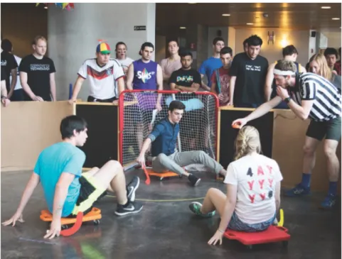
Scootah Hockey is a small but growing sport that was started in Simmons Hall at MIT. It consists of two teams of three people each, sitting on plastic, elementary-gym style scooters hitting a puck around with plastic sticks, trying to score in the opposite team’s goal. Although new, having started officially in 2015, the sport has grown to over 110 competitors and over 180 spectators at last year’s event. Figure 1 shows a picture from the 2018 Scootah Hockey World Championships, held in Simmons Hall at MIT.

Figure 1: Footage from the 2018 Scootah Hockey World Championship tournament. Players, with teams denoted by differently colored sticks, are shown on their scooters, with the referee ready to drop the puck into play.

Due to the sport’s growth, an attempt was made to reach a larger audience through streaming the event online. To create a better viewing experience for the online audience, a prototype cable mounted camera, named the SHKYCAM (Scootah Hockey Kable Y’nabled Camera Action Machine). Seen in Figure 2, the SHKYCAM consists of a driving motor and pulley, two balancing pulleys, pan and tilt servos for the camera, and a metal frame to hold it together and for electronics to be mounted.

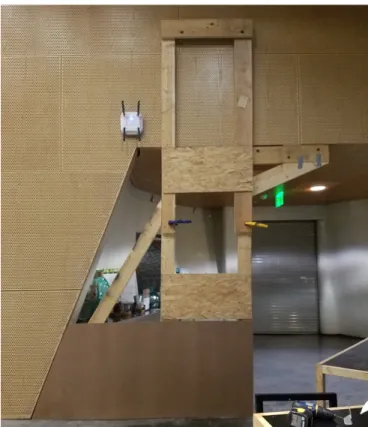
On one end of the mounting rope, the SHKYCAM was connected rigidly to metal structural supports inside the Simmons Dining hall. The other end of the mounting rope is connected to a free standing wooden construction. Seen in Figure 3, this also functions as a wall for the game. Players often push off of the wall with their feet, leading to vibrations in the

structure and consequently the rope, which translate to the camera and causes the video stream to become poor. Because of this, a method for stabilizing the SHKYCAM was investigated as a way to increase the quality of the video stream.

(8)

Figure 2: A CAD Rendering of the SHKYCAM. The motor, pulleys and aluminum body are present, while the electronics, pan and tilt motors, and camera are not shown.

Figure 3: One anchor point for the SHKYCAM whose lower half doubles as in-game wall. Players often kick against this wall during games, which leads to large disturbances on the

(9)

2. Background

There are a number of patents related to aerial cable-mounted camera systems which proved helpful in analyzing and understanding the SHKYCAM.

One patent, “Aerial Camera System,” U.S. number 8,199,197 B2, used a quite complex system for controlling and stabilizing the image from their cable mounted camera system [1]. This particular patent has the camera move in three dimensions (as opposed to just one for the SHKYCAM) by utilizing four motors in corners of a stadium, for example [1]. This particular patent was used in the Skycam © which is used in major sporting events including football, soccer and the Olympics, all around the world. This patent described a method for stabilizing the camera, using a passive flywheel system as well as an active motor control [1]. There are two flywheels positioned perpendicularly to each other with their angular momentum vectors parallel to the plane of the ground [1]. Spinning at high speed, these flywheels add to the effective inertia of the system and help stop high frequency torque disturbances in the two directions

perpendicular to their momentum vectors [1]. The actively controlled motors are the solution for the lower frequency, longer term disturbances as they correct for angle based on an

accelerometer measuring the angle of the system. On top of this, the system has pan and tilt motors for the camera that run control loops for keeping the camera even more stable based on accelerometers on the camera [1]. All of this helps to ensure the incredibly clear image that millions of people have viewed on their televisions.

While the ingenuity of this patent is quite impressive, the same ideas cannot be applied directly to the SHKYCAM. One limitation the SHKYCAM has is cost; the budget of Simmons Hall is much less than the budget of a professional sports team, and so sacrifices in quality will have to be made. Additionally, due to the constraints of the stadium in which the SHKYCAM is mounted, it cannot have the four-wire system of this patent. Not all four corners of the Simmons Dining Hall have secure anchor points, and forcing such a design on a constrained space could result in accident or injury. Similarly, due to the constraints posed by the anchor points for the SHKYCAM, the weight of the system needs to be much less.

U.S. Patent number 5,784,966, named “Stabilized Lightweight Equipment Transport System”, is a design for equipment, potentially a camera, to be transported over a rail at high speeds while keeping the camera relatively stabilized [2]. This patent’s main goal is to “provide a lightweight, track mounted equipment trans porting system that is isolated from the minute vibrations inherent in existing rail system and stabilized without resort to heavy mass/gyro-systems” [2]. It acknowledges the mass issues of complete gyro-systems, as seen with the first patent [2]. However, it differs from the SHKYCAM in two main ways: the rail mounted nature of the system doesn’t have the inherent compliance that a cable mounted system does; they assume the vibrations affecting the camera are minute. Due to the naturally high compliance of rope and wires as compared to stiff rails, any force transmitted on the rope will result in much bigger resultant oscillations at the camera than if the camera were mounted on a rail.

Additionally, the SHKYCAM environment is not inherently free of disturbances. As mentioned earlier, one of the anchor points doubles as a wall for the game, causing players to push off it with their feet and occasionally slide into it on their scooters.

(10)

This patent is also referenced in “Cable Camera Systems And Methods”, U.S. patent number 9,154,673 B2 [3]. Figure 1 of this patent has an incredibly similar architecture to the currently designed SHKYCAM, seen above [3]. This validates the SHKYCAM’s 3 pulley drive system and the pan and tilt motor-controlled axis supporting a camera. This patent, however, fails to mention any stabilization methods for the camera, only writing that stabilization equipment can be added [3].

3. Controller Design

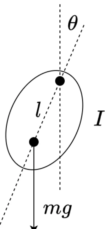
To address the video quality issues with the current SHKYCAM design, control through spinning flywheel along the axis of the rope was considered. In modeling the system, it was sufficient to treat the SHKYCAM as a body swinging from a fixed point. Figure 4 shows the model.

Figure 4: Pendulum model of the SHKYCAM. The angle 𝜃 measures rotation from vertical. The body has rotational inertia 𝐼 and mass 𝑚 a distance 𝑙 from the pivot point. Gravity 𝑔 acts downwards.

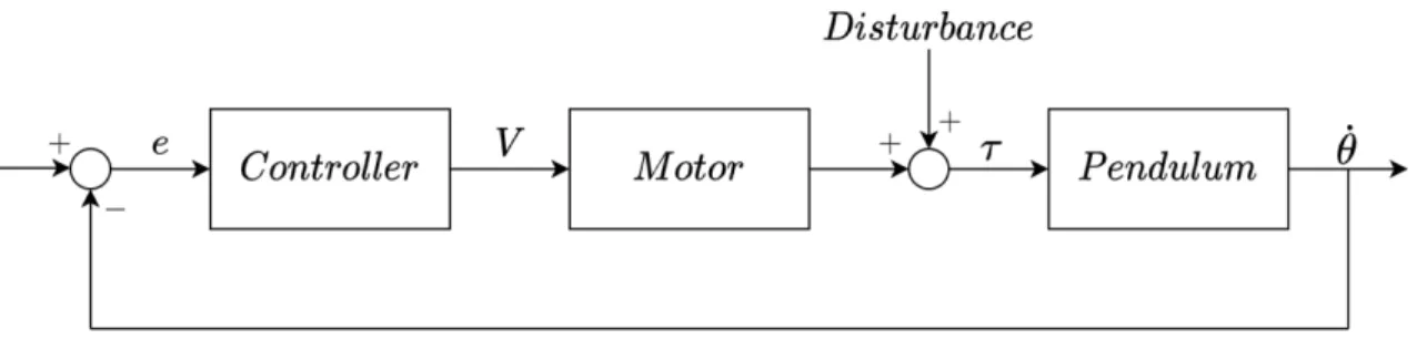
3.1 Block Diagram

A Block diagram was constructed to aid in analysis. Figure 5 shows the block diagram. The reference 𝑟 is set to 0 and the speed of the pendulum 𝜃̇ is controlled and measured using a gyroscope. The disturbance is modeled as an external torque applied to the pendulum.

(11)

Figure 5: Block Diagram for the pendulum model with feedback control.

In order to use classical controls to analyze this system, the dynamics of the pendulum must be linearized. The dynamics of the pendulum are given in equation (1):

𝜏 = 𝐼𝜃̈ + 𝐶𝜃̇ + sin 𝜃 𝑚𝑔𝑙 (1)

Linearizing about 𝜃 = 0 makes sense due it being the pendulum’s natural point of stability. At this point, the approximation 𝑠𝑖𝑛(𝜃) = 𝜃 is accurate within 0.3% for 𝜃 up to 15 degrees or 0.26 radians. The linearized dynamics are shown in equation (2):

𝜏 = 𝐼𝜃̈ + 𝐶𝜃̇ + 𝜃𝑚𝑔𝑙 (2)

Applying the Laplace transform to the linearized dynamics and solving for 𝜃̇/𝜏. gives us our pendulum transfer function in equation (3):

𝜃̇(𝑠) 𝜏(𝑠) = 1 𝐼 𝑠 𝑠:₊𝐶 𝐼 𝑠 +𝑚𝑔𝑙𝐼 (3)

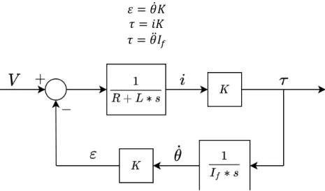
Motor transfer function for torque/velocity: The dynamics of the motor are derived from the motor’s electrical circuit, shown in Figure 6.

Figure 6: The circuit diagram for the motor. The resistance 𝑅 and the inductance 𝐿 are in series with the back emf 𝜀 and the input voltage 𝑉_?@.

Combing an analysis of the motor’s circuit with equations (4), (5) and (6) give us the block diagram for the motor, shown in Figure 7 below. Equation (4) shows the relationship between speed and back EMF using the motor constant 𝐾, equation (5) shows the relationship between current 𝑖 and torque 𝜏 𝑢𝑠𝑖𝑛𝑔 𝐾, and equation (6) shows the relationship between angular acceleration 𝜃̈ and torque using the flywheel’s inertia 𝐼 .

(12)

𝜀 = 𝜃̇𝐾 (4)

𝜏 = 𝑖𝐾 (5)

𝜏 = 𝜃̈𝐼_C (6)

Figure 7: Block diagram for the motor. Voltage V is input with an output torque 𝜏. The intermediate variables include the current 𝑖, the back emf 𝜀, and the motor speed 𝜃̇. Applying Black’s formula to this block diagram reveals the motor’s transfer function:

𝜏(𝑠) 𝑉(𝑠)= 𝐾 𝐿 𝑠 𝑠: + 𝑅𝐿 𝑠 +𝐿𝐼𝐾:_C (7)

The characteristic time constant for the motor circuit is given by 𝜏 = 𝐿/𝑅. If this value is sufficiently small, the motor’s transfer function can be simplified to equation (8) below. This assumption holds valid for the specific analysis later, as the motor’s electrical dynamics are two orders of magnitude faster than the closed loop dynamics.

𝜏(𝑠) 𝑉(𝑠)= 𝐼_C 𝐾 𝑠 𝐼_C𝑅 𝐾: 𝑠 + 1 (8)

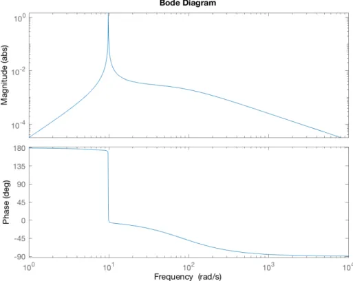
Combining the motor and the pendulum’s transfer function the overall plant’s transfer function, 𝜃̈/𝑉. The bode plot for this transfer function is show in Figure 8.

(13)

Figure 8: Bode plot for the combined motor and pendulum plant. The sharp peak is characteristic of an underdamped system.

3.2 Parameter Values

The values used for designing and evaluating the controller were chosen to represent the system. While some parameters were well known, others such as the motor constant and

resistance were estimated based on reasonable values.

Table 1: The parameter values used in controller design. The values were estimated to best represent the system with the knowledge available.

Parameter Name Value

𝑚 Mass of SHKYCAM 1.4 𝑘𝑔

𝑙 Distance from Center of Mass to pivot point on rope 0.1 𝑚 𝐼 Rotational inertia of SHKYCAM about pivot 0.014𝑘𝑔𝑚:

𝐾 Motor Constant 0.0987 𝑁𝑚/𝐴

𝑅 Motor Resistance 3 Ω

𝐼C Inertia of flywheel 0.00035𝑘𝑔𝑚:

𝐿 Motor Inductance 100 𝜇𝐻

(14)

3.3 Controller Specifications

The desired bandwidth for the closed loop was 300 rad/s. This was chosen based on both the constraints of the problem and the desired response characteristics. Inertial measurement units (IMU’s) often have their sampling frequency set at 1.6kHz, or 10,000 rad/s. In order to use the continuous time approximation of this discrete time system, the crossover frequency for our return ratio should be 30 times less than the sampling frequency, leading to a maximum

crossover of 333 rad/s, above our designed 300 rad/s. For many cameras, video is captured at 30 frames per second, which translates to 0.033 seconds per frame. As shown later, the designed controller is able to reach its settling time in response to a disturbance in a little over 0.033 seconds. This means that it can effectively stop the velocity of the camera in one frame. With the chosen parameters, the 𝐿/𝑅 time constant of the motor leads to a frequency of 30,000 rad/s, two decades above our crossover. This verifies the assumption that the circuit dynamics are

sufficiently fast to ignore them.

3.4 Controller Architecture

To achieve the desired 300 rad/s bandwidth, the controller was designed with an integrator, a double lag compensator, a lead compensator, and a proportional gain.

The general form of a lag compensator is given by equation (9), with 𝑎 being the location of the zero and 𝑏 the location of the pole. The lag compensators were picked to have 𝑏 equal to 0 to have their poles at the origin to offset the plant’s zeros there. The zeros were chose such that 𝑎 was equal to 30, corresponding to a break point approximately one decade above crossover. This means that the lag compensator will have a small effect (5.7 degrees each) on phase margin (and hence stability), but they still maintain a relatively fast response for the characteristic “long tail” of the lag compensator.

𝐿𝑎𝑔(𝑠) =𝑠 + 𝑎 𝑠 + 𝑏

(9)

The lead compensator transfer function is given by equation (10). By setting 𝜔 equal to your crossover frequency, you can add phase at crossover by arcsin(𝛼 − 1)/(𝛼 + 1). For the lead compensator design, it was centered around crossover at 316 rad/s with an alpha=10 to allow for a 54.9 degree phase boost near crossover. Because of the integrator and the plant’s poles, having one lead compensator still allowed for a -2 slope at crossover, ensuring a well-defined crossover frequency. The proportional gain was chosen such that the desired crossover frequency had magnitude 1, thus ensuring that it was the crossover point. This value turned out to be 390000. The final transfer function for the controller is given by equation (11).

𝐿𝑒𝑎𝑑(𝑠) = √𝛼𝑠 + 𝜔/√𝛼 𝑠 + 𝜔√𝛼

(10)

(15)

4. Results and Discussion

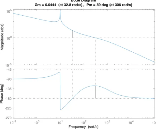
4.1 Return Ratio

Figure 9 shows the return ratio, which has a well-defined crossover at 306 rad/s, very close to the 300 rad/s goal. Additionally, the 59 degrees of phase margin is very good for stability of the system.

Figure 9: Bode plot of the return ratio 𝐿(𝑠) = 𝐶𝑜𝑛𝑡𝑟𝑜𝑙𝑙𝑒𝑟 ⋅ 𝑀𝑜𝑡𝑜𝑡 ⋅ 𝑃𝑒𝑛𝑑𝑢𝑙𝑢𝑚. The crossover frequency happens at 306 rad/s, which is very close to the designed 300 rad/s.

4.2 Disturbance rejection

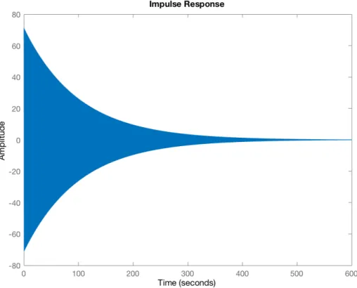
As seen in the block diagram, a disturbance to the system was modeled as a torque. An impulse was chosen as the input function, as it best characterized the high force, small time impacts that a person running into the base of the cable support would cause.

For the pendulum without any control, the system’s stability comes from the damping 𝐶. Because this value is so small, the pendulum takes nearly 400 seconds to some within 2% settling. Figure 10 shows the pendulum’s response to a torque impulse input.

(16)

Figure 10: Pendulum’s response to a torque impulse input. The solid body indicates many unseen oscillations due to the long time scale on which the decay happens.

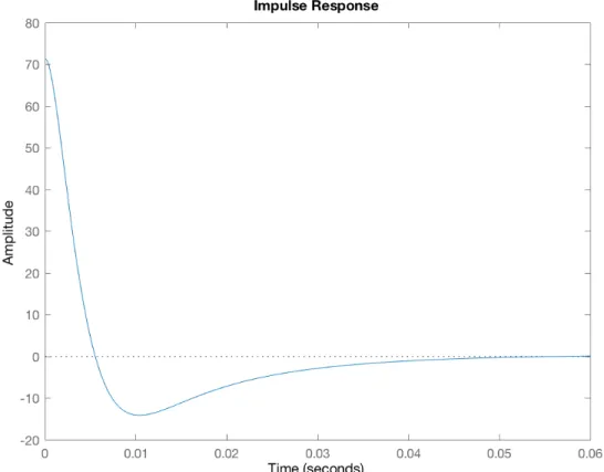
When we apply our controller and add feedback, the system’s performance improves vastly. The velocity of the system quickly slows, settling to within 2% in 0.0373 sec, or just over one camera frame. Figure 11 shows the time response of the closed loop system to an impulse disturbance input.

(17)

Figure 11: The closed loop system’s response to a torque impulse input. The system settles very quickly, especially compared to the case without control.

4.3 Sensitivity

The sensitivity of a closed loop system is computed through the following transfer function, where 𝐿(𝑠) is the return ratio.

𝑆 = _{1 + 𝐿(𝑠)}1 (12)

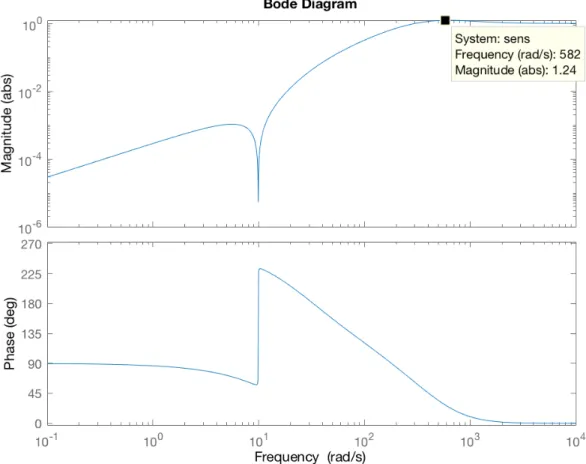
Figure 12, the bode plot for the sensitivity of the closed loop system, shows a maximum sensitivity value of 1.24. This implies that the system is very stable and that small changes in the dynamics of the system, like a change in inertia due to a camera being panned, will not change the stability and effectiveness of this controller.

(18)

Figure 12: Bode plot of the Sensitivity of the closed loop system. The max value, as indicated on the plot, is 1.24.

4.4 Implementation Issues

While the controller was not implemented on a real system due to the limited scope of this thesis, there are problems with the proposed controller’s practicality. Due to the controller’s poles at the origin, the control effort will be unbounded, resulting in an infinite voltage output for a finite disturbance input. For this reason, this controller is infeasible and not recommended, and other designs should be considered.

5. Conclusions

The literature review proved helpful in identifying ways in which other similar systems control and stabilize their cameras, both actively and passively. Although none apply directly to the SHKYCAM due to its unique set of restrictions and constraints, the design process and thinking that was present in the patents will help the author in future iterations of the SHKYCAM.

(19)

needed, necessitating the use of discrete controller design methods. Additionally, all of the parameters of the pendulum and motor are estimations and subject to change. The proposed controller also has implementation issues discussed earlier. However, the success of the

controller in disturbance rejection points to the promise of feedback control as a way to stabilize the video feed even in the high disturbance environment that is a Scootah Hockey match.

6. References

[1] Bennett, P. J., Cook, G., Jones, M. R., Ashenayi, K., Henry, M. F., and MacDonald, A., 2018, “Aerial Camera System.”

[2] Brown, G. W., and Keller, D., 1998, “Stabilized Lightweight Equipment Transport System.” [3] Stone, K., 2015, “Cable Camera Systems and Methods.”