HAL Id: hal-00004638
https://hal.archives-ouvertes.fr/hal-00004638v2
Preprint submitted on 22 Mar 2006HAL is a multi-disciplinary open access
archive for the deposit and dissemination of sci-entific research documents, whether they are pub-lished or not. The documents may come from teaching and research institutions in France or abroad, or from public or private research centers.
L’archive ouverte pluridisciplinaire HAL, est destinée au dépôt et à la diffusion de documents scientifiques de niveau recherche, publiés ou non, émanant des établissements d’enseignement et de recherche français ou étrangers, des laboratoires publics ou privés.
Continuity of the trace operator with respect to the
domain and application to shape optimization
A. Boulkhemair, A. Chakib, A. Nachaoui
To cite this version:
A. Boulkhemair, A. Chakib, A. Nachaoui. Continuity of the trace operator with respect to the domain and application to shape optimization. 2006. �hal-00004638v2�
Continuity of the trace operator with respect to the domain and
application to shape optimization
A. Boulkhemair1, A. Chakib2 and A. Nachaoui1
1 Laboratoire de Math´ematiques Jean Leray,
CNRS UMR6629/ Universit´e de Nantes,
2, rue de la Houssini`ere, BP 92208, 44322 Nantes, France.
E-mail: boulkhem@math.univ-nantes.fr & nachaoui@math.univ-nantes.fr
2 D´epartement de Math´ematiques Appliqu´ees et Informatique
FST de Beni-Mellal, Universit´e Cadi-Ayyad B.P. 523, Beni-Mellal, Morocco.
E-mail: chakib@fstbm.ac.ma
Abstract
Shape optimization amounts to find the optimal shape of a domain which minimizes a given criterion, often called a cost functional. Here, we are interested in the case where the criterion is computed through the solution of a partial differential equation, the so-called state equation, which makes the optimization problem non-trivial. We use a general parameterization of the unknown boundary in order to preserve the physical general information and we prove the continuity of the cost functional.
1
Introduction
Varying domains constitute an important type of inverse problems which appear in connection with a variety of phenomenon in different fields. Shape Identification, free or moving boundary problems, phase change or elastic contact problems fall into the class of such inverse problems with a priory unknown domains. Some problems that lead to boundary inverse problems are: the dam seepage problem [14]; Riabouchinsky flow past circular disks [21]; Falling droplets [35, 32, 38]; the Alt-Caffarelli or Bernoulli problem [4]. The common structure of these problems is that there are elliptic equations for m unknowns and m + 1 mixed Dirichlet-Neumann conditions on the unknown surface. Many more problems also fall into this general category, with applications to aluminium production by electrolytic reduction [13]; groundwater flow [25, 29]; free surface waves [9]]; semiconductors [2, 16]; electromagnetic casting [33, 31]; the Dam and Bernoulli problems [10, 37, 28, 22, 17].
There is no previous analytic theory covering this general class of boundary inverse problems, although there has been progress on individual problems.
A variety of techniques exist for numerically solving boundary inverse problems, see [14, 26, 16, 1, 11] and the references therein. Among this, shape optimization technique is a useful method for solving the type of problems mentioned above. This is a variational approach, minimizing an integral functional over the variable domain having an unknown boundary. For an introduction to shape optimization, cf [23, 36] and some examples of its use are given in [5, 8, 15, 18, 34].
A general formulation of such optimal shape approaches can be expressed as follows
(
Minimize J(Ω, u)
subject to Ω ∈ Θad and u ∈ U(Ω),
(1) where U(Ω) denotes the set of solutions of a given partial differential equation on the domain Ω (state equation on Ω) and Θad is a set of admissible domains.
In order to show the existence of a solution for this type of problems, a widely used method is to show that the space F = {(Ω, u) , Ω ∈ Θad, u ∈ U(Ω)} is compact with a suitable topology on
F which is induced from topologies on Θad and U(Ω), and that the cost functional J is lower semi
continuous on F [23].
In this paper, we are interested in the continuity of cost functionals that can be associated to the determination of the location, size and shape of an unknown portion Γ, of the boundary ∂Ω of a domain Ω ⊂R2, from given, Dirichlet and Neumann, boundary conditions on this unknown part of the boundary. More precisely, we consider the boundary cost functional J defined by
J(Ω, u) =
Z
Γ(u − g)
2dσ, which is associated with problems where a condition of the type u = g has
to be imposed on Γ. The function g is given and u is the solution of a partial differential equation on Ω. In the case where the unknown boundary Γ is the graph of a function, continuity results for this type of functionals with a suitable topology on F have been obtained in [6, 10, 24]. However, in many physical problems this assumption on the unknown boundary is too restrictive. The situation where the unknown boundary can not be the graph of a function occurs in many engineering problems such as, for example, the dam problem in non-homogeneous porous media [10, 19, 22], the Stefan problem [20], optimal insulating and electro-chemistry [3, 17] and the semiconductor problem [27, 16]. Here, we use a general parameterization of the unknown boundary in order to preserve the physical general information on this boundary. The topology we use on Θad is just
that associated to the C1 convergence of the parameterizations.
The main result of this paper is the continuity of the trace operator from Hr(Ω) (1 ≥ r > 1 2)
to L2(Γ) with a constant independent of Γ. This is proved in section 3. At this stage, it should be
noted that, in the case of a family of domains with parallel boundaries, a similar result has been obtained by Lions and Magenes in [30]. The continuity of the cost functional J on the space F is established in section 4. Actually, we prove the continuity of a more general functional.
2
Notations and definitions
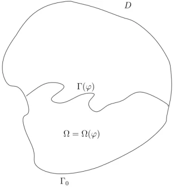
Let D be a fixed C1 open connected bounded subset of R2. An admissible domain Ω will be an
open subset of D. The boundary ∂Ω of Ω is assumed to consist in two parts ∂Ω = Γ0∪ Γ such that
Γ0∩ Γ = ∅, meas(Γ0) > 0 and meas(Γ) > 0, where Γ is the free boundary part defined by Γ = Γ(ϕ) = {ϕ(t) = (ϕ1(t), ϕ2(t)) ; t ∈ [0, 1]},
ϕ : [0, 1] →R2 is a parameterisation and Γ is assumed to have its endpoints on the boundary of D (see figure 1). In fact, in this general setting, the curve Γ(ϕ) can divide D into two open subsets. This is the case for example when D is simply connected. We have then to choose Ω. We can make for example the following choice : We follow the natural orientation given by the parameterisation and take the open set whose exterior unit normal boundary vector is on the left.
We shall also write Ω = Ω(ϕ) to indicate the dependence on the parameterization ϕ.
Ω = Ω(ϕ)
Γ0
Γ(ϕ)
D
Figure 1: An example of the considered domain Ω = Ω(ϕ). We shall denote by ν(x) the exterior unit normal vector to ∂D at x ∈ ∂D. Define Vadto be the set of vector functions ϕ ∈ C1
¡
[0, 1],R2¢satisfying the following conditions :
|ϕ(t)| ≤ C0, ∀t ∈ [0, 1],
C1|t − t0| ≤ |ϕ(t) − ϕ(t0)| ≤ C2|t − t0|, ∀t, t0∈ [0, 1],
ϕ([0, 1]) ⊂ D and, for t = 0 or 1, ϕ(t) ∈ ∂D,
for t = 0 or 1, |ν(ϕ(t)).ϕ0(t)| ≥ ²0, (2) and, for all t ∈ [0, 1], d(ϕ(t), ∂D) ≥ ²1t(1 − t), (3)
where C0, C1, C2, ²0and ²1are positive fixed constants, d(ϕ(t), ∂D) is the distance of the point ϕ(t)
from the boundary ∂D, and we are using the standard notations |(a, b)| =√a2+ b2, (a, b).(a0, b0) =
aa0+ bb0. Note that the assumptions (2) and (3) are made to insure that the curve Γ(ϕ) touches the
boundary ∂D only two times (with the endpoints) and in a transverse manner. The consequence of this is that the domain Ω(ϕ) is Lipschitz regular.
Now, the set Uad of admissible functions will be any compact subset of Vad. In other words,
Uad is a subset of Vad whose elements and their derivatives are equicontinuous as it follows from
Ascoli-Arzel`a theorem. An example of such a set Uad is that of a closed subset of Vad which is bounded in C1,δ¡[0, 1] ,R2¢ for some δ such that 0 < δ ≤ 1.
The space of admissible domains is then defined by :
Θad= {Ω = Ω(ϕ) ⊂ D ; ϕ ∈ Uad} .
Note that the elements of Θad are uniformly Lipschitz open sets of R2 and so they satisfy the
uniform cone property [34].
Assume that u = u(Ω) ∈ H1(Ω) is the solution of a well posed problem such as
(
LΩu = f in Ω
L∂Ωu = h on ∂Ω,
(4)
where Ω ∈ Θad and LΩ and L∂Ω are partial differential operators on Ω and ∂Ω respectively.
The cost functional J we are interested in is then defined on the set
F = {(Ω(ϕ), u(Ω)) ; Ω(ϕ) ∈ Θad and u(Ω) solves (4) on Ω(ϕ)}
by
J(Ω(ϕ), u(Ω)) =
Z
Γ(ϕ)(u(Ω) − g) 2dσ,
where g is a given function on D having essentially the same regularity as u(Ω). For simplicity and without any restriction on our study, we shall assume that g = 0.
Now, the customary problem of shape optimization or optimal shape design is
to minimize J(Ω, u) on F. (5)
As we have already said, this minimization problem is usually solved by endowing the set F with a topology for which F is compact and J is lower semi-continuous. Let us therefore define the topology we shall work with. First, we define the convergence of a sequence (ϕn)n⊂ Uad by
ϕn −→ ϕ ⇐⇒
(
ϕn−→ ϕ uniformly on [0, 1]
ϕ0n−→ ϕ0 uniformly on [0, 1] (6) that is, iff ϕn → ϕ in the C1 topology. Then, the convergence of a sequence (Ω
n)n ⊂ Θad, such
that Ωn= Ω(ϕn), to Ω = Ω(ϕ) ∈ Θad is simply defined by
Ωn −→ Ω ⇐⇒ ϕn −→ ϕ. (7)
Denote byu the uniform extension of u from Ω to an open smooth bounded domain B (a disc, fore
example), such that D ⊂ B (see [12]). We define the convergence of a sequence (un)n of solutions
of (4) on Ω(ϕn) to u the solution of (4) on Ω(ϕ) by
Finally, the topology we put on F is the one induced by the convergence defined by (Ωn, un) −→ (Ω, u) ⇐⇒ ( Ωn−→ Ω un−→ u. (9) Thus, the compactness of F with respect to this topology depends on the type of the state problem (4) and on the compactness of Θad with respect to the convergence (7). At this stage, we have to
say that it is not our objective here to prove the compactness of F, the setting being too general. But since Uad is compact, one can obtain the compactness of F from the continuity of the state problem (4), which is based on the following (reasonable) condition : There exists a constant C > 0 such that ku(Ω)k1,Ω ≤ C, ∀Ω ∈ Θad. Anyhow, the chosen topology is rather natural, is used in
many applied problems and, as we shall see, it allows to prove the continuity of the cost functional
J and even the continuity of more general boundary functionals (see section 4).
3
Continuity of the trace operator
In this section, we give a proof of the trace theorem which allows us to estimate the norm of the trace operator by a constant independent of the free boundary Γ.
Theorem 1 Let u be in Hr(B), 1 ≥ r > 1
2, and Ω(ϕ) ∈ Θad. Then, there exists a constant K
independent of ϕ such that
kuk0,Γ(ϕ) ≤ K kukr,B
where k · k0,Γ(ϕ) is the L2(Γ(ϕ))-norm and k · k
r,B is the Hr(B)-norm.
The proof of this result is based on the following constructions and techniques.
Let ϕ ∈ Uad. By using standard techniques, we can construct a continuous extension operator
from C1¡[0, 1] ,R2¢ to ˜C1¡[−1, 2] ,R2¢ = {ϕ ∈ C1¡R,R2¢; supp(ϕ) ⊂ [−1, 2]}, such that the
extensionϕ of ϕ toe Rsatisfies
kϕe0kL∞(R)= kϕ0kL∞([0,1]), (10)
where k · kL∞ is the L∞-norm.
Now, let χ ∈ D(R) such that χ ≥ 0,
Z
R
χ dx = 1 and supp(χ) ⊂ [−1, 1]. We define the function ψk = (ψ1,k, ψ2,k), k ∈N∗, on Ras a regularized function ofϕ, that is,e
ψk(t) = Z R e ϕ(t − τ ) χ(kτ ) k dτ. Note that ψk0(t) = Z R e ϕ0(t − τ ) χ(kτ ) k dτ. Since ϕe0 is continuous, it is well known that ψ0
k converges uniformly to ϕe0 on any compact subset
ofR as k −→ ∞. In particular,
lim
k−→∞kψ 0
k− ϕ0kL∞([0,1])= 0.
In fact, we can show that for any ε > 0, there exists kε∈N∗independent of ϕ such that, for k ≥ kε,
Indeed, we have |ψk0(t) −ϕe0(t)| = | Z R ¡ e ϕ0(t − τ ) −ϕe0(t)¢ χ(kτ ) k dτ | ≤ Z R |ϕe0(t −τ k) −ϕe 0(t)| χ(τ ) dτ.
Since the extension operator is continuous from C1¡[0, 1] ,R2¢ to Ce1¡[−1, 2] ,R2¢, the functions e
ϕ0, are equicontinuous and uniformly continuous when ϕ describes U
ad. So, for ε > 0, there exists
γε> 0 independent of ϕ such that
∀t, t0∈R, |t − t0| ≤ γε implies that |ϕe0(t) −ϕe0(t0)| ≤ ε, ∀ϕ ∈ Uad. (11)
Hence, for k such that |τ |
k ≤ 1 k ≤ γε and all t ∈R, |ψk0(t) −ϕe0(t)| ≤ Z R ε χ(τ ) dτ = ε.
So, we can take kε= [γ1
ε] + 1, where [ · ] denotes the integral part.
Now, to the given ϕ ∈ Uad, we associate the function Φ ∈ C1¡[0, 1] ×R,R2¢defined by
Φ(t, s) = ϕ(t) + s ψk0ε(t)⊥, s ∈R, (12) where we are using the notation (a, b)⊥= (−b, a). In what follows, we shall omit the index k
ε and
write ψ instead of ψkε.
The following lemma is basic for the proof of Theorem 1.
Lemma 1 There exists a small enough s0 > 0 such that s0 is independent of ϕ ∈ Uad and the
following three assertions hold.
(i) The Jacobian, JΦ, of Φ is such that
|JΦ| ≥ 1
2C
2
1 on [0, 1] × [−s0, s0] . (13)
(ii) There exists C3 > 0 independent of ϕ such that
|Φ(t, s) − Φ(t0, s0)| ≤ C3|(t − t0, s − s0)|, ∀(t, s), (t0, s0) ∈ [0, 1] × [−s0, s0]. (14)
(iii) Φ is injective in [0, 1] × [−s0, s0], and, more precisely,
|Φ(t, s) − Φ(t0, s0)| ≥ √ 2 4 C1|(t − t 0, s − s0)|, ∀(t, s), (t0, s0) ∈ [0, 1] × [−s 0, s0]. (15)
where C1 is the same constant as that in the definition of Uad.
Proof :
(i) We have that
Φ0 = Ã ϕ0 1− s ψ200 −ψ20 ϕ02+ s ψ100 ψ01 ! .
So,
JΦ = det(Φ0) = ϕ01ψ10 + ϕ02ψ20 + s (ψ100ψ02− ψ01ψ200) = |ϕ0|2+ ϕ0· (ψ − ϕ)0− s ψ00· ψ0⊥.
It follows from the definition of ψ = ψkε that
kψ0⊥kL∞([0,1])≤ kψ0kL∞(R)≤ kϕe0kL∞(R) Z R χ(kετ ) kεdτ kϕe0kL∞([0,1])≤ C2 (16) and kψ00kL∞([0,1])≤ kψ00kL∞(R) ≤ kϕe0kL∞(R)k2ε Z R |χ0(kετ )| dτ ≤ C2kε Z R |χ0(τ )| dτ ≡ C20kε. (17)
Using equations (16), (17) and the inequality C1 ≤ kϕ0kL∞([0,1]) ≤ C2, which follows from the
definition of Uad, we obtain
|JΦ| ≥ C12− C2ε − |s| C2C20kε≥ C12− C2(ε + s0C20kε), ∀s, |s| ≤ s0.
Finally, choosing ε and s0 so small that
C2(ε + s0C20kε) ≤ 12C12, we obtain |JΦ| ≥ 1 2C 2 1 on [0, 1] × [−s0, s0] .
(ii) We have, for all (t, s) ∈ [0, 1] × [−s0, s0],
|ϕ0(t) + s ψ00(t)⊥| ≤ kϕ0kL∞([0,1])+ s kψ00kL∞([0,1])
≤ C2+ s0C20kε,
and
|ψ0(t)⊥| ≤ kψ0kL∞([0,1])≤ C2.
Hence, if C3C2(1 + s0kεkχ0kL1), we obtain, by Taylor formula,
|Φ(t, s) − Φ(t0, s0)| ≤ C3|(t − t0, s − s0)|,
for all (t, s), (t0, s0) ∈ [0, 1] × [−s
0, s0].
(iii) Let us now show that Φ is injective in [0, 1] × [−s0, s0], for s0 small enough and independent
of ϕ. To this end, we shall show that there exists a constant M such that
|Φ(t, s) − Φ(t0, s0)| ≥ M |(t − t0, s − s0)|, ∀(t, s), (t0, s0) ∈ [0, 1] × [−s0, s0]. Let (t, s), (t0, s0) ∈ [0, 1] × [−s
0, s0]. We have
Φ(t, s) − Φ(t0, s0) = ϕ(t) − ϕ(t0) + s ψ0(t)⊥− s0ψ0(t0)⊥
Now, we discuss two cases :
First case, if |s − s0| ≤ η |t − t0|, η small enough, we have
|Φ(t, s) − Φ(t0, s0)| ≥ C1|t − t0| − η |t − t0| kψ0kL∞([0,1])− s0kψ00kL∞([0,1])|t − t0| ≥ (C1− η kψ0kL∞([0,1])− s0kψ00kL∞([0,1])) |t − t0| ≥ (C1− η C2− s0C20kε) |t − t0| ≥ (C1− η C2− s0C20kε) µ 1 2|t − t 0|2+1 2 1 η2 |s − s 0|2 ¶1 2 .
Assuming that η ≤ 1, we obtain
kΦ(t, s) − Φ(t0, s0)k ≥ √1
2(C1− η C2− s0C
0
2kε) |(t − t0, s − s0)|.
Second case, if |s − s0| ≥ η |t − t0|, we can rewrite the terms ϕ(t) − ϕ(t0) and (s − s0) ψ0(t)⊥ in (18) as ϕ(t0) − ϕ(t) = (t0− t) ϕ0(t) + (t − t0) Z 1 0 ¡ ϕ0(t + τ (t − t0)) − ϕ0(t)¢dτ and (s − s0) ψ0⊥(t) = (s − s0) (ϕ0(t))⊥+ (s − s0) ¡ψ0(t) − ϕ0(t)¢⊥. We know that kψ0− ϕ0kL∞([0,1]) ≤ ε
and, from (11), that there exists γε> 0 independent of ϕ such that
|t − t0| ≤ γε implies that |ϕ0(t + τ (t − t0) − ϕ0(t)| ≤ ε, ∀τ ∈ [0, 1]. (19) Hence, |s − s0| ≤ η γε implies that | Z 1 0 ¡ ϕ0(t + τ (t − t0) − ϕ0(t)¢dτ | ≤ ε. (20) Thus, for s0 ≤ 12η γε , we have
|Φ(t, s) − Φ(t0, s0)| ≥ | − (t − t0) ϕ0(t) + (s − s0) ϕ0(t)⊥| − ε |t − t0| − ε |s − s0| − s0kψ00kL∞([0,1])|t − t0| ≥ ³|t − t0|2|ϕ0(t)|2+ |s − s0|2|ϕ0(t)|2´ 1 2 − (2ε + s 0C20kε) |(t − t0, s − s0)| ≥ (C1− 2 ε − s0C20kε)|(t − t0, s − s0)|.
The constants ε, η and s0 can be chosen such that, for example,
η C2+ s0C20kε≤ C1 2 , 2 ε + s0C 0 2kε≤ C1 2 and s0≤ 1 2η γε. Hence, it suffices to take
η = C1 4 C2, ε = C1 8 and s0 = min ½ C1γε 8C2 , C2 8C2kεkχkL1 ¾ .
This shows that there exists s0 independent of ϕ, such that Φ is injective in [0, 1] × [−s0, s0] and
|Φ(t, s) − Φ(t0, s0)| ≥ √ 2 4 C1|(t − t 0, s − s0)|, ∀(t, s), (t0, s0) ∈ [0, 1] × [−s 0, s0].
Proof of theorem 1 :
Let us denote by I =]0, 1[ and J =] − s0, s0[ and let us consider u ∈ Hr(B) (1
2 < r ≤ 1). We have
that
u(ϕ(t)) = u|Γ◦ ϕ(t), ∀t ∈ [0, 1],
and, on the other hand,
u(ϕ(t)) = u(Φ(t, s))|s=0≡ v(t, s)|s=0, ∀t ∈ [0, 1],
where Φ is the function defined in (12) and v = u ◦ Φ. From the above lemma, we have that Φ is a
C1 diffeomorphism from I × J onto an open set ofR2 which is some tubular neighborhood of Γ,
and thus v ∈ Hr(I × J ). Now,
kuk0,Γ(ϕ)≤ C2ku ◦ ϕk0,I = C2kv(t, s)|s=0k0,I,
and, according to the standard result on the continuity of the trace operator from Hr(I × J ) to L2(I × {0}) (for r > 1
2), there exists a constant β, independent of v, such that kv|s=0k0,I ≤
βkvkr,I×J for all v ∈ Hr(I × J ). Hence,
kuk0,Γ(ϕ)≤ C2β kvkr,I×J.
Next, there exists a constant C4 independent of ϕ, such that
kvkr,I×J ≤ C4kukr,B. Indeed, we have Z Z I×J |u(Φ(t, s))| 2dt ds =Z Z e Ω|u(x, y)| 2|det((Φ−1)0(x, y)| dx dy
whereΩ = Φ(I × J ) and (x, y) = Φ(t, s), and it follows from Lemma 1 thate
Z Z I×J |u(Φ(t, s))| 2dt ds = Z Z e Ω|u(x, y)| 2 dx dy |detΦ0(Φ−1(x, y))| ≤ 2 C2 1 Z Z e Ω|u(x, y)| 2dx dy ≤ 2 C2 1 kuk2 0,eΩ. Thus, ku ◦ Φk20,I×J ≤ 2 C2 1 kuk20,e Ω. (21)
On the other hand, setting U = I × J , we have from Lemma 1
Z Z U×U |u ◦ Φ(t, s) − u ◦ Φ(t0, s0)|2 |(t, s) − (t0, s0)|2r+2 dt dt0ds ds0 = Z Z e Ω×eΩ |u(x, y) − u(x0, y0)|2 |Φ−1(x, y) − Φ−1(x0, y0)|2r+2 × |det((Φ−1) 0 (x, y)| |det((Φ−1)0(x0, y0)| dx dx0dy dy0 ≤ 4 C4 1 Z Z e Ω×eΩ |u(x, y) − u(x0, y0)|2 |Φ−1(x, y) − Φ−1(x0, y0)|2r+2dx dx0dy dy0,
Since Φ is Lipschitz of constant C3, we have that |Φ−1(x, y) − Φ−1(x0, y0)| ≥ 1 C3|(x − x 0, y − y0)| ∀(x, y), (x0, y0) ∈Ω ×e Ω.e (22) Therefore, Z Z U×U |u ◦ Φ(t, s) − u ◦ Φ(t0, s0)|2 |(t, s) − (t0, s0)|2r+2 dt dt0ds ds0 ≤ 4 C4 1 C32+2r Z Z e Ω×eΩ |u(x, y) − u(x0, y0)|2 |(x, y) − (x0, y0)|2r+2dx dx0dy dy0. ≤ 4 C 2+2r 3 C4 1 kuk2r,B (23)
(21) and (23)imply the theorem when r < 1.
When r = 1, we estimate the partial derivatives of in the same manner (one can also estimate
kukr,B by kuk1,B). This achieves the proof of the theorem.
Now, as a consequence of Theorem 1, we state and prove the following convergence result which essentially says that u|Γn −→ u|Γ. It will also be needed in next section.
Corollary 1 Let (ϕn)n ⊂ Uad be a sequence such that ϕn→ ϕ in the sense of (6), that is for the
C1 convergence, and let u ∈ H1(B). Then
lim
n−→∞u ◦ ϕnu ◦ ϕ in L
2([0, 1]).
Proof :
First, it follows from the density of D(B) in H1(B) (see [?]) that, for a given ε > 0, there exists
υε∈ D(B) such that
kυε− uk1,B ≤ ε
3√C1K
,
where K is the constant of Theorem 1. Next, we can write
ku ◦ ϕn− u ◦ ϕk0,[0,1] = ku ◦ ϕn− υε◦ ϕn+ υε◦ ϕn− υε◦ ϕ + υε◦ ϕ − u ◦ ϕk0,[0,1] ≤ ku ◦ ϕn− υε◦ ϕnk0,[0,1]+ kυε◦ ϕn− υε◦ ϕk0,[0,1] +kυε◦ ϕ − u ◦ ϕk0,[0,1]. (24) Now, by Theorem 1, kυε◦ ϕn− u ◦ ϕnk0,[0,1]= µZ 1 0 |υε◦ ϕn(t) − u ◦ ϕn(t)| 2dt ¶1 2 ≤pC1K kυε− uk1,B,
and according to the Lebesgue convergence theorem, we have
lim n−→∞kυε◦ ϕn− υε◦ ϕk0,[0,1] = limn−→∞ µZ 1 0 |υε◦ ϕn(t) − υε◦ ϕ(t)| 2dt ¶1 2 = 0 Thus, kυε◦ ϕn− u ◦ ϕnk0,[0,1]= µZ 1 0 |υε◦ ϕn(t) − u ◦ ϕn(t)| 2dt ¶1 2 ≤pC1K kυε− uk1,B ≤ 3ε, (25)
kυε◦ ϕ − u ◦ ϕk0,[0,1]= µZ 1 0 |υε◦ ϕ(t) − u ◦ ϕ(t)| 2dt ¶1 2 ≤pC1K kυε− uk1,B ≤ 3ε, (26)
and there exists N ∈N∗ such that n ≥ N implies
kυε◦ ϕn− υε◦ ϕk0,[0,1] = µZ 1 0 |υε◦ ϕn(t) − υε◦ ϕ(t)| 2dt ¶1 2 ≤ ε 3. (27) Hence, for n ≥ N , ku ◦ ϕn− u ◦ ϕk0,[0,1] = µZ 1 0 |u ◦ ϕn(t) − u ◦ ϕ(t)| 2dt ¶1 2 ≤ ε, (28)
which ends the proof of the corollary.
4
Applications
We now apply Theorem 1 to study the continuity of the boundary cost functional
J(Ω, u) =
Z Γ|u|
2dσ
which appears in many problems of optimal shape design, often as a shape optimization formulation of the Dirichlet type condition of a free boundary problem. Of course, Theorem 2 below can also be considered as a continuity result for the trace operator with respect to the couple (u, Γ). Theorem 2 The functional J is continuous on F with the topology induced by the convergence
defined in (9).
Proof :
Let {(Ωn, un)}nbe a sequence of F, such that Ωn= Ω(ϕn), Ω = Ω(ϕ) and (Ωn, un) −→ (Ω, u) as n −→ ∞ .
In what follows, the functions under consideration are of course the extensions u,e uen ∈ H1(B),
but for simplicity we shall drop the “e”. To show that J(Ωn, un) −→ J(Ω, u), let us prove that
p J(Ωn, un) −→ p J(Ω, u). We have: ¯ ¯ ¯ ¯ q J(Ωn, un) − q J(Ω, u) ¯ ¯ ¯ ¯ = ¯¯¯kun◦ ϕn· |ϕ0n| 1 2 k0,[0,1]− ku ◦ ϕ · |ϕ0|12 k0,[0,1] ¯ ¯ ¯ ≤ ° ° °un◦ ϕn· |ϕ0n| 1 2 − u ◦ ϕ · |ϕ0| 1 2 ° ° ° 0,[0,1] ≤ °°°(un◦ ϕn− u ◦ ϕn) |ϕ0n|12 ° ° ° 0,[0,1]+ ° ° °(u ◦ ϕn− u ◦ ϕ) |ϕ0n|12 ° ° ° 0,[0,1] +°°°u ◦ ϕ³|ϕn0 |12 − |ϕ0|12 ´ ° ° ° 0,[0,1] ≤ kun− uk0,Γn+ p C2k(u ◦ ϕn− u ◦ ϕ)k0,[0,1]+ 1 √ C1 kuk0,Γsup [0,1] ¯ ¯ ¯|ϕ0n|12 − |ϕ0| 1 2 ¯ ¯ ¯ ≤ kun− ukr,B+pC2k(u ◦ ϕn− u ◦ ϕ)k0,[0,1]+ 1 2C1 kuk0,Γsup [0,1] ¯ ¯ϕ0 n− ϕ0 ¯ ¯, (29)
1
2 < r < 1, by Theorem 1. The theorem follows from Corollary 1 and the compactness of the
injection of H1(B) into Hr(B).
Last, we establish the following more general continuity result. It concerns a general boundary cost functional of the form
J(Ω, u) =
Z
Γf (x, u(x))dσ (30)
where f is a real continuous function defined inR2×R(or R2×Cif u is allowed to take complex values) such that
|f (x, u)| ≤ C³1 + |u|2´ (31) for all x and u, C being a positive constant. Note that it follows from (31) that J is well defined on F.
Theorem 3 Under the above assumptions, J is continuous on F with the topology induced by the
convergence defined in (9).
Proof :
Taking the same sequence (Ωn, un) as in the beginning of the proof of Theorem 2, we can write
J(Ωn, un)I1(n) + I2(n) + J(Ω, u) where I1(n) = Z 1 0 [f (ϕn(t), un(ϕn(t))) − f (ϕ(t), u(ϕ(t)))] |ϕ 0 n(t)| dt, I2(n) = Z 1 0 f (ϕ(t), u(ϕ(t))) ¡ |ϕ0n(t)| − |ϕ0(t)|¢dt. I2(n) is easy to estimate. Indeed, obviously,
|I2(n)| ≤ C Z 1 0 (1 + |u(ϕ(t))| 2)dt sup [0,1] ¯ ¯ϕ0 n− ϕ0 ¯ ¯, so, lim n−→∞I2(n) = 0.
To treat I1(n) , we need the following lemma which improves Corollary 1.
Lemma 2 Let (ϕn) ⊂ Uad be a sequence such that ϕn −→ ϕ ∈ Uad in the sense of (6), and let
u, un∈ H1(B) such that un converges weakly to u in H1(B). Then, un◦ ϕn−→ u ◦ ϕ in L2([0, 1]).
Proof : We have kun◦ ϕn− u ◦ ϕk0,[0,1] ≤ kun◦ ϕn− u ◦ ϕnk0,[0,1]+ ku ◦ ϕn− u ◦ ϕk0,[0,1] ≤ √1 C1 kun− uk0,Γn+ k(u ◦ ϕn− u ◦ ϕ)k0,[0,1] ≤ √K C1 kun− ukr,B+ k(u ◦ ϕn− u ◦ ϕ)k0,[0,1],
Γn = Γ(ϕn), 12 < r < 1, by Theorem 1. Thus, the lemma follows from Corollary 1 and the
compactness of the canonical injection of H1(B) into Hr(B).
End of proof of Theorem 3: Since un◦ ϕn −→ u ◦ ϕ in L2([0, 1]), there exists a subsequence
unk◦ ϕnk and v ∈ L2([0, 1]) such that (see[7])
unk◦ ϕnk −→ u ◦ ϕ, a.e. and |unk◦ ϕnk| ≤ v, a.e. (32)
Consider now I1(nk). We have :
• [f (ϕnk(t), unk(ϕnk(t))) − f (ϕ(t), u(ϕ(t))) ] |ϕ0nk(t)| −→ 0, a.e.
• |f (ϕnk(t), unk(ϕnk(t))) − f (ϕ(t), u(ϕ(t)))| |ϕ0
nk(t)| ≤ C2C(2 + v(t)
2+ |u(ϕ(t))|2), a.e.
So, it follows from the Lebesgue convergence theorem that I1(nk) −→ 0. However, this does not
al-low us to conclude. Therefore, consider limJ(Ωn, un). Since (J(Ωn, un)) is a bounded real sequence,
this limit exists and is equal to lim J(Ωnk, unk) for some subsequence. Now, limJ(Ωn, un) = lim J(Ωnk, unk) = lim J(Ωnkl, unkl)
where (nkl) is such that the subsequence unkl ◦ ϕnkl satisfies (32). Hence, by the argument given
above,
limJ(Ωn, un) = lim J(Ωnkl, unkl) = J(Ω, u).
Of course, the same argument works for limJ(Ωn, un), and this proves the theorem.
References
[1] Abouchabaka J., Aboulaich R. Nachaoui A., and Souissi, A., Quasi-variational inequality and shape optimization for solution of a free boundary problem. COMPEL. 18, No.2, 143-164 (1999).
[2] Abouchabaka J., Aboulaich R., Guennoun O., Nachaoui A., and Souissi, A., Shape optimiza-tion for a simulaoptimiza-tion of a semiconductor problem. Math. Comput. Simul. 56, No.1, 1-16 (2001). [3] A. Acker, An external problem involving distributed resistance, SIAM J. Math. Anal. Vol. 12,
169-172 (1981).
[4] Alt, H. W. and Caffarelli, L. A., Existence and regularity for a minimum problem with free boundary. Journal fur die Reine und angewandte Mathematik, 325, 105-144 (1981).
[5] Barbu, V. and Friedman, A., ’Optimal design of domains with free-boundary problems’, SIAM
J. control optim. Vol. 29, No 3, 623-637 (1991).
[6] Bedivan D. M., ’A Boundary functional for optimal shape design problems’, Appl. Math. Lett., vol. 9, No 1, 9-14 (1996).
[7] Brezis, H., Analyse fonctionnelle, th´eorie et application, Masson ,Paris, 1983.
[8] Brokate, M. and Friedman, A., ’Optimal design for heat conduction problems with hysteris’,
[9] van Brummelen, E. H. and Segal, A., Numerical solution of steady freesurface flows by the adjoint optimal shape design method. International Journal for Numerical Methods in Fluids, 41 (1) 3-27 (2003).
[10] Chakib, A., Ghemires, T. and Nachaoui, A., ’An optimal shape design formulation for inho-mogeneous dam problems’. Math. Meth. Appl. Sci. Vol. 25, No 6, 473-489 (2002).
[11] Chakib, A. and Nachaoui, A., ’Non linear programming approach for transient free boundary flow problem. Appl. Math. Comput. 160, 317-328 (2005).
[12] Chenais, D., ’On the Existence of a Solution in a Domain Identification Problem’, J. Mat.
Annal. Appl., vol. 52, No 2, 189-289 (1975).
[13] Consiglieri, L. and Muniz, M. C., Existence of a solution for a free boundary problem in the thermoelectric modeling of an aluminum electrolytic cell. European Journal of Applied
Math-ematics, 14, 201-216 (2003).
[14] Crank, J., Free and Moving Boundary Problems. Clarendon, Oxford, 1984.
[15] Delfour, M.C., Payre, G. and Zol´esio, J.P.’Some problems in shape optimal design for communi-cations satellites, In distributed Parameter Systems’, lecture Notes in Control and information
Sciences, vol. 75, 129-144 (1985).
[16] Ellabib, A. and Nachaoui, A., On the solution of a free boundary identification problem,
Inverse Problems in Ingineering 9, No. 3, 235-260 (2001).
[17] Fasano, A. ’Some free boundary problems with industrial applications,’ In M.C. Delfour and G. Sabidussi, editors, Shape Optimization and Free Boundaries, pages 113-142, 1992.
[18] Friedman, A. and Mc Leod, B., ’Optimal design for an optical lens’, Arch. Rational Mech.
Anal. vol. 99 No 2, 147-164 (1987).
[19] Friedman, A. and Huang, S.-Y., ’The inhomogeneous dam problem with discontinuous perme-ability’, Ann. Scu. Norm. Sup. Pisa, vol. 14 No 4, 49-77 (1987).
[20] Friedman, A., Ross, D.S. and Zhang, J., ’A stefan problem for a reaction-diffusion system’,
SIAM J. Math. Anal. Vol. 26, No 5, 1089-1112 (1995).
[21] Garabedian, P. R. The mathematical theory of three-dimensional cavities and jets. Bulletin of
the American Mathematical Society, 62, 219-235 (1956).
[22] Haslinger, J., Hoffmann, K.-H. and Makinen, R.A.E., ’Optimal control / dual approach for the numerical solution of the dam problem’, Adv. Math. sci. Appl. vol. 2, No 1, 189-213 (1993). [23] Haslinger, J. and Neittaanmaki, P., Finite Element Approximtion for Optimal Shape Design.
Theory and Applications, John and sons LTD, 1988.
[24] Hlava¸cek, I. and Ne¸cas, F., ’Optimization of the Domain in Elliptic Unilateral Boundary Value Problems by Finite Element Method’, RAIRO, Analyse Num´erique/Numerical Analysis, vol. 16, No 4, 351-373 (1982).
[25] Holm, T. J. and Langtangen, H. P., A method for simulating sharp fluid interfaces in ground-water flow. Advances in Water Resources, 23, (1) 83-95 (1999).
[26] Hou, T.Y., Numerical solutions to free boundary problems. Acta Numerica, 335-415 (1995). [27] Kurat, M., Numerical Analysis for semiconductor Devices, Lexington, MA, 1982.
[28] Laitinen, E. Lapin, A. and Pieska, J., Iterative methods and parallel solution of the dam prob-lem. Computer Methods in Applied Mechanics and Engineering, 191 (3-5) 295-309 (2001). [29] Leontiev, A., Busse, R. S. and Huacasi, W., A mathematical approach to a forest-impact
problem. Journal of Engineering Mathematics, 48 (1) 27-42 (2004).
[30] Lions, J.L. and Magenes, E., Probl`emes aux limites non homog`enes et application, vol. 1, Dunod, Paris, 1968.
[31] Novruzi, A. and Roche,J. R., Newton’s method in shape optimisation: a three-dimensional case. BIT, 40, 102-120 (2000).
[32] OSHER, S., SUSSMAN, M. and SMEREKA P. A level set approach for computing solutions to incompressible 2-phase flow, JOURNAL OF COMPUTATIONAL PHYSICS, 114, 146-159 (1994).
[33] Pierre M. and Roche,J. R., Numerical simulation of tridimensional electromagnetic shaping of liquid-metals. Numerische Mathematik, 65 (2) 203-217 (1993).
[34] Pironneau, O., Optimal Shape Design for Elliptic Systems, springer series in computational physics, springer-verlag, 1987.
[35] Raymond, F. and Rosant, J. M., A numerical and experimental study of the terminal velocity and shape of bubbles in viscous liquids. Chemical Engineering Science, 55, 5, 943-955 (2000). [36] Sokolowski, J. and Zolesio, J. P., Introduction to Shape Optimization, Shape Sensitivity
Anal-ysis. Springer-Verlag, New York, 1992.
[37] Sweilan, N. H., On the optimal control of parabolic variational inequalities, the evolution dam problem. Numerical Functional Analysis and Optimization, 18 (7-8) 843-855 (1997).
[38] Unverdi, S. O. and Tryggvason G., A front-tracking method for viscous, incompressible, multi-fluid flows. JOURNAL OF COMPUTATIONAL PHYSICS, 100, 25-37 (1992).