HAL Id: hal-01533879
https://hal.archives-ouvertes.fr/hal-01533879
Submitted on 8 Jun 2021
HAL is a multi-disciplinary open access archive for the deposit and dissemination of sci-entific research documents, whether they are pub-lished or not. The documents may come from teaching and research institutions in France or
L’archive ouverte pluridisciplinaire HAL, est destinée au dépôt et à la diffusion de documents scientifiques de niveau recherche, publiés ou non, émanant des établissements d’enseignement et de recherche français ou étrangers, des laboratoires
climate variability
Alex C. Ruane, Nicholas I. Hudson, Senthold Asseng, Davide Camarrano,
Frank Ewert, Pierre Martres, Kenneth J. Boote, Peter J. Thorburn, Pramod
K. Aggarwal, Carlos Angulo, et al.
To cite this version:
Alex C. Ruane, Nicholas I. Hudson, Senthold Asseng, Davide Camarrano, Frank Ewert, et al.. Multi-wheat-model ensemble responses to interannual climate variability. Environmental Modelling and Software, Elsevier, 2016, 81, pp.86-101. �10.1016/j.envsoft.2016.03.008�. �hal-01533879�
4 5 6 7 8 9 10 11 12 13 14 15 16 17 18 19 20 21 22 23 24 25 26 27 28 29 30 31 32 33 34 35 36 37 38 39 40 41 42 43 44 45 46 47 48 49 50 51 52 53 54 55 56 57 58 59 60
Multi-wheat-model ensemble responses to interannual climate variability
1
Alex C. Ruane1, Nicholas I. Hudson2, Senthold Asseng3, Davide Camarrano3,4, Frank Ewert5,
2
Pierre Martre6,7, Kenneth J. Boote3, Peter J. Thorburn8, Pramod K. Aggarwal9, Carlos Angulo5,
3
Bruno Basso10, Patrick Bertuzzi11, Christian Biernath12, Nadine Brisson13,14,*, Andrew J.
4
Challinor15,16, Jordi Doltra17, Sebastian Gayler18, Richard Goldberg2, Robert F. Grant19, Lee
5
Heng20, Josh Hooker21, Leslie A. Hunt22, Joachim Ingwersen18, Roberto C Izaurralde23, Kurt
6
Christian Kersebaum24, Soora Naresh Kumar25, Christoph Müller26, Claas Nendel24, Garry
7
O’Leary27
, Jørgen E. Olesen28, Tom M. Osborne29, Taru Palosuo30, Eckart Priesack10, Dominique
8
Ripoche11, Reimund P. Rötter30, Mikhail A. Semenov31, Iurii Shcherbak32, Pasquale Steduto33,
9
Claudio O. Stöckle34, Pierre Stratonovitch31, Thilo Streck18, Iwan Supit35, Fulu Tao30,36, Maria
10
Travasso37, Katharina Waha26, Daniel Wallach38, Jeffrey W. White39 and Joost Wolf40
11 12
1
National Aeronautics and Space Administration, Goddard Institute for Space Studies, New
13
York, NY. 2Columbia University Center for Climate Systems Research, New York, NY.
14
3
Agricultural & Biological Engineering Department, University of Florida, Gainesville, FL.
15
4
James Hutton Institute, Invergowrie, Dundee, Scotland, U.K.. 5Institute of Crop Science and
16
Resource Conservation, Universität Bonn, D-53 115, Germany. 6National Institute for
17
Agricultural Research (INRA), UMR1095 Genetics, Diversity and Ecophysiology of Cereals
18
(GDEC), F-63 100 Clermont-Ferrand, France. 7Blaise Pascal University, UMR1095 GDEC,
F-19
63 170 Aubière, France, 8Commonwealth Scientific and Industrial Research Organization,
20
Agriculture Flagship, Dutton Park QLD 4102, Australia. 9Consultative Group on International
21
Agricultural Research, Research Program on Climate Change, Agriculture and Food Security,
22
International Water Management Institute, New Delhi 110012, India. 10Department of
23
Geological Sciences and Kellogg Biological Station, Michigan State University, East Lansing,
24
MI. 11INRA, US1116 AgroClim, F- 84 914 Avignon, France. 12Institute of Biochemical Plant
25
Pathology, Helmholtz Zentrum München, German Research Center for Environmental Health,
26
Neuherberg, D-85 764, Germany. 13INRA, UMR0211 Agronomie, F-78 750 Thiverval-Grignon,
27
France. 14AgroParisTech, UMR0211 Agronomie, F-78 750 Thiverval-Grignon, France.
28
15
Institute for Climate and Atmospheric Science, School of Earth and Environment, University of
29
Leeds, Leeds LS29JT, UK. 16CGIAR-ESSP Program on Climate Change, Agriculture and Food
30
Security, International Centre for Tropical Agriculture, A.A. 6713, Cali, Colombia. 17Cantabrian
4 5 6 7 8 9 10 11 12 13 14 15 16 17 18 19 20 21 22 23 24 25 26 27 28 29 30 31 32 33 34 35 36 37 38 39 40 41 42 43 44 45 46 47 48 49 50 51 52 53 54 55 56 57 58
Agricultural Research and Training Centre, 39600 Muriedas, Spain. 18Institute of Soil Science
32
and Land Evaluation, Universität Hohenheim, D-70 599 Stuttgart, Germany. 19Department of
33
Renewable Resources, University of Alberta, Edmonton, AB, Canada T6G 2E3. 20International
34
Atomic Energy Agency, 1400 Vienna, Austria. 21School of Agriculture, Policy and Development,
35
University of Reading, RG6 6AR, United Kingdom. 22Department of Plant Agriculture,
36
University of Guelph, Guelph, Ontario, Canada, N1G 2W1. 23Department of Geographical
37
Sciences, University of Maryland, College Park, MD 20782. 24Institute of Landscape Systems
38
Analysis, Leibniz Centre for Agricultural Landscape Research, D-15 374 Müncheberg,
39
Germany. 25Centre for Environment Science and Climate Resilient Agriculture, Indian
40
Agricultural Research Institute, New Delhi 110 012, India. 26Potsdam Institute for Climate
41
Impact Research, D-14 473 Potsdam, Germany. 27Landscape & Water Sciences, Department of
42
Primary Industries, Horsham 3400, Australia. 28Department of Agroecology, Aarhus University,
43
8830 Tjele, Denmark. 29National Centre for Atmospheric Science, Department of Meteorology,
44
University of Reading, RG6 6BB, United Kingdom. 30Environmental Impacts Group, Natural
45
Resources Institute Finland (Luke), FI-01370, Vantaa, Finland. 31Computational and Systems
46
Biology Department, Rothamsted Research, Harpenden, Herts, AL5 2JQ, United Kingdom.
47
32
Institute for Future Environments, Queensland University of Technology, Brisbane, QLD 4000,
48
Australia, 33Food and Agriculture Organization of the United Nations, Rome, Italy. 34Biological
49
Systems Engineering, Washington State University, Pullman, WA 99164-6120. 35Earth System
50
Science-Climate Change and Adaptive Land-use and Water Management, Wageningen
51
University, 6700AA, The Netherlands. 36Institute of Geographical Sciences and Natural
52
Resources Research, Chinese Academy of Science, Beijing 100101, China. 37Institute for Climate
53
and Water, INTA-CIRN, 1712 Castelar, Argentina. 38INRA, UMR1248 Agrosystèmes et
54
Développement Territorial, F-31 326 Castanet-Tolosan, France. 39Arid-Land Agricultural
55
Research Center, USDA-ARS, Maricopa, AZ 85138. 40Plant Production Systems, Wageningen
56
University, 6700AA Wageningen, The Netherlands.
57 58
*
Dr Nadine Brisson passed away in 2011 while this work was being carried out.
59 60
Re-Submission Draft – December 18th, 2015
4 5 6 7 8 9 10 11 12 13 14 15 16 17 18 19 20 21 22 23 24 25 26 27 28 29 30 31 32 33 34 35 36 37 38 39 40 41 42 43 44 45 46 47 48 49 50 51 52 53 54 55 56 57 58 62
Keywords: Crop modeling; uncertainty; multi-model ensemble; wheat; AgMIP; climate impacts;
63
temperature; precipitation; interannual variability
64 65 66 67 68 69 70 71
Corresponding Author’s Address
72
Alex C. Ruane
73
Climate Impacts Group, NASA Goddard Institute for Space Studies
74
2880 Broadway
75
New York, NY 10025, USA
76 [email protected] 77 Phone: +1-212-678-5640; Fax: +1-212-678-5645 78 79
4 5 6 7 8 9 10 11 12 13 14 15 16 17 18 19 20 21 22 23 24 25 26 27 28 29 30 31 32 33 34 35 36 37 38 39 40 41 42 43 44 45 46 47 48 49 50 51 52 53 54 55 56 57 58 Abstract 80
We compare 27 wheat models’ yield responses to interannual climate variability, analyzed at
81
locations in Argentina, Australia, India, and The Netherlands as part of the Agricultural Model
82
Intercomparison and Improvement Project (AgMIP) Wheat Pilot. Each model simulated
1981-83
2010 grain yield, and we evaluate results against the interannual variability of growing season
84
temperature, precipitation, and solar radiation. The amount of information used for calibration
85
has only a minor effect on most models’ climate response, and even small multi-model
86
ensembles prove beneficial. Wheat model clusters reveal common characteristics of yield
87
response to climate; however models rarely share the same cluster at all four sites indicating
88
substantial independence. Only a weak relationship (R2≤ 0.24) was found between the models’
89
sensitivities to interannual temperature variability and their response to long-term warming,
90
suggesting that additional processes differentiate climate change impacts from observed climate
91
variability analogs and motivating continuing analysis and model development efforts.
92 93
4 5 6 7 8 9 10 11 12 13 14 15 16 17 18 19 20 21 22 23 24 25 26 27 28 29 30 31 32 33 34 35 36 37 38 39 40 41 42 43 44 45 46 47 48 49 50 51 52 53 54 55 56 57 58 1. Introduction 94
Process-based crop simulation models have become increasingly prominent in the last several
95
decades in climate impact research owing to their utility in understanding interactions among
96
genotype, environment, and management to aid in planning key farm decisions including cultivar
97
selection, sustainable farm management, and economic planning amidst a variable and changing
98
climate (e.g., Ewert et al., 2015). In the coming decades climate change is projected to pose
99
additional and considerable challenges for agriculture and food security around the world (Porter
100
et al., 2014; Rosenzweig et al., 2014). Process-based crop simulation models have the potential
101
to provide useful insight into vulnerability, impacts, and adaptation in the agricultural sector by
102
simulating how cropping systems respond to changing climate, management, and variety choice.
103
Such gains in insight require high-quality models and better understanding of model
104
uncertainties for detailed agricultural assessment (Rötter et al., 2011). Although there have been
105
a large number of studies utilizing crop models to assess climate impacts (Challinor et al.,
106
2014a), a lack of consistency has made it very difficult to compare results across regions, crops,
107
models, and climate scenarios (White et al., 2011a). The Agricultural Model Intercomparison
108
and Improvement Project (AgMIP; Rosenzweig et al., 2013; 2015) was launched in 2010 to
109
establish a consistent climate-crop-economics modeling framework for agricultural impacts
110
assessment with an emphasis on multi-model analysis, robust treatment of uncertainty, and
111
model improvement.
112 113
A crop model’s response to interannual climate variability provides a useful first indicator of
114
model responses to variation in environmental conditions (Arnold and de Wit, 1976). A
115
simulation model’s ability to capture historical grain yield variability has shown it can serve as a
4 5 6 7 8 9 10 11 12 13 14 15 16 17 18 19 20 21 22 23 24 25 26 27 28 29 30 31 32 33 34 35 36 37 38 39 40 41 42 43 44 45 46 47 48 49 50 51 52 53 54 55 56 57 58
sensible basis on which to demonstrate the utility of crop models among stakeholders and
117
decision-makers (e.g., Dobermann et al., 2000). Considering the effort required in collecting
118
data and calibrating a crop model for a particular application, previous studies have often relied
119
upon only a single crop model and limited sets of observational data. This approach overlooks
120
differences in plausible calibration methodologies as well as biases introduced in the selection of
121
a single crop model and its parameterization sets; all of which may affect climate sensitivities
122
(Pirttioja et al., 2015). The final decision-supporting information may therefore be biased
123
depending on the amount of calibration data available and the crop model selected for
124
simulations.
125 126
Here we present an agro-climatic analysis of 27 wheat models that participated in the AgMIP
127
Wheat Model Intercomparison Pilot (described briefly in the next section and more completely
128
in the text and supporting materials of Asseng et al., 2013; and Martre et al., 2015), with a focus
129
on how interannual climate variability affects yield simulations and uncertainties across models.
130
This is just one of several studies to emerge from the unprecedented Wheat Pilot multi-model
131
intercomparison and it is intended to contribute to the overall effort by highlighting important
132
areas for continuing analysis, model improvement, and data collection. As most climate impacts
133
assessments cannot afford to run all 27 wheat models, for the first time we examine the
134
consistency of agro-climatic responses across locations, models, and the extent of calibration
135
information to determine whether a simpler, smaller multi-model assessment may be a suitable
136
representation of the full AgMIP Wheat Pilot ensemble. The design of the AgMIP Wheat Pilot
137
also enables a novel comparison of yield responses to interannual climate variability and to mean
138
climate changes, testing the notion that the response to historical climate variability provides a
4 5 6 7 8 9 10 11 12 13 14 15 16 17 18 19 20 21 22 23 24 25 26 27 28 29 30 31 32 33 34 35 36 37 38 39 40 41 42 43 44 45 46 47 48 49 50 51 52 53 54 55 56 57 58
reasonable analog for future climate conditions. The purpose of this analysis is to identify
140
differences in model behaviors, data limitations, and areas for continuing research and model
141
improvement.
142 143
2. Materials and Methods
144
2.1 The AgMIP Wheat Pilot
145
A total of 27 wheat modeling groups participated in the first phase of the AgMIP Wheat Model
146
Intercomparison Pilot in order to investigate model performance across a variety of climates,
147
management regimes, and climate change conditions (focusing on response sensitivity to
148
temperature and carbon dioxide). This represented the largest multi-model intercomparison of
149
crop models to date. Major climate change results for grain yields were presented by Asseng et
150
al. (2013), while Martre et al. (2015) compared model performance across output variables
151
against field observations. As those studies thoroughly documented the protocols and
152
participating models of the Wheat Pilot’s first phase, here we summarize the major elements
153
with an emphasis on factors affecting interannual grain yield variability as simulated at four sites
154
over the 1981-2010 historical period. Additional work from the Wheat Pilot’s second phase
155
have focused on response to increases in average temperature (Asseng et al., 2015), and the
156
models are largely the same as those utilized in phase 1 and analyzed below.
157 158
2.1.1 Locations
159
The four locations simulated by participating wheat model groups are shown in Table 1, herein
160
referred to as Argentina (AR), Australia (AU), India (IN), and the Netherlands (NL). Each
161
location corresponded to a field trial ranked as either “gold” or “platinum” in AgMIP’s field data
4 5 6 7 8 9 10 11 12 13 14 15 16 17 18 19 20 21 22 23 24 25 26 27 28 29 30 31 32 33 34 35 36 37 38 39 40 41 42 43 44 45 46 47 48 49 50 51 52 53 54 55 56 57 58
standards (Boote et al., 2015), allowing for detailed model calibration and analysis with
high-163
quality initial conditions, in-season measurements, phenology, and end-of-season records.
164
Calibration in this study refers to the process of configuring a crop model for application at a
165
given site, which typically entails the representation of soil properties, agricultural management,
166
and coefficients representing the genetic properties of the cultivar planted; the core biophysical
167
processes are properties of the model developed from extensive experimentation and are
168
typically not adjusted to match field observations at these sites. These high-quality seasonal data
169
unfortunately do not correspond to coincident long-term variety trials using the same
170
management, cultivars, and soils that would be ideal to calibrate interannual variability
171
(corresponding crop growth observations and long-term variety trials are quite rare, particularly
172
in developing countries). Even where long-term variety trial data exist (and are publically
173
available), considerable analysis is needed to attempt a direct comparison with multi-season crop
174
model simulation given shifts in cultivars every 3-5 years (Piper et al., 1998; Dobermann et al.,
175
2000; Mavromatis et al., 2001; Singh et al., 2014; Boote et al., 2015). As a result, analysis here
176
follows many crop modeling studies in utilizing a single-year or short-period (~5 years or less)
177
field dataset for calibration and then relying on soil properties, plant genetics, and established
178
model biophysics to determine interannual variability rather than specifically calibrating internal
179
parameters of response. Palosuo et al. (2011) examined the potential of a smaller multi-model
180
ensemble to reproduce interannual yield variability of variety trial for wheat having only two
181
sites with a longer yield series (14+ seasons) but limited data for calibration, finding errors in
182
each model but much improved statistics for the multi-model ensemble mean. Rötter et al.
183
(2012) came up with similar results for barley model simulations.
184 185
4 5 6 7 8 9 10 11 12 13 14 15 16 17 18 19 20 21 22 23 24 25 26 27 28 29 30 31 32 33 34 35 36 37 38 39 40 41 42 43 44 45 46 47 48 49 50 51 52 53 54 55 56 57 58
Daily climate data (maximum and minimum temperatures, solar radiation, precipitation, wind
186
speed, vapor pressure, dew-point temperature, and relative humidity) were compiled from local
187
observations with missing data filled using the NASA Modern Era Retrospective-analysis for
188
Research and Applications (MERRA; Rienecker et al., 2011) and the NASA/GEWEX Solar
189
Radiation Budget (Stackhouse et al., 2011; White et al., 2011b). The Indian site was irrigated
190
according to the field trial applications. The irrigation (date and amount) of the experimental
191
year (Table 1) was used as input to the models for simulating the 30-years historical period
192
although this may not be sufficient for each year. The other sites were rain-fed. Calibration
193
procedures varied from model to model (generally using the field data to detail crop management
194
and soil properties and then configuring cultivar parameters to match growth stage periods). To
195
isolate the climatic signal, the same configuration was used for the historical simulations, future
196
simulations, and the temperature and CO2 sensitivity tests at each site. The specific calibration
197
approaches were discussed by Challinor et al. (2014b), who found no clear relationship between
198
the number of parameters calibrated and the relative error of harvest index or grain yield. They
199
further noted that this was consistent with compensating errors that can be a benefit of
multi-200
model ensembles but found no evidence of over-tuning in the AgMIP Wheat Pilot.
201 202
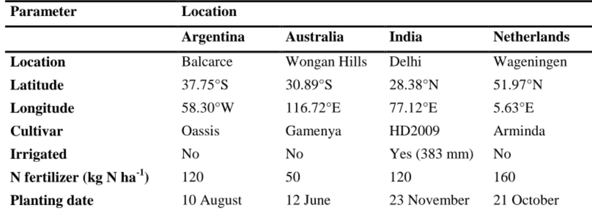
Table 1: Locations simulated in AgMIP Wheat Pilot (for more details see Martre et al., 2015) 203
Parameter Location
Argentina Australia India Netherlands
Location Balcarce Wongan Hills Delhi Wageningen
Latitude 37.75°S 30.89°S 28.38°N 51.97°N
Longitude 58.30°W 116.72°E 77.12°E 5.63°E
Cultivar Oassis Gamenya HD2009 Arminda
Irrigated No No Yes (383 mm) No
4 5 6 7 8 9 10 11 12 13 14 15 16 17 18 19 20 21 22 23 24 25 26 27 28 29 30 31 32 33 34 35 36 37 38 39 40 41 42 43 44 45 46 47 48 49 50 51 52 53 54 55 56 57 58
Anthesis date 23 November 1 October 18 February 20 June Harvest date 28 December 16 November 3 April 1 August
Year of experiment 1992 1984 1984-1985 1982-1983
204
Additional observations of yields in these regions potentially provide a target for accurate
205
interannual variability that the models are challenged to match. We therefore examined
1981-206
2010 national level yield data from the UN Food and Agricultural Organization
207
(http://faostat.fao.org/), overlapping district-level yields (in Australia; India: Ministry of
208
Agriculture, Government of India; and the Netherlands: Central Bureau of Statistics, the Hague,
209
STATLINE), and nearby variety trials (in Argentina: RET, www.inase.gov.ar; and the
210
Netherlands: Central Bureau of Statistics, the Hague, STATLINE) as a point of comparison
211
against simulated yields. It is not expected that these four modeling locations are precise
212
representations of the surrounding region; each represents carefully-controlled field trials in one
213
location within countries characterized by substantial differences in soils, climates, cultivars, and
214 management practices. 215 216 2.1.2 Wheat Models 217
Table 2 lists the 27 wheat models that simulated each of the four sites. Details of the processes
218
and parameter settings that distinguish each of these models are provided in the supplementary
219
material (particularly Table S2) of Asseng et al. (2013). The AgMIP Wheat Pilot’s first phase
220
agreed on a policy of model anonymity in the presentation of results, so for the purpose of this
221
study the models will be referred to only by a number assigned at random. This allowed us to
222
still determine the range of responses across these models’ native configurations and elucidate
223
how the selection of a crop model contributes to uncertainty in interannual yield simulations and
4 5 6 7 8 9 10 11 12 13 14 15 16 17 18 19 20 21 22 23 24 25 26 27 28 29 30 31 32 33 34 35 36 37 38 39 40 41 42 43 44 45 46 47 48 49 50 51 52 53 54 55 56 57 58
related decisions. The specific mechanisms for each model’s response are being considered in
225
ongoing analyses and future intercomparison design.
226 227
2.1.3 Types of simulation exercises
228
Wheat Pilot protocols were designed to investigate whether limitations in data (which hamper
229
the calibration of crop models in many locations) substantially affect the accuracy of yield
230
simulation and/or alter the simulated sensitivity to climate variability and climate changes.
231
Participants were therefore instructed to perform simulations in two steps:
232
1) Low-information simulations: Weather data, planting, crop emergence, flowering, and
233
physiological maturity dates, field management information, and soil characteristics and
234
initial conditions were provided but no information was provided on end-of-season yields
235
or in-season crop growth and soil water and nitrogen (N) dynamics. This subset of field
236
experiment data was referred to as “blind test” simulations by Asseng et al. (2013), and
237
represent the types of data that may be accessible for a large number of locations.
238
2) High-information simulations: In addition to the above data modelers were also provided
239
with in-season growth dynamics from the same years’ field trial, including, leaf area
240
index (all sites but AU), total above ground biomass and N, root biomass (at IN only),
241
cumulative evapotranspiration (at AU and IN only), plant available soil water and soil
242
inorganic N contents within the season (at AU and NL only), and end-of-season grain
243
yield and protein concentration, and grain density measurements. Plant components
244
(green leaves, dead leaves, stem, and chaff) biomass and N contents were also available
245
at NL. This full set of experimental data was referred to as “full calibration” simulations
4 5 6 7 8 9 10 11 12 13 14 15 16 17 18 19 20 21 22 23 24 25 26 27 28 29 30 31 32 33 34 35 36 37 38 39 40 41 42 43 44 45 46 47 48 49 50 51 52 53 54 55 56 57 58
by Asseng et al. (2013) and is equivalent to the more rare gold or platinum standards set
247
by Kersebaum et al. (2015) and Boote et al. (2015).
248
Analysis by Asseng et al. (2013) revealed a considerable reduction of biases between field
249
observations and yields using the high-information simulations, but noted that both the low- and
250
high-information simulations showed a similar response to changes in mean temperature and
251
CO2 concentrations.
252 253
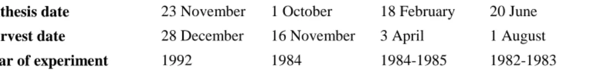
Table 2: Crop models included in AgMIP Wheat Pilot (in alphabetical order; for more information and details on 254
the processes modeled in each model see supplementary materials of Asseng et al., 2013) 255
Model Version Model description and
applications
Web address APES-ACE* V. 0.9.0.0 (Donatelli et al., 2010; Ewert et
al., 2011a)
http://www.apesimulator.it/default.aspx APSIM-Nwheats V.1.55 (Asseng et al., 2004; Asseng et
al., 1998; Keating et al., 2003)
http://www.apsim.info APSIM-wheat V.7.3 (Keating et al., 2003) http://www.apsim.info/Wiki/
AquaCrop* V.3.1+ (Steduto et al., 2009) http://www.fao.org/nr/water/aquacrop.ht ml
CropSyst V.3.04.08 (Stockle et al., 2003) http://www.bsyse.wsu.edu/CS_Suite/Cr opSyst/index.html
DSSAT-CERES-Wheat
V.4.0.1.0 (Hoogenboom and White 2003; Jones et al., 2003), (Ritchie et al., 1985)
http://www.icasa.net/dssat/
DSSAT-CROPSIM-Wheat
(Hunt and Pararajasingham 1995; Jones et al., 2003)
http://www.icasa.net/dssat/
Ecosys (Grant et al., 2011) https://portal.ales.ualberta.ca/ecosys/ EPIC wheat (Kiniry et al., 1995; Williams et
al., 1989) http://epicapex.brc.tamus.edu/ Expert-N - CERES - wheat ExpertN 3.0.10 Ceres 2.0
(Biernath et al., 2011; Priesack et al., 2006; Ritchie et al., 1987; Stenger et al., 1999) http://www.helmholtz-muenchen.de/en/iboe/expertn/ Expert-N - GECROS - wheat ExpertN 3.0.10
(Biernath et al., 2011; Yin and van Laar 2005; Stenger et al., 1999) http://www.helmholtz-muenchen.de/en/iboe/expertn/ Expert-N - SPASS - wheat ExpertN 3.0.10
(Biernath et al., 2011; Priesack et al., 2006; Stenger et al., 1999; Wang and Engel 2000)
http://www.helmholtz-muenchen.de/en/iboe/expertn/ Expert-N - SUCROS – wheat ExpertN 3.0.10 Sucros2
(Biernath et al., 2011; Goudriaan and Van Laar 1994; Priesack et al., 2006; Stenger et al., 1999)
http://www.helmholtz-muenchen.de/en/iboe/expertn/ FASSET V.2.0 (Berntsen et al., 2003) (Olesen et
al., 2002)
4 5 6 7 8 9 10 11 12 13 14 15 16 17 18 19 20 21 22 23 24 25 26 27 28 29 30 31 32 33 34 35 36 37 38 39 40 41 42 43 44 45 46 47 48 49 50 51 52 53 54 55 56 57 58 2010) 01.leeds.ac.uk/research/icas/climate_cha nge/glam/download_glam.html HERMES V.4.26 (Kersebaum 1995; Kersebaum
2007; Kersebaum 2011; Kersebaum and Beblik 2001)
www.zalf.de/en/forschung/institute/lsa/f orschung/oekomod/hermes
InfoCrop V.1 (Aggarwal et al., 2006) http://www.iari.res.in LINTUL-4 v.1 (Shibu et al., 2010; Spitters and
Schapendonk 1990)
http://models.pps.wur.nl/models LPJmL* (Bondeau et al., 2007; Fader et
al., 2010; Waha et al., 2012)
http://www.pik-potsdam.de/research/projects/lpjweb MCWLA-Wheat* V2.0 (Tao et al., 2009a; Tao and Zhang
2010; Tao et al., 2009b; Tao and Zhang 2011)
---
MONICA V.1.0 (Nendel et al., 2011) http://monica.agrosystem-models.com O'Leary-model V.7 (Latta and O'Leary 2003; OLeary
and Connor 1996a; b; Oleary et al., 1985)
Primary documentation for V7 (V3 (O'Leary and Connor 1996a; b), with incremental documentation thereafter.
SALUS V.1.0 (Basso et al., 2010; Senthilkumar et al., 2009)
www.salusmodel.net Sirius2010 (Jamieson and Semenov 2000;
Jamieson et al., 1998; Lawless et al., 2005; Semenov and Shewry 2011)
http://www.rothamsted.ac.uk/mas-models/sirius.php
SiriusQuality V.2.0 (Ferrise et al., 2010; He et al., 2011; He et al., 2010; Martre et al., 2006)
http://www1.clermont.inra.fr/siriusqualit y
STICS V.1.1 (Brisson et al., 2003; Brisson et al., 1998)
http://www6.paca.inra.fr/stics_eng/ WOFOST* V.7.1 (van Diepen et al., 1989; Supit
and van Diepen, 1994; Boogard et al., 1998)
http://www.wofost.wur.nl
256 257
The 1981-2010 historical simulations that form the bulk of these analyses also served as the
258
historical basis for climate change simulations conducted by each wheat-modeling group. The
259
same model configurations were therefore forced by the same climate time series and baseline
260
carbon dioxide concentrations but with historical temperatures adjusted by -3˚C, +3˚C, +6˚C, and
261
+9˚C every day of the year. As initial soil conditions and crop management (including sowing
262
date and nitrogen fertilizer application) were kept constant over the 30-year period, these
263
simulations allow for a comparison between model responses to interannual climate variability
4 5 6 7 8 9 10 11 12 13 14 15 16 17 18 19 20 21 22 23 24 25 26 27 28 29 30 31 32 33 34 35 36 37 38 39 40 41 42 43 44 45 46 47 48 49 50 51 52 53 54 55 56 57 58
and to mean climate changes. The re-initialization of soil conditions each year reduces the
carry-265
over effects of multi-year droughts, which reduces overall interannual variability. This is
266
common in agricultural modeling applications (particularly those that examine future climate
267
change where the sequence of events is more difficult to project than mean conditions), but
268
sequential simulations are an important developmental priority for more accurate representation
269
of extreme events and soil degradation (Basso et al., 2016) and crop rotation effects (Kollas et
270 al., 2015). 271 272 2.2 Performance of Ensemble 273
Martre et al. (2014) compared grain yield, protein content concentration, and in-season and
end-274
of-season variables within the 27 wheat model simulations against observations at each of the
275
four pilot locations. Although some models had the closest match to specific observations,
276
across all observed variables the 27-model unweighted arithmetic ensemble mean performed
277
best, in line with earlier findings based on smaller model ensembles even when used to
278
reproduce interannual yield statistics (Palosuo et al., 2011; Rötter et al., 2012). Thus, while each
279
wheat model has its own biases and accuracies, the errors across models tended to compensate
280
and the resulting ensemble had additional value (see also Challinor et al., 2014b). The superior
281
performance of the ensemble also reflected that wheat models have evolved with enough
282
independence in approaches to achieve a random distribution of biases for most variables rather
283
than leading to the emergence of common biases.
284 285
In light of the superior performance of the 27-member ensemble mean in reproducing field
286
observations across the four sites (and the lack of long-term historical yield observations at each
4 5 6 7 8 9 10 11 12 13 14 15 16 17 18 19 20 21 22 23 24 25 26 27 28 29 30 31 32 33 34 35 36 37 38 39 40 41 42 43 44 45 46 47 48 49 50 51 52 53 54 55 56 57 58
location), for the purposes of this study we utilize the full, 27-model unweighted arithmetic mean
288
ensemble as the basis for comparison of each model’s climate response.
289 290 2.3 Methods of analysis 291 2.3.1. Agro-climatic correlations 292
As each of the simulations held management constant throughout the 1981-2010 simulation
293
period and soils were re-initialized each year (with the exception of LPJmL, which did not
294
reinitialize soil water), interannual yield variability is a result of model responses to climate
295
factors. Chief among these are precipitation, temperature, and solar radiation, which are likely to
296
affect crop growth on a number of time scales. Here we focus on the effects of variability in
297
mean values over the growing season, using Pearson’s correlations against grain yield to
298
determine key sensitivities within each crop model. Additional variance is likely explained by
299
climate variables at sub-seasonal time scales (particularly when extreme conditions align with
300
vulnerable phenological stages), which merits further examination in future studies. Correlation
301
was chosen as a simple illustration of association between climate and crop model response,
302
although aspects related to non-linearity and thresholds may not be captured. Future work may
303
also consider associative metrics such as the probability of detection for extreme events as a way
304
of isolating important properties of observations and models (Glotter et al., 2016).
305 306
As most studies will not have the luxury of running all 27 wheat models, we investigate the
307
expected benefit of adding each additional member to a multi-model subset to converge on
308
behaviors captured by the full 27-model ensemble. Without running the full analysis it is not
309
possible to know whether the models that are available are among the best or worst for a given
4 5 6 7 8 9 10 11 12 13 14 15 16 17 18 19 20 21 22 23 24 25 26 27 28 29 30 31 32 33 34 35 36 37 38 39 40 41 42 43 44 45 46 47 48 49 50 51 52 53 54 55 56 57 58
site’s climate variability response, so we utilize an 80%-exceedance threshold as a practical risk
311
in simulation design. Results therefore focus on the correlations that would be exceeded by 80%
312
of the possible combinations for any number of combined models.
313 314
2.3.2 Agro-climatic clustering
315
We employed the k-means clustering technique to form clusters of wheat models that are
316
characterized by similar correlations between yield and growing season temperature,
317
precipitation, and solar radiation (with equal weighting for all). K-means is an iterative process
318
by which models are regrouped until silhouette values (i.e., similarity between each model and
319
the other members of its cluster) are maximized. For each location we examined the results with
320
three, four, and five clusters and visually selected the number that best captured cohesive
321
groupings in the climate-sensitivity space (this resulted in three clusters in both Argentina and
322
India and four clusters in both Australia and the Netherlands). Fewer clusters than this grouped
323
models with substantially different yield sensitivities to climate variability in the same cluster,
324
while more clusters tended to unnecessarily divide similarly-responsive models. As each model
325
belongs to a specific cluster at each location, we utilize the frequency that two models appear in
326
the same clusters across the four sites as a metric of model similarity.
327 328
3. Results and discussion
329
3.1 Baseline interannual variability
330
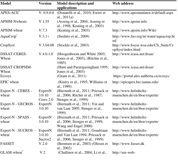
Figure 1 presents the 1981-2010 yields for the four Wheat Pilot locations from 27 wheat models,
331
the full model ensemble, and national and regional yields. These high-information simulation
332
results indicate uncertainty across the model ensemble, although common differences in mean
4 5 6 7 8 9 10 11 12 13 14 15 16 17 18 19 20 21 22 23 24 25 26 27 28 29 30 31 32 33 34 35 36 37 38 39 40 41 42 43 44 45 46 47 48 49 50 51 52 53 54 55 56 57 58
yield across the four locations are clear (as discussed by Asseng et al., 2013, and Martre et al.,
334
2015). Simulations exceed national and regional yields in each location, as wheat models often
335
do not include the effects of pests, diseases, poor crop management due to labor or equipment
336
shortages, waterlogging, and other factors that are common on farms outside of experimental
337
plots. Model results are therefore more representative of yield potential (Evans and Fischer,
338
1999) than the more complex conditions of a typical farmer’s field. The other source of
339
variation in the gray lines within Figure 1 comes from the less explored interannual variability of
340
simulated yields, which is the focus of analyses below. Interannual variability is reduced in the
341
model ensemble, as would be expected from averaging, although noteworthy variations suggest
342
that there are common behaviors across the crop model responses. Simulated yields (which
343
examine a single field) are characterized by greater interannual variance compared to the
344
national and regional level observations, likely because heterogeneities in soils, climate,
345
cultivars, and management reduces extreme year anomalies when aggregated to scales that may
346
exceed those of a given extreme event (Ewert et al., 2011b). Only variety trials (in Argentina
347
and the Netherlands) contain mean and variance of yields that are similar to the simulations,
348
although differences in management and the varieties cultivated also reduce the utility of these
349
records as a basis for truth in the comparison of models.
350 351
Discrepancies between various observational sources and the experimental field simulated by the
352
wheat models are large enough to caution against an expectation that the models would
353
reproduce national, regional, or trial-based observational records over the historical period.
354
These discrepancies are often due to the set up of the simulations from the single field
355
experiment not representing the diversity of soils, management and cultivars which affected the
4 5 6 7 8 9 10 11 12 13 14 15 16 17 18 19 20 21 22 23 24 25 26 27 28 29 30 31 32 33 34 35 36 37 38 39 40 41 42 43 44 45 46 47 48 49 50 51 52 53 54 55 56 57 58
regional and national yield data (but are not documented). Also, yield variability is often driven
357
by factors other than weather (Ray et al. 2015) and models that are driven by variations in
358
weather only are bound to not reproduce observational records. As noted above, we therefore
359
turn to the High-information ensemble average (dark line in Figure 1) as the standard for the
360
individual crop models given its superior performance in producing the full range of field
361
observations (Martre et al., 2015). The ensemble also reduces interannual variability through the
362
averaging of multiple models’ potentially uncorrelated anomalies.
363
364
3.2 Effect of calibration on climate sensitivity
365
The Wheat Pilot’s protocol for Low-information and High-information experiments provides a
366
useful examination of the ways in which model calibration has the potential to affect the
367
resulting response to climate variability. Figure 2 illustrates this sensitivity to calibration
368
information via the correlation of each individual model’s low-information results with the full
369
ensemble of Low-information simulations (LL), the correlation of each model’s Low-
370
information result with the full ensemble of High-information simulations (LH), and the
371
correlation of each model’s High-information results with the full ensemble of High-information
372
simulations (HH).
373 374
Correlations do not change dramatically between the Low- and High-information simulations for
375
the vast majority of wheat models at each of the four locations. The exceptions feature both
376
substantial improvements (e.g., Model #25 in Argentina) and declines (e.g., Model #10 in
377
Australia) in correlations as additional information is provided. In these cases calibration to
378
cultivars, soil conditions, or other internal parameters may have improved the experimental
4 5 6 7 8 9 10 11 12 13 14 15 16 17 18 19 20 21 22 23 24 25 26 27 28 29 30 31 32 33 34 35 36 37 38 39 40 41 42 43 44 45 46 47 48 49 50 51 52 53 54 55 56 57 58
year’s results but also affected climate sensitivity via shifts in the resilience to heat, water, and/or
380
frost stresses. Effects of calibration strategy on simulations of climate change impact were also
381
examined by Challinor et al. (2014b) and for simulations of crops across Europe (Angulo et al.,
382
2013). The relative lack of different sensitivities between the Low- and High-information
383
simulations could also be explained by the fact that each was simulated by the same model
384
experts for a given model, and that additional data provided for the High-information
385 386 387
4 5 6 7 8 9 10 11 12 13 14 15 16 17 18 19 20 21 22 23 24 25 26 27 28 29 30 31 32 33 34 35 36 37 38 39 40 41 42 43 44 45 46 47 48 49 50 51 52 53 54 55 56 57 58 388
Figure 1: Historical period grain yields for a) Argentina, b) Australia, c) India, and d) The Netherlands, including 389
the individual crop models at single simulation locations (gray lines), mutli-model ensemble mean (black solid line), 390
and observations from national, regional, and local field trial data. Linear trends were removed from observational 391
data at all but the Argentinian site (which had no significant trend). Modeled yields are the result of the high-392
information calibration simulations. 393
4 5 6 7 8 9 10 11 12 13 14 15 16 17 18 19 20 21 22 23 24 25 26 27 28 29 30 31 32 33 34 35 36 37 38 39 40 41 42 43 44 45 46 47 48 49 50 51 52 53 54 55 56 57 58
simulations were mostly limited to details on the crop itself. Additional information about the
395
soil environment, in particular, would have potentially altered the sensitivity to interannual
396
rainfall anomalies.
397 398
A comparison between the LL and HH correlations indicates that most models have the same
399
relationship with the full ensemble regardless of the level of calibration information. Where LH
400
and HH correlations are similar for a given model there is little benefit from additional
401
calibration in terms of interannual climate response, as the Low-information results perform just
402
as well as the High-information results against the High-information ensemble standard. HH
403
correlations are at least higher than LL correlations in the majority of cases, suggesting that
404
additional calibration information does tighten the spread of models around the ensemble mean
405
and thus improve the performance of several models. This benefit is blurred by the likelihood
406
that the fully-calibrated set of models would be expected to have closer agreement among
407
members; however, it is important to note that calibration data at each site were only provided
408
for a single year, making it impossible to directly calibrate the interannual variability examined
409
here. This is a typical limitation for crop model simulations, as there are few long-term field
410
trials that would allow full calibration of interannual variability. Also calibration in many cases
411
focuses on minimizing error between modelled and observed results for the calibration dataset,
412
which may have little influence on model responses to variation in environmental conditions that
413
may be controlled by model structure and parameters other than those in focus for the
414
calibration. The remainder of this study will focus on the High-information simulation sets, as
415
these are likely to be of highest fidelity. Agro-climatological mechanisms at the root of these
416
correlations are explored in Section 3.4 below.
4 5 6 7 8 9 10 11 12 13 14 15 16 17 18 19 20 21 22 23 24 25 26 27 28 29 30 31 32 33 34 35 36 37 38 39 40 41 42 43 44 45 46 47 48 49 50 51 52 53 54 55 56 57 58 419
Figure 2: Single model run correlations against ensemble mean during 1981-2010 for (a) Argentina; (b) Australia; 420
(c) India; and (d) The Netherlands. The correlation between the information model runs and the Low-421
information ensemble mean (LL) is displayed in light gray, the correlation between the Low-Information model runs 422
and the information ensemble mean (LH) is displayed in dark gray, and the correlation between the High-423
information model runs and the High-information ensemble mean (HH) is displayed in black. 424
4 5 6 7 8 9 10 11 12 13 14 15 16 17 18 19 20 21 22 23 24 25 26 27 28 29 30 31 32 33 34 35 36 37 38 39 40 41 42 43 44 45 46 47 48 49 50 51 52 53 54 55 56 57 58 425
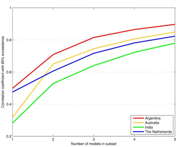
3.3 Benefit of multi-model ensemble
426
The 27-model community approach of the AgMIP Wheat Pilot is not possible in the vast
427
majority of crop model applications. Instead, what is needed is prior information that aids in the
428
construction of a practical subset of models with a high likelihood of representing the larger
429
ensemble. Beginning on the left-hand side of Figure 3 (representing the use of a randomly
430
selected single model), the plotted value represents the Pearson’s correlation (against the full
431
High-information ensemble) that would be exceeded by 80% of the individual models. This
432
value is highest for Argentina (where 80% of the models exceed r = 0.50) and lowest for India (r
433
= 0.28). Introducing a second model results in (27*26)/2=351 possible combinations, but 80%
434
of them have a correlation of at least r = 0.71 in Argentina and r = 0.53 in India. Across the four
435
sites, the benefit of adding a second model to a climate variability analysis is therefore an
436
increase of +0.23 in its likely correlation with the full ensemble, with gains highest in Australia
437
(+0.33) and lowest in the Netherlands (+0.13). Adding a third model also substantially increases
438
the 80%-likely correlation, although the average increase is reduced (+0.11). The additions of a
439
fourth and fifth model (increasing correlations by an average of 0.06 and 0.04, respectively) to
440
the subset are also beneficial and lead to very high correlations, but the increases begin to be
441
small in comparison to the effort likely required to calibrate an additional model (and collaborate
442
with an additional modeling group) for the effort.
443 444
Efforts to include a second and third model therefore provide substantial benefit to climate
445
variability simulations; however, investment in including additional models has a diminishing
446
return. These results suggest a benefit at smaller subsets to account for interannual climate
4 5 6 7 8 9 10 11 12 13 14 15 16 17 18 19 20 21 22 23 24 25 26 27 28 29 30 31 32 33 34 35 36 37 38 39 40 41 42 43 44 45 46 47 48 49 50 51 52 53 54 55 56 57 58
variability than the 5- to 10-member subsets that AgMIP crop model pilots identified as
448
beneficial by comparing multi-model convergence against the 13.5% error that is common in
449
field observations for wheat (Asseng et al., 2013) and maize (Bassu et al., 2014) or the 15%
450
observational error for rice (Li et al., 2014). The analyses were also conducted using a 70% and
451
90% threshold, with consistent patterns of benefit but the higher thresholds further emphasizing
452
the risks of the worst model being randomly selected.
453
454
Figure 3: Improvement in correlations with each additional model within a multi-model subset of the full ensemble. 455
For each number of models included in the subset N, the value shown represents Pearson’s correlation coefficient 456
between the subset’s mean yield and the full ensemble’s mean yield and that would be exceeded 80% of the time 457
given a random selection of N models from the full set of 27 wheat models. Simulations were performed at single 458
locations in each country (see Table 1) after calibration with High information, and all possible combinations of N 459
4 5 6 7 8 9 10 11 12 13 14 15 16 17 18 19 20 21 22 23 24 25 26 27 28 29 30 31 32 33 34 35 36 37 38 39 40 41 42 43 44 45 46 47 48 49 50 51 52 53 54 55 56 57 58 461 3.4. Agro-climatic Sensitivity 462
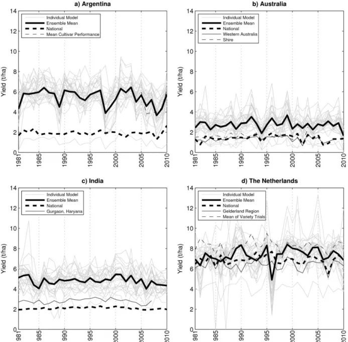
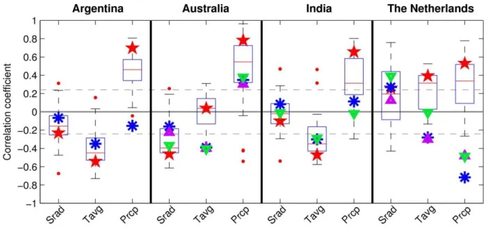
Correlations of the 1981-2010 modeled grain yields and observed grain yields with mean
463
growing season solar radiation, temperature, and precipitation are shown in Figure 4 across the
464
four locations. In Argentina simulated grain yields are positively correlated with wet seasons in
465
all but one model, with more than 75% of the models demonstrating significant correlations. A
466
strong sensitivity to rainfall anomalies is also seen in the cultivar trials; however, national grain
467
yields are not significantly correlated with the precipitation at Balcarce, Argentina, as the wheat
468
area covers a much larger region. The simulations and cultivar trials agree that lower
469
temperatures significantly favor grain yields, with even the national grain yields following suit as
470
warm and cooler seasons tend to spread more widely than the precipitation anomalies. At all
471
sites, for both temperature and precipitation, the magnitude of the ensemble average’s correlation
472
is substantially higher than that of the median model; indicating that precipitation and
473
temperature sensitivities are a unifying factor describing grain yield across the model members.
474
Solar radiation variability is not significantly correlated for the bulk of models.
475 476
The Australian location is characterized by an even stronger sensitivity to rainfall. This site is
477
also significantly sensitive to solar radiation anomalies, with negative correlations suggesting
478
interdependence as cloudier seasons correspond with wetter conditions. National and regional
479
yields are less responsive to precipitation anomalies and are governed more by temperature, as
480
temperature anomalies may be widespread while droughts in the east are often offset by wetter
481
conditions in the west.
482 483
4 5 6 7 8 9 10 11 12 13 14 15 16 17 18 19 20 21 22 23 24 25 26 27 28 29 30 31 32 33 34 35 36 37 38 39 40 41 42 43 44 45 46 47 48 49 50 51 52 53 54 55 56 57 58
Simulated yields at the Indian site are significantly correlated with precipitation despite irrigation
484
applications totaling 383 mm over the growing season using fixed application dates (as applied
485
in the field experiment). While an irrigation amount of 383 mm was sufficient for the 1984-1985
486
field trial, in other years the amount and timing of these applications may not have been adequate
487
to prevent water stresses from influencing crop growth and final yields. It is also possible that
488
precipitation anomalies are correlated with particular temperature and solar radiation regimes
489 490
491
Figure 4: Box-and-whiskers plots of Pearson’s correlation coefficients between the 27 wheat models’ 1981-2010 492
simulated grain yields at single locations in each country and corresponding growing season mean solar radiation 493
(Srad), average temperature (Tavg) and precipitation (Prcp). The median of the model simulations is marked by the 494
red line, the box contains the middle two quartiles (from 25% to 75%), and the whiskers extend to the most extreme 495
data points of the simulations that are not considered outliers (displayed as red dots). The correlation of the 496
ensemble performance (red star), national observations (blue asterisk), regional observations (magenta triangles; 497
where available), and the mean of other field trial results or local observations (green triangles) over the years data 498
were available are also presented (as in Figure 1). Dashed lines indicate thresholds for correlations that are 499
significant at the 90th percentile (t-test). 500
4 5 6 7 8 9 10 11 12 13 14 15 16 17 18 19 20 21 22 23 24 25 26 27 28 29 30 31 32 33 34 35 36 37 38 39 40 41 42 43 44 45 46 47 48 49 50 51 52 53 54 55 56 57 58
that are favorable for irrigated wheat growth. Cool seasons here are favorable for wheat
501
production, and solar radiation correlations are not significant. National level correlations with
502
the Delhi weather series are understandably weaker for all variables, as heterogeneous climate
503
across India’s wheat-growing regions reduces the prominence of anomalies and results in
504
insignificant correlations in all but average temperature.
505 506
Wheat at the Netherlands site follows a different agro-climatic pattern from that at the other three
507
sites. Warm seasons are positively correlated with yields in the bulk of models, suggesting a
508
growing degree day limitation. Simulations and observations also suggest a radiation limitation
509
at this high latitude, with sunnier seasons (and the associated temperature and rainfall patterns)
510
favoring higher yields. The field site is notably different from the regional and national level
511
observations in that the aggregated observations are either not correlated with temperature or
512
suggest that yields favor cooler temperatures. The models also indicate stronger yields in wet
513
years, while observations indicate better production during drier seasons. This likely comes
514
from the fact that local and regional management of shallow groundwater tables in this region
515
helps control against water stress but this management is not considered in the models at the test
516
site. Contrary to the models’ perception of drought, elevated regional yields are recorded in dry
517
seasons as higher solar radiation and groundwater provisions increase yield potential (Asseng et
518
al., 2000).
519 520
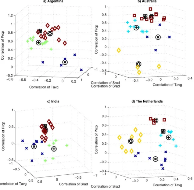
3.5. Clusters of agro-climatic response
521
Figure 5 shows each of the 27 wheat models as plotted on a three-dimensional space of
522
temperature, precipitation, and solar radiation correlations with that model’s grain yield. Models
4 5 6 7 8 9 10 11 12 13 14 15 16 17 18 19 20 21 22 23 24 25 26 27 28 29 30 31 32 33 34 35 36 37 38 39 40 41 42 43 44 45 46 47 48 49 50 51 52 53 54 55 56 57 58
falling in the same agro-climatic cluster are represented with a common symbol and color. The
524
full ensemble average and cluster averages do not fall as an average of the individual model
525
members’ correlations as the ensemble averaging reduces individual models’ yearly anomalies to
526
produce a unique time series. The results illustrate that the model spread is not randomly
527
distributed in the agro-climatic sensitivity space, but rather distinct families of responses are
528
evident. Several clusters also correspond much more closely with the full ensemble average
529
responses.
530 531
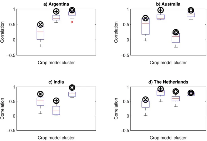
Figure 6 shows the spread of model correlations within each cluster as well as the cluster
532
ensemble correlations against the full 27-model ensemble’s interannual yield variability. One or
533
two clusters at each location demonstrate substantially better coherence to the ensemble average
534
than the others. Even within a given cluster there are substantial differences in correlation
535
between individual models and the ensemble average; particularly among clusters that are
536
furthest from the ensemble average sensitivities (e.g., the “x” cluster in Argentina or the diamond
537
cluster in Australia). The ensemble average for each cluster is also a marked improvement on
538
the median model within that cluster, although occasionally there is one model that outperforms
539
even the cluster mean.
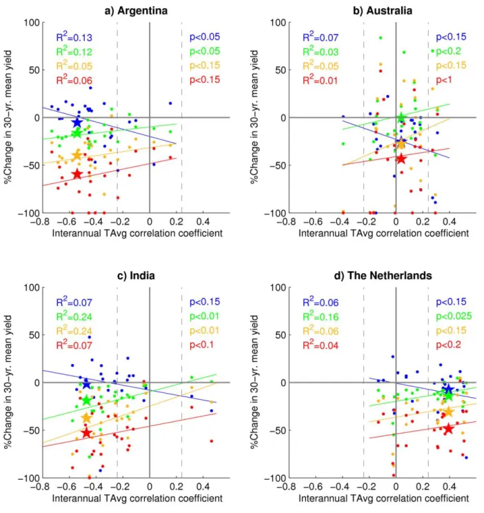
540 541 542
4 5 6 7 8 9 10 11 12 13 14 15 16 17 18 19 20 21 22 23 24 25 26 27 28 29 30 31 32 33 34 35 36 37 38 39 40 41 42 43 44 45 46 47 48 49 50 51 52 53 54 55 56 57 58 543
Figure 5: Clusters of the 27 wheat model simulations (cluster membership denoted by shape of symbols), the 544
ensemble average, and observational data according to their grain yield correlation coefficients versus mean growing 545
season solar radiation (Srad), average temperature (Tavg), and precipitation (Prcp) from 1981-2010 for single 546
locations in (a) Argentina; (b) Australia; (c) India; and (d) The Netherlands. The correlation coefficients of the 547
ensemble yield performance (boxed star) and the centroids of the clusters (corresponding symbols with circles) are 548
also presented. Note that the perspective is rotated and axes limits adjusted in each panel in order to best visualize 549
the differences in the model clusters. 550
551 552
4 5 6 7 8 9 10 11 12 13 14 15 16 17 18 19 20 21 22 23 24 25 26 27 28 29 30 31 32 33 34 35 36 37 38 39 40 41 42 43 44 45 46 47 48 49 50 51 52 53 54 55 56 57 58
Despite the fact that many of these wheat models have common heritage in pioneering crop
553
modeling groups and approaches developed in the last 30 years, only two pairs of models (#1/#5
554
and #20/#22 from Figure 2; making <0.3% of possible combinations and thus potentially just a
555
coincidence) fall in the same agro-climatic cluster at all four Pilot locations. 7% of model pairs
556
fall in the same cluster at three of the four sites, while 24% of model pairs are never in the same
557
cluster. The remaining 69% of model pairs share one or two clusters, which would be expected
558
for independent models. No individual model stands out as being particularly divergent from the
559
others, as each model has at least three other models that never appear in the same cluster, and at
560
least four models that fall in the same cluster for two or more sites. Only one model falls into the
561
highest-correlating cluster at all four locations, and likewise only a single model always falls into
562
the lowest-correlating cluster. In total 15 different models are included in the lowest-correlating
563
cluster for at least one site, and 21 different models are part of the highest-correlating cluster at
564
least once. This independence likely contributes to the strength of the full ensemble, as more
565
independent models are less likely to share common response biases. Model similarities and
566
differences from site to site also cautions against assuming that performance of a given model at
567
a limited number of sites is indicative of its likely performance at a new site. The high
568
sensitivity of the models’ response to climate variability demonstrates high sensitivity to
569
location, representing different growing environments. Results suggest that there is little basis
570
on which to categorize groups of models based upon expected commonalities in climate
571
variability response, as these responses show high sensitivity to location rather than models
572
imposing the same response to all sites.
573 574
We created subsets of models with the rule that only one model could be drawn from each
4 5 6 7 8 9 10 11 12 13 14 15 16 17 18 19 20 21 22 23 24 25 26 27 28 29 30 31 32 33 34 35 36 37 38 39 40 41 42 43 44 45 46 47 48 49 50 51 52 53 54 55 56 57 58
cluster to test the hypothesis that diverse model combinations would more efficiently capture
576
responses of the full ensemble than would a random combination of wheat models. However,
577
performance of these subsets was not significantly different from the random subsets tested in
578
Section 3.3 above. Selecting more diverse models via cluster analysis is therefore not an
579 580
581
Figure 6: Correlations between simulated grain yield by the wheat models against the 27-member ensemble average 582
series of interannual grain yields for single locations in (a) Argentina; (b) Australia; (c) India; and (d) the 583
Netherlands. The correlations of the cluster ensembles are shown in the dark black symbol above the box-and-584
whiskers distribution of individual models within that cluster (corresponding to the symbols from Figure 5). 585
586
effective strategy for creating multi-model subsets for new studies, although the construction of
587
subsets based upon model structure and parameter sets (rather than response characteristics)