Career Path Analysis of Professionals Selected by MIT Undergraduates by
Kyle Pina
Submitted to the
Department of Mechanical Engineering
in Partial Fulfillment of the Requirements for the Degree of Bachelor of Science in Mechanical Engineering
at the
Massachusetts Institute of Technology June 2018
C 2018 Kyle Pina. All rights reserved.
The author hereby grants to MIT permission to reproduce and to distribute publicly paper and electronic copies of this thesis document in whole or in part in any medium now known or
hereafter created.
Signature redacted
Signature of Author:
7
7
i 11Signature redacted
Department of Mechanical Engineering May 11, 2018 Certified by:
J
Warren Seering-MASS AHusETTS INSTIUTE OF TECHNOLOGY
SEP 13 2018
LIBRARIES
ARCHIVES
Weber/Shaughness Professor of Mechanical Engineering
Signature redacted
Thesis SupervisorRohit Karnik Associate Professor of Mechanical Engineering Undergraduate Officer Accepted by:
Career Path Analysis of Professionals Selected by MIT Undergraduates by
Kyle Pina
Submitted to the Department of Mechanical Engineering on May 11, 2018 in Partial Fulfillment of the
Requirements for the Degree of
Bachelor of Science in Mechanical Engineering
Abstract
For current MIT undergrads, life after graduation can seem daunting. With uncertainty about job duration, graduate school, and career paths in general, many undergraduates enter the real world unsure of what the future holds, or if what they have decided to do post-graduation is the "best" option. As such, MIT undergraduates in the Undergraduate Practice Opportunities Program (UPOP) were asked to interview professionals that they believed had jobs they would one day also like to have. This resulted in a large dataset of career paths for an extremely diverse group of individuals, all with their own unique stories and time-lines. This data was filtered, cleaned, and analyzed to gain insight into life after graduation. From the analyzed data it was found that the distributions of durations spent at graduate school, in companies, or in specific job titles were all not significantly different, and the average duration spent in each of these options was 2-6 years, with some noticeable outliers. Overall these analyses showed that there are many options for students in the first 10 years after completing their BS, and there is no clear "correct" option to choose from.
Thesis Supervisor: Warren Seering
Title: Weber/Shaughness Professor of Mechanical Engineering
Acknowledgments
The author would like to thank Professor Warren Seering, Jim Margarian, and the UPOP staff for their support during this research.
Table of Contents
A bstract ... 2
A cknow ledgm ents... 2
1. Introduction ... 4
2. Prelim inary W ork ... 5
2.1. D ata Collection... 5
2.2. Population Sum m ary Statistics... 6
2.3. D ata Filtering and Cleaning ... 8
3. Results of D ata A nalysis... 9
3.1. Com pany and Graduate School Duration A nalysis... 9
3.2. Post Bachelor of Science - Ten Year Analysis ... 15
3.3. Com pany and Job Changing A nalysis ... 20
4. Specific Case Studies... 29
4.1. M asters Students Period 1... 29
4.2. PhD Students Period 1... 33
4.3. N o Graduate School Period 1... 36
5. Conclusions ... 41
6. Appendices ... 43
6.1. 2017 Com pany D uration Kruskal-W allis Box Plot... 43
6.2. 2016 Com pany 1 D uration D istributions ... 44
6.3. 2016 Com pany 3 D uration D istributions ... 50
6.4. 2015 Com pany Duration D istributions... 53
6.5. 2015 Com pany 3 D uration D istributions ... 59
1. Introduction
MIT undergraduates currently face much uncertainty as they enter their senior years. As they begin to consider whether to go into industry, pursue graduate studies, or simply take time off, there are many questions that arise within the undergraduate community about what is
considered the "correct" career move. Currently there is no factual or data-based advice available to undergraduates regarding career paths, and they must rely on word of mouth advice from specific individuals who may or may not have similar career interests or goals. In order to
answer this question of what is the "correct" career move after finishing undergraduate studies at MIT, or dismiss it altogether, sophomore undergraduates from the years 2015, 2016, and 2017 participating in the Undergraduate Practice Opportunities Program (UPOP) were asked to interview professionals who had jobs and positions that they would one day also like to have. The UPOP program is a career development program available to sophomore undergraduates at MIT. The interviews were conducted during the UPOP students' respective summers and consisted of a standardized survey asking first general demographic information, and then specific career path information. The survey itself remained relatively the same in 2015 and 2016, and then changed dramatically in 2017. As such, the 2017 survey is used more heavily in this research as it reveals deeper insights into individual career paths.
From the collected data, preliminary analysis was done to characterize the interviewee population in terms of age and job title. Next, the data was filtered and cleaned so that only interviewees who had received a Bachelor of Science (BS) were considered to better match the MIT undergraduate population administering the survey. From there, duration distributions were analyzed for time spent in graduate school and time spent at companies for each career period given. Next, a ten-year, post BS analysis was conducted to gain better insight into the early years post undergrad. After this, the frequency of changing companies compared to changing jobs within the same company was studied. Finally, specific case studies were done to gain better career path insight into specific subpopulations, such as those who pursed a Master of Science (MS) or a Doctor of Philosophy (PhD) post BS, or those who never attended graduate school immediately after their BS.
2. Preliminary Work
2.1. Data Collection
Data for this study was collected by students in the UPOP program via surveys that were used as an interview template. UPOP students were given the freedom to choose who they interviewed, with the condition that the interviewee had a job or position that the UPOP student would one day also like to have. The same survey was used by every UPOP student to allow for standardized responses that would then allow for proper analysis.
For the years 2015 and 2016, the survey was essentially the same, and focused primarily on interviewees work experience. The survey began asking for the student's basic information such as name, major, and what they were pursuing over the given summer. The survey then asked about the interviewee, asking for current work and industry information, their relationship to the student, and what degrees they currently held. The rest of the survey focused on the
interviewee's career path, asking first about the interviewee's most recent company and what job title, or titles, they had at said company. The survey then worked backwards along the
interviewee's career path, asking for what companies they had previously worked for and what titles they had at each respective company, and for how long. Students were allowed to enter up to five job titles at each company and were allowed to enter three different companies in total. If the interviewee had worked at more than three companies or had more than five job titles at a
single company, this was recorded in additional questions asking how many more job titles the interviewee had at a specific company beyond the five titles that were entered, or how many more companies the interviewee had worked at beyond the three companies that were entered.
By the nature of these surveys, the 2015 and 2016 data were most useful for analyzing company duration, and the frequency of interviewee's changing companies compared to changing jobs within the same company.
The 2017 survey had a dramatic rework from the 2015 and 2016 surveys. Beginning with the same general questions as the 2015 and 2016 surveys regarding student and interviewee
information, the survey then asked students to work from the beginning of the interviewee's career path in sequential periods. In each period, the student defined the start and end year of the period, and then listed any relevant academic or industry roles. For academic roles, the students could enter a degree type, a degree field, and an academic institution or university. For the industry roles, the students could enter a company or organization name, a field or industry, and then up to six different job titles. Unfortunately, they could not specify a duration for each job title. A maximum of eight periods were allowed to be entered, however the most periods entered by students was six. At the end of the survey were open ended questions, which were intended to give qualitative information about the interviewee's career path. With much more information but less granularity in terms of duration of specific job titles within companies, the 2017 data was extremely useful for analyzing both company and graduate school durations, and specific case studies for subpopulations of the general survey population, such as for MS and PhD degree holders. The way the 2017 data was structured also allowed for a ten-year, post BS analysis to
gain insights into the early years after finishing undergraduate studies, which is of much interest to MIT undergraduates.
2.2. Population Summary Statistics
Before the data was filtered and cleaned, summary charts were made to gain a better understanding of the interviewee population. The first question of interest was the general ages of the interviewee population. Only the 2017 survey asked students to estimate the interviewee's age, so there is no age data from years 2015 or 2016. However, the general age trends most likely hold in previous years and can be used to generalize the entire interviewee population over the three years. Exact ages of interviewees were not asked for. Rather, students were asked to estimate their interviewees age simply based on looks. The summary of age information is shown in figure 1. For all figures presented the number of samples in each figure (n = #) and which data set the data in the figure is from (e.g. 2017) is given.
Interviewee Ages 100 - 97 n =264(2017)-90 - 85 80 70 -60 -50 -40 35 34 30 20 11 10 1 1 0
Figure 1: Survey interviewee age distribution. A little over one third of interviewees were in their 30s, and roughly 85% of interviewees were in their 30s or 20s. This chart shows MIT undergraduates general interest in younger professionals, most likely because they are more
From the compiled data over a third of the interviewees were in their 30s, and roughly 85% of interviewees were in their 30s or 20s. This shows general MIT undergraduate interest in young professionals, most likely because they are more relatable, and can provide more recent perspective on post BS career choices.
The next question of interest was regarding interviewee's current jobs. Many different job titles were recorded by the students, but all the entries could be grouped into four distinct
categories; managers and executives, engineers, university people, and other. These general categories were chosen because they were the categories of highest interest among the UPOP students administering the survey. The other category consisted of job titles such as lawyers, doctors, consultants, and venture capitalists. All three survey years asked for current job titles of the interviewees, so all three years of data are represented in the job title summary. The job title
distribution summary of the interviewee population is shown in figure 2.
300 250 200 150 100 50 0 .SV: ec; Oro K09 02,
Job Title Distribution
979 n = 803 (2017, 2016, 2015)
229
198
104
Figure 2: Survey interviewee job title distribution. 74 more managers and executives were interviewed than engineers. Overall 33% of the interviewees were managers or executives,
25% were engineers, 13% were university people, and 29% had some other job title such as consultant or venture capitalist.
e X e
0f
\e
Somewhat surprisingly, 74 more managers and executives were interviewed than
engineers. For the overall interviewee population, 33% were managers or executives, 25% were engineers, 13% were university people, and 29% had some other job title. The higher proportion of managers and executives being interviewed could indicate general interest among MIT undergrads in one day pursuing managerial roles.
2.3. Data Filtering and Cleaning
After acquiring summary statistics for the interviewee population, the data was then filtered and cleaned. Because the 2017 survey was changed dramatically from the 2015 and 2016
surveys, both groups of surveys had to be filtered and cleaned separately.
For the 2017 survey, data entries were first filtered to limit the sample to only those who had received a BS in the first given period, or period 0. After this, remaining entries were filtered to ensure a graduation year was given. From here, remaining entries were filtered to ensure that if the interviewee had received a BS in period 0, and a graduation year was given, that data for the next period, period 1, was also given. Successive periods were then filtered, as entries stopped after a variety of given periods. What resulted was matrices for each period, with each row describing a specific entry. The first period totaled 153 entries, and by the sixth period only 16 entries remained. In order to keep track of specific entries across many periods of filtering, a unique entry ID was assigned to each entry and filtered in the same sequence as the data itself. With the unique entry ID in place, the matrices for each period could be merged together to create one large table where every row refers to a specific entry, and every column refers to a specific variable, for instance, "Period 4 Job 2". Upon visual inspection of this table, some ambiguous and erroneous entries were found. For example, while it is possible interviewees could have been both working and doing graduate studies, some entries carried the graduate school information in, say, period 1, across all periods thereafter. Rather than assume when each of these interviewee's graduate studies ended, all entries that contained both graduate school information and work information in the same period were removed. However, some entries that listed both graduate school and work information were either clearly working or clearly in school. For instance, some entries that listed graduate school information also listed the place of graduate study and research as the interviewee's work information for that period. Entries such as this were able to be manually corrected. Overall from 325 initial entries, the 2017 data set was filtered and cleaned down to 119 entries.
For the 2015 and 2016 surveys, the initial entries were first filtered by degrees the interviewees held. Since these surveys asked students to list all the degrees the interviewee possessed at the beginning of the survey rather than list them out as they were acquired as in the 2017 survey, it was assumed that interviewees who held masters and PhD degrees also held BS degrees. From here, remaining entries were filtered to ensure a graduation year was given. Overall from 319 initial entries for 2015 and 162 entries for 2016, the 2015 data set was filtered down to 174 entries and 2016 was filtered down to 76 entries.
3. Results of Data Analysis
3.1. Company and Graduate School Duration Analysis
The first study conducted on the 2017 data set involved comparing the durations of work at companies and the durations at graduate schools for each period. The 2017 survey was formatted so students would end a given period when the interviewee switched companies or finished a graduate degree. As such the following study aims to compare the duration distributions of time spent with companies with the duration distribution of time spent working on graduate degrees. The company duration distribution for period 1 is shown below in figure 3. For this figure, and all future duration distributions, "0 years" means the interviewee was with the given company or graduate school for less than 1 year.
15 10 I 0 0 5 0 0
Period 1 - Company Durations
I I n = 55 (2017)
1
--HTiI
5 IiI 10 15 Period Duration 20 (Years) 30 25Figure 3: Period 1 company duration distribution from the 2017
is skewed to the right and has a mean of 4.6 years, and median deviation of 6.2 years.
data set. The distribution 2 years, and a standard
The company duration distribution for period 1 is significantly skewed to the right with a mean of 4.6 years, a median of 2 years, and a standard deviation for 4.6 years. While the clear majority stayed with their first company for less than 5 years, there are noticeable outliers of 15 or more years, indicating some interviewees did find long term security and comfort in their first
9
-job after receiving their BS. The graduate school duration distribution for period 1 is shown below in figure 4. 18 16 -14 12 10 -0 U 8 6 4 2 0
Period 1 - Graduate School Durations
I I I I I I
0 1 2 3 4 5 6 7
Period Duration (Years)
Figure 4: Period 1 graduate school duration distribution from the 2017 data set. The distribution is slightly skewed to the right and has a mean of 3 years, and median 2 years, and a
standard deviation of 2 years.
The graduate school duration distribution for period 1 is slightly skewed to the right, but much less skewed to the right than the company duration distribution for period 1. Overall the distribution has a mean of 3 years, a median of 2 years, and a standard deviation of 2 years. These statistics are fairly similar to the company duration distribution, and the differences that are present are due to the large outliers in the company duration distribution for period 1. To compare the distributions, a Mann-Whitney U Test was used. The Mann-Whitney U Test is a statistical test very similar to the student t-test in that they are both used to compare independent groups, however the Mann-Whitney Test does not require the assumption of a normal population distribution. Since the population distribution in this case is unknown, we will assume it is not normal, warranting the use of the Mann-Whitney Test. In order for the Mann-Whitney test to be valid, four assumptions must be met: the dependent variable should be ordinal or continuous; the independent variable should consist of two categorical, independent groups; observations should be independent; and the distributions of the independent variables should have similar shape. In
this case; the dependent variable is continuous since it is measured in number of years, the two independent variables are company and graduate school, observations are assumed independent since every student interviewed a different professional, and both distributions have similar shape in that they are both skewed to the right. With all assumptions met, the Mann-Whitney test can be used. The null hypothesis of the Mann-Whitney test is that the distributions are the same. If a p-value of 0.05 or less is found from the test, we reject the null hypothesis and can say with 95% confidence that the distributions are different. The results of the test on period 1 company and graduated school durations yielded a p-value of 0.87. Since the p-value is greater than 0.05, we accept the null hypothesis, meaning the distributions are effectively the same. This implies that there is no significant difference in period 1 durations between the graduate school and working subpopulations.
This same analysis was then done on period 2 data. The company period 2 is shown below in figure 5.
I
II
5
duration distribution for
Period 2 - Company Durations
I
I
10 Period 15 20 Duration (Years) 25 30Figure 5: Period 2 company duration distribution from the 2017 data set. The distribution is skewed to the right and has a mean of 4 years, and median 3 years, and a standard
deviation of 4.5 years.
Similar to the period 1 company duration distribution, the period 2 company duration distribution is significantly skewed to the right, with a mean of 4 years, a median of 3 years, and
4A 0 C. 12 -10 -8 6 4 2 0 0
a standard deviation of 4.5 years. Also, like the period 1 company duration distribution, the majority of interviewees in period 2 stayed with their second company for less than 5 years, but there are again some interviewees who found long term comfort in their second company. The graduate school duration distribution for period 2 is shown below in figure 6.
9 8 7 6 5 0 04 3 2 1 0
Period 2 - Graduate School Durations
1 2 3 4 5 6
Period Duration (Years)
Figure 6: Period 2 graduate school duration distribution from the 2017 data set. The
distribution is roughly normal and has a mean of 3.3 years, and median 3 years, and a standard deviation of 1.5 years.
The period 2 graduation school duration distribution is roughly normal with a mean of 3.3 years, a median of 3 years, and a standard deviation of 1.5 years. These statistics are very similar to the period 2 company duration distribution, with differences once again due to the significant outliers present in the company duration distribution. Although the distributions no longer have similar shape, breaking assumption four of the Mann-Whitney test, this assumption is only necessary when wanting to specifically compare medians of the distributions. With different shaped distributions, we are still able to compare the means of the distributions. Since we are only concerned with the distributions in general, and not specifically medians or means, the Mann-Whitney test is still valid. The results of the test on period 2 company and graduate school durations yielded a p-value of 0.41. Since the p-value is greater than 0.05, we accept the null hypothesis, meaning the distributions are effectively the same. This implies that there is no
significant difference in period 2 durations between the graduate school and working subpopulations, as was the case with period 1.
There were only 5 entries for graduate school durations in period 3, so beyond period 2, company and graduate school duration distributions were not able to be compared. However, company duration distributions up to period 5 contained enough data to be compared. As such, period 1 through 5 company duration distributions were compared using the Kruskal-Wallis H Test. This test is an extension of the Mann-Whitney U test, but for more than two categorical,
independent groups. The null hypothesis for the Kruskal-Wallis test is that all groups are from the same population. All of the same assumptions apply as before, but now the categorical groups are the different periods rather than company and graduate school. Period 3 through 5 company duration distributions are shown below in figures 7, 8, and 9.
0
Period 3 - Company Durations
5 10 15
Period Duration
20
(Years)
Figure 7: Period 3 company duration distribution from the 2017
is skewed to the right and has a mean of 5.6 years, and median deviation of 6.8 years.
25 30
data set. The distribution
3 years, and a standard 16 14 12 -10 -0 0 n = 59 (2017) i
L
I1
1
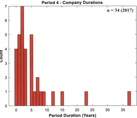
8 6 4 2 07 6 5 4 3 2 0 0 5 10 15 20 Period Duration 25 (Years) n = 34 (2017) 30 35
Figure 8: Period 4 company duration distribution from the 2017 data set.
is skewed to the right and has a mean of 5.3 years, and median 3 years, deviation of 7.4 years.
The distribution and a standard
Period 4 - Company Durations
I I I I I
0
0
I
I I
Period 5 - Company Durations 8 1 n 21 (2017) 7 6 5 -3 -- 2-0 3 --0 0 5 10 15 20
Period Duration (Years)
Figure 9: Period 5 company duration distribution from the 2017 data set. The distribution is skewed to the right and has a mean of 3.9 years, and median 2 years, and a standard
deviation of 5.3 years.
The p-value returned by the Kruskal-Wallis H Test was 0.39. Since this p-value is larger than 0.05, we accept the null hypothesis that all the groups are from the same population, meaning they are not significantly different from one another. This shows that as careers
progressed, interviewees tended to stay with companies for similar amounts of time each period. Overall this analysis shows that across periods for both company durations and graduate school durations, interviewees tended to stay in each period for the same amount of time. From the means and medians of the all the distributions, this amount of time is roughly 2-6 years.
3.2. Post Bachelor of Science - Ten Year Analysis
The second study conducted on the 2017 data involved a detailed analysis of the
interviewee's first ten years after finishing their undergraduate studies and acquiring their BS. Starting with the graduation years for each entry, the year being checked was incrementally compared to each successive period's given start and end year. For each increment of the year being checked, it was first determined which period the resulting year fell in, and then it was determined whether the interviewee was in work, in graduate school, or taking time off during
the specific period. As was mentioned previously in section 2.3, although it is possible the interviewee could have been both working and in graduate school, some students carried graduate school information entered in early periods across all periods thereafter. Because of this, all entries containing both graduate school and work information in the same period were removed, with a few exceptions that were also mentioned in section 2.3. The resulting ten-year analysis is shown below in figures 10 and 11. Figure 10 shows the number of entries for each year, and figure 11 shows percentage of entries for each year. Here, and for future similar figures, ni refers to the number of samples in year 1, and nio refers to the number of samples in year 10.
10 Year Post BS General Breakdown
4 5 6 7 Years From BS ni = 118 (2017) nio = 62 (2017) Gap Year Working In School 8 9 10
Figure 10: General ten-year post BS analysis for the 2017 data set by raw count for each
year. Year 1 begins with 118 entries, and by year 10 only 62 entries remain. 120 1 0 0 00 -80 60 40 -20 -0 1 2 3 1
..
.1
10 Year Post BS General Breakdown 100 90 -n= 118 (2017) 80 -nio =62 (2017) 70 -60 -Gap Year 50 - Working In School i 40 -a. 30 -20 -10 --0 1 2 3 4 5 6 7 8 9 10 Years From BS
Figure 11: Ten-year post BS analysis for the 2017 data set by percentage of entries for each year. The same number of entries are present in each year as shown in figure 10. Interesting trends can be seen upon visual inspection of these two figures. For the first 5 years after acquiring a BS, the proportion of interviewee's in graduate school or working is about the same in each year, around 50-55% for graduate school and around 40-45% for work with around 5-10% taking time off. Starting at year 6 and ending at year 10, the proportion of
interviewee's in work begins to increase while the proportion in graduate school decreases. By year 10, roughly 90% of interviewees are working while only 10% are in graduate school. It
should be noted that in these figures, it is possible for an interviewee to jump between bars each year. For example, and interviewee could work in their first year after receiving their BS and be in the red column for year 1, then in year 2 go back to school and be in the blue column for years 2 and 3, and then in year 4 return to work and be in the red column in year 4.
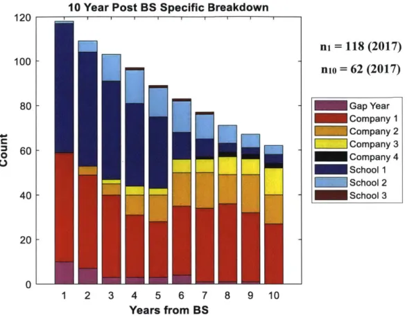
To go more in depth on this ten-year post BS analysis, the same charts were replicated, but this time keeping track of how many different graduate schools the interviewee attended and how many companies each interviewee worked for. These more detailed charts are shown below in figures 12 and 13. Figure 12 shows the number of entries for each year, and figure 13 shows percentage of entries for each year.
10 Year Post BS Specific Breakdown 120 I ni = 118 (2017) 100 - nio =62 (2017) 80 - Gap Year Company 1 Company 2 C -Company 3 60 Company 4 School 1 40I-USchool 2 40 School 3 20 0 1 2 3 4 5 6 7 8 9 10 Years from BS
Figure 12: Ten-year post BS analysis for the 2017 data set broken down by specific job
and school number. Each bar shows the raw number of entries for each year. The same number of entries are present as figures 10 and 11. The figure is essentially the same as figure 10, but each red and blue bar is broken into specific job and school numbers.
10 Year Post BS Specific Breakdown 100 r90 80 -70 -60 -50 -40 30 20 10 1 2 4 5 6 7 Years from BS
Figure 13: Ten-year post BS analysis for the 2017 data set broken down by specific job
and school number. Each bar shows the percentage of entries for each specific year. The same number of entries are present as figures 10 and 11. The figure is essentially the
same as figure 11, but each red and blue bar is broken into specific job and school numbers.
With this further breakdown of the previous figures, more insight can be gained into how many jobs interviewees had or how many different graduate schools interviewees attended in their first 10 years about receiving their BS. To begin, some interviewees were in their second
job as early as year 2, some were in their third job as early as year 3, and some were in their
fourth job as early as year 7. In terms of graduate school, one interviewee was already pursing their second degree beyond their BS in year 1, as they finished their first degree beyond their BS the same year they received their BS, a few of interviewees were pursuing their third degree beyond their BS by year 4, and some interviewees were pursuing their first degree beyond their BS 10 years after they received their BS.
Overall, these plots are very useful in seeing how specific proportions of the interviewee population change in the first ten years after acquiring a BS. The first ten years after the BS is of high interest to the students who administered the survey, and through this analysis these
students can see that there are many different options available to them the first ten years out of undergraduate studies. 8
L
IM 0 0 ni = 118 (2017) nio = 62 (2017) Gap Year Company 1 Company 2 LI Company 3 Company 4 School 1 School 2 School 3 9 10'7L
3.3. Company and Job Changing Analysis
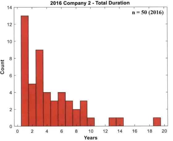
As was mentioned previously, the 2015 and 2016 data had more granularity than the 2017 data in terms of time spent with a specific job title vs time spent overall at a specific company. This extra granularity allows for comparison between the distributions of durations of job titles and the distributions of durations at companies. The distribution of total duration in company 2 for the 2016 data set is shown below in figure 14. It should be noted that company 2 here is in reference to the second most recent company the interviewee has worked for. Company 2 was specifically chosen because it had the highest number of samples of the three companies entered in the data set.
14 12 10 0 U 8 6 4 2 0
2016 Company 2 - Total Duration
0 2 4 6 8 10
Years
n = 50 (2016)
IF-FM
i '.12 14 16 18 20
Figure 14: Distribution of total company 2 durations for 2016 data. The distribution is
skewed to the right and has a mean of 4.5 years, a median of 3 years, and a standard deviation of 3.9 years.
This distribution is significantly skewed to the right with a mean of 4.5 years, a median on 3 years, and a standard deviation of 3.9 years. Overall the distribution shows that interviewees tend to stay at the same company for shorter periods of time rather than longer. This pattern holds for companies 1 and 3 as well. These duration distributions are in appendices 6.2 and 6.3
distribution company 2.
for company 2 can then be compared to the duration of specific job titles within The distribution of first job title durations is shown below in figure 15.
16 14 -12 -10 0 U 8 6 4 2 0
2016 Company 2 - Job Title I Duration
n = 49
(2016)
0 2 4 12 14 16 18 20
Figure 15: Distribution ofjob title 1 company 2 durations for 2016 data. The distribution
is skewed to the right and has a mean of 4 years, a median of 3 years, and a standard deviation of 3.9 years. These statistics match almost identically to the total company 2 duration distribution. Note that the number of samples here forjob title 1 is 1 less than the number of samples for the total company duration distribution. This was a result of
some students inaccurately entering job title duration information (e.g. accidently entering job title 1 information in job title 2). This error does not affect our analysis, are
we are only interested in job title durations, and not what order they occur in.
This distribution is also significantly skewed to the right with a mean of 4 years, a median of
3 years, and a standard deviation of 3.9 years. These statistics are nearly identical to the total
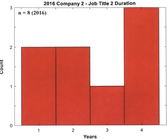
company distribution, and with a similar sample size, this indicates that the majority of the total company distribution is from the first job title for company 2. This is confirmed when looking at the distribution of the second and third job titles for company 2. These are shown in figures 16 and 17 respectively, below.
0
IFT]
' ,-6 8 10 Years I 1 03 2 .0 0 1 0
2016 Company 2 - Job Title 2 Duration
n =8 (2016)
I I I I______________ I I I II
1 2 3 4
Years
Figure 16: Distribution ofjob title 2 company 2 durations for 2016 data. With only a
sample size of 8, no summary statistics were taken for this distribution. This, along with figure 17 support the fact that the majority of total company 2 distribution is from the
0
0
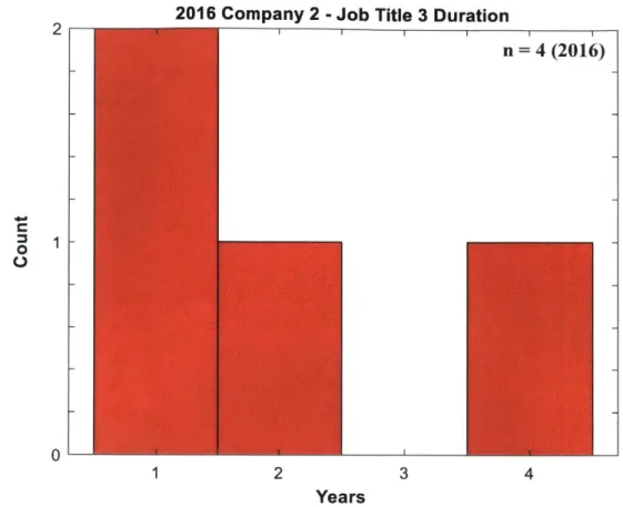
2016 Company 2 - Job Title 3 Duration
n I(2
n =4 (2016)
1 2 3 4
Years
Figure 17: Distribution ofjob title 3 company 2 durations for 2016 data. With only a sample size of 4, no summary statistics were taken for this distribution. This, along with
figure 16 support the fact that the majority of total company 2 distribution is from the first job title, whose distribution is shown in figure 15.
While no summary statistics were taken for the job title 2 and 3 distributions, the small sample sizes of both indicate that indeed the majority of the total company 2 duration
distribution is from the first job title. Another interesting observation is for both the second and third job title distributions, the longest duration for both is 4 years. This further supports the
observation from the total company 2 duration distribution that interviewees tended to stay with a specific company for shorter amounts of time rather than longer, since the maximum 4 years is located with the majority of the data and fits the skewed right trend. Overall this tends the show that there is no noticeable difference between duration with a specific job title and duration with a specific company, although this will be analyzed further later. Job title duration distributions for companies 1 and 3 are located in appendices 6.2 and 6.3 respectively.
This same analysis was then done on the 2015 data set, which showed similar results to the 2016 data set. The total duration distribution for company 2 in 2015 is shown below in figure 18. As was before, company 2 here refers to the second most recent company the interviewee has worked for. Like in the 2016 data set, company 2 was chosen here because it had the highest
number of samples out of the three companies that were analyzed. Total duration distributions for companies 1 and 3 are located in appendices 6.4 and 6.5 respectively.
2015 Company 2 - Total Duration
n = 99 (2015)
8 10 12 14 16
Years
Figure 18: Distribution of total company 2 durations for 2015 data. The distribution is skewed to the right and has a mean of 4 years, a median of 3 years, and a standard
deviation of 3.4 years.
The total company 2 duration distribution is skewed to the right with a mean of 4 years, a median of 3 years, and a standard deviation of 3.4 years. Like the total company 2 duration distribution for 2016, and the results from section 3.1, this distribution shows that interviewees tended to stay with companies for shorter periods of time rather than longer. When comparing the company 2 total duration distribution to the company 2 job title duration distributions from the 2015 data set, similar patterns appear to the 2016 data set above. The job title 1, company 2 duration distribution is shown below in figure 19.
25 20 F 15 F 0 U 10 F 5 0 0 2 4 6 ' - -I I I I
35
0 2 4 6 8 10 12 14 16
Years
Figure 19: Distribution ofjob title 1 company 2 durations for 2015 data. The distribution is skewed to the right and has a mean of 3.3 years, a median of 2 years, and a standard deviation of 3 years. Note that the number of samples here for job title 1 is 1 less than the
number of samples for the total company duration distribution. This was a result of some students inaccurately entering job title duration information (e.g. accidently entering job title 1 information in job title 2). This error does not affect our analysis, are we are only
interested in job title durations, and not what order they occur in.
The job title 1 company 2 duration distribution for 2015 is skewed to the right with a mean of 3.3 years, a median of 2 years, and a standard deviation of 3 years. As with the 2016 data, the first job title for company 2 in the 2015 data comprises most of the total company 2 duration distribution, as seen through the similar summary statistics and similar sample sizes. This is further confirmed once again by looking at the job title 2 and 3 duration distributions for 2015, shown below in figures 20 and 21, respectively.
2015 Company 2 - Job Title I Duration
iT n 98 (2015) 0e~ 0 30 25 20 15 10 5 0
4 3 0. 0 2 1 0
2015 Company 2 - Job Title 2 Duration
n = 15 (2015)
1 2 3 4 5 6 7 8
Years
Figure 20: Distribution of job title 2 company 2 durations for 2015 data. With only a sample size of 15, no summary statistics were taken for this distribution. This, along with
figure 21 support the fact that the majority of the total company 2 distribution is from the first job title, whose distribution is shown in figure 19.
1
0
0
0
2015 Company 2 - Job Title 3 Duration
n =3 (2015)
2 3 4 5 6 7 8 9
Years
Figure 21: Distribution ofjob title 3 company 2 durations for 2015 data. With only a sample size of 3, no summary statistics were taken for this distribution. This, along with
figure 20 support the fact that the majority of total company 2 distribution is from the first job title, whose distribution is shown in figure 19.
While no summary statistics were taken for the job title 2 and 3 distributions, the small sample sizes of both indicate that indeed the majority of the company 2 distribution is once again from the first job title. The job title duration distributions for companies 1 and 3 are shown in appendices 6.4 and 6.5 respectively.
With this information, the total company 2 duration distributions for 2015 and 2016 and the first job title duration distributions for 2015 and 2016 can be compared in a similar fashion to how company and graduate school durations were compared in section 3.1 using the
Mann-Whitney U Test. When comparing the 2015 and 2016 company 2 total duration distributions, the Mann-Whitney U test returned a p-value 0.44. Since this value is greater than 0.05, we accept the null hypothesis, meaning the distributions are effectively the same. This implies that there is no significant difference between the company 2 total duration distributions for 2015 and 2016. When comparing the 2015 and 2016 company 2, job title 1 duration distributions, the Mann-Whitney U test returned a p-value of 0.16. Since this value is greater than 0.05, we accept the null hypothesis, meaning the distributions are effectively the same. This implies that there is no
significant difference between the company 2 job title 1 duration distributions for the 2015 and 2016 years. Finally, when comparing the total company 2 duration distribution to the company 2, job title 1 duration distribution for both the 2015 and 2016 years, the Mann-Whitney test
returned p-values of 0.16 and 0.36 respectively. Both of these values are greater than 0.05, meaning we accept the null hypothesis, indicating that there is no significant difference between the job title 2 duration distributions and the total company 2 duration distributions for both years. This in turn implies that interviewees tended to switch jobs as frequently as they changed
companies. Based off the means and medians, this frequency is every 2-5 years, which supports the 2-6 year range found in section 3.1 when comparing graduate school duration distributions and company changing distributions.
The Kruskal-Wallis H Test was then used again to compare all of the total company duration distributions from both the 2015 and 2016 years. This is 6 distributions in total - company 1, 2, and 3 for both the 2015 and 2016 years. This initial Kruskal-Wallis test returned a minuscule p-value of 5.4*10-8. This is much less than 0.05, meaning we reject the null hypothesis, indicating that at least one of the distributions being compared is significantly different, and not from the same population as the others. After some deliberation, the company 1 distributions for both years were removed from the analysis, and the resulting Kruskal-Wallis test returned a p-value of 0.71. This is much greater than 0.05, meaning we accept the null hypothesis, indicating that the remaining distributions are not significantly different and from the same population. It makes sense that the company 1 duration distributions would affect these results so much since for all of the interviewees, they were still working in their respective company Is. This means the data from company 1 for both the 2015 and 2016 years is still in progress, unlike the data for
companies 2 and 3 from both years. Based off this, the company 2 and 3 distributions from both the 2015 and 2016 years are not significantly different from one another, and interviewees tended to stay at their companies from roughly the same amount of time. From the means and medians, this amount of time was roughly 2-5 years. This further supports the 2-6 year range found in section 3.1 when comparing company and graduate school duration distributions.
4. Specific Case Studies
4.1. Masters Students Period 1
For the 2017 data set, the first specific subpopulation analyzed consisted of interviewees who declared a Masters degree in their first period after received their BS. This is a common choice among those going to graduate school, and as such is of much interest to undergraduates determining what to do after undergrad. To gain insights into this subpopulation, the same 10 year post BS analysis from section 3.2 was done on the Masters subpopulation. The general 10 year post BS analysis is shown below in figures 22 and 23. Figure 22 shows the raw counts of interviewees in each category for each year and figure 23 shows the percentage of interviews in each category for each year.
10 Year Post BS General Breakdown
1 2 3 4 5 6 7 Years From BS
H
ni =38 (2017) nio =24 (2017) Gap Year Working In School 8 9 10Figure 22: General ten-year post BS analysis for the Master subpopulation of the 2017 data set by raw count for each year. Year 1 initially begins 38 entries, and by year 10, 24
entries remain. 40 35 30 -25 -20 -0 U 15 10 5 0 I I I I
10 Year Post BS General Breakdown 100 90 80 1ni =38 (2017) 70 1nio =24 (2017) 60 Gap Year 50 Working In School C 40 -30 -20 -10 -0 1 2 3 4 5 6 7 8 9 10 Years From BS
Figure 23: Ten-year post BS analysis for the Masters subpopulation of the 2017 data set
by percentage of entries for each year. The same number of entries are present in each
year as shown in figure 22.
In the first year every interviewee is either in graduate school or taking time off since this subpopulation consists of only Masters students in the first period. For every year after that, there is roughly a linear increase in the percentage of interviewees working and roughly a linear
decrease in the percentage of interviewees in graduate school. This is an interesting trend when compared to the general interview population 10 year post BS analysis from figure 11. Here, roughly an equal percentage of interviewees were in graduate school or working. It makes sense that there would be a smaller percentage of interviewees working in the first five years for the masters subpopulation, but the linear trend is an interesting note to go along with this.
The specific breakdown of the charts from figures 22 and 23 where school number and job number are tracked each year is shown below in figures 24 and 25. Figure 24 shows the raw counts of interviewees in each category for each year and figure 25 shows the percentage of interviews in each category for each year.
10 Year Post BS Specific Breakdown 40 35 - ni =38 (2017) nio =24 (2017) 30 Gap Year 25 Company 1 company 2 Company 3 0 Company 4 School 1 15 School 2 School 3 10 5 0-1 2 3 4 5 6 7 8 9 10 Years from BS
Figure 24: Ten-year post BS analysis for the Masters subpopulation of the 2017 data set broken down by specific job and school number. Each bar shows the raw number of entries for each year. The same number of entries are present as figures 22 and 23. This
figure is essentially the same as figure 22, but each red and blue bar is broken into specific job and school numbers.
10 Year P - ,i.E
L
80 70 -60 -50 -40 -30 -20 10 -3ost BS Specific Break
4 5 6 7 Years from BS 8 9 100 90 10
Figure 25: Ten-year post BS analysis for the Masters subpopulation of the 2017 data set broken down by specific job and school number. Each bar shows the percentage of entries for each specific year. The same number of entries are present as figures 22 and
23. The figure is essentially the same as figure 23, but each red and blue bar is broken
into specific job and school numbers.
As was the case with the entire 2017 data set 10 year post BS analysis, many more insights can be gained from breaking down which number company or graduate school the interviewee's
are in. To begin, there was one interviewee who one year after their BS was already working on their second graduate degree beyond their masters. This means that they finished their masters the same year they received their BS and then immediately moved on to another graduate degree.
There was also one interviewee who was pursuing their third graduate degree (two degrees beyond their masters) from the years five to seven. In terms of work, an interviewee was in their second job as early as year 4, and one interviewee was in their third job as early as year 6. Finally, the linear increase in interviewees working is still present as before, but in the first four years there is also a roughly linear increase in the percentage of interviewees pursuing their second graduate degree. From visual inspection it appears that the slope of the linear increase in interviewees entering their second graduate degree is greater than the slope of the linear increase in interviewees entering the work force, suggesting in the first four year that masters students
CD W) 1 2 0 down ni= 38( 2017) nio =24 (2017) Gap Year Company 1 Company 2 iiIICompany 3 Company 4 School 1 LIiISchool 2 School 3
have a slightly greater tendency to enter into a second graduate degree program rather than the workforce.
4.2. PhD Students Period 1
The second specific subpopulation analyzed in the 2017 data set was interviewees who declared for a PhD in period 1. It should be noted this does not included interviewee's who declared a masters in period 1 and then later pursed a PhD, this is exclusively analyzing those who declared for a PhD immediately after receiving their BS. This is another, though slightly less popular, choice for students planning to go to graduate school immediately after their undergraduate studies, and is a much longer-term commitment to graduate school than a masters degree. The general 10-year post BS analysis for PhD subpopulation is shown below in figures 26 and 27. Figure 26 shows the raw counts of interviewees in each category for each year and figure 27 shows the percentage of interviews in each category for each year.
10 Year Post BS General Breakdown
25 ni =22 (2017) 20 -nio = 11 (2017) 15 -Gap Year 0 Working In School 10 5 0 1 2 3 4 5 6 7 8 9 10 Years From BS
Figure 26: General ten-year post BS analysis for the PhD subpopulation of the 2017 data set by raw count for each year. Year 1 initially begins with 22 entries, and by year 10, 11
10 Year Post BS General Breakdown 100 90 ni =22 (2017) 80 nio = 11 (2017) 70 60 C6 Gap Year 50 - Working In School ; 40 0. 30 20 10 0 1 2 3 4 5 6 7 8 9 10 Years From BS
Figure 27: Ten-year post BS analysis for the PhD subpopulation of the 2017 data set by percentage of entries for each year. The same number of entries are present in each year
as shown in figure 26.
For the first five years, 100% of interviewees are in graduate school. This make sense as PhDs typically take a minimum of four years to complete. In year 6 roughly 50% of interviewees in this subpopulation transitioned to the work force, while roughly 5% took time off. By year 8, roughly 90% of interviewees in this subpopulation were working.
The specific breakdown of the charts from figures 26 and 27 where school number and job number are tracked each year is shown below in figures 28 and 29. Figure 28 shows the raw counts of interviewees in each category for each year and figure 29 shows the percentage of interviews in each category for each year.
10 Year Post BS Specific Breakdown 25 ni = 22 (2017) 20 nio = 11 (2017) Gap Year 15 Company 1 Company 2 ]Company 3 0 Company 4 School 1 10 -II--JSchool 2 School 3 5 0 1 2 3 4 5 6 7 8 9 10 Years from BS
Figure 28: Ten-year post BS analysis for the PhD subpopulation of the 2017 data set
broken down by specific job and school number. Each bar shows the raw number of entries for each year. The same number of entries are present as figures 26 and 27. This
figure is essentially the same as figure 26, but each red and blue bar is broken into specific job and school numbers.
10 Year Post BS Specific Breakdown 100 90 - ni =22 (2017) 80 nio=11 (2017) 70 Gap Year 60- Company 1 Company 2 M |Company 3 50
-
Company 4 School 1 0 40 School 2 School 3 30 20 10 -0 1 2 3 4 5 6 7 8 9 10 Years from BSFigure 29: Ten-year post BS analysis for the PhD subpopulation of the 2017 data set broken down by specific job and school number. Each bar shows the percentage of entries for each specific year. The same number of entries are present as figures 26 and
27. The figure is essentially the same as figure 27, but each red and blue bar is broken into specific job and school numbers.
Once again valuable insights are gained from tracking specific degree and job numbers. Figure 29 is identical to figure 27 up until year 7. In year 7, a small percentage (10%, or 2 people here) left their first job from year 6 and began their second job, and a smaller percentage (5%, or 1 person here) began a second graduate degree beyond their PhD. In year 8 interviewee's third company begin to appear. While there is still some high frequency company switching shown here, overall PhD students tended to stay with their first company in the years following their PhD with a little over 60% still in their first job in year 10.
4.3. No Graduate School Period 1
The last specific subpopulation analyzed in the 2017 data set was interviewees who immediately went to work after finishing their BS. This obviously is another popular option among students and is of particular interest to student debating between going right into work or going to graduate school following their BS. The general 10-year post BS analysis for the no graduate school (in period 1) subpopulation is shown below in figures 30 and 31. Figure 30
shows the raw counts of interviewees in each category for each year and figure 31 shows the percentage of interviews in each category for each year.
10 Year Post BS General Breakdown
60 ni = 53 (2017) 50 - -0nio =25 (2017) 40 -C EGap Year = 30 - Working ) In School 20 -10 -0 1 2 3 4 5 6 7 8 9 10 Years From BS
Figure 30: General ten-year post BS analysis for the no graduate school in period I
subpopulation of the 2017 data set by raw count for each year. Year 1 initially begins with 53 entries, and by year 10, 25 entries remain.
10 Year Post BS General Breakdown 100 -90 -ni 53 (2017) 80 nio 2 5 (2017) 70 % 60 -Gap Year 50 -- Working In School 40 30 20 10 -0 1 2 3 4 5 6 7 8 9 10 Years From BS
Figure 31: Ten-year post BS analysis for the no graduate school in period 1
subpopulation of the 2017 data set by percentage of entries for each year. The same number of entries are present in each year as shown in figure 30.
Over all 10 years, the percentage of interviewees working never drops below 75%. A small percentage of interviewees do remain in graduate school each year, and the highest proportion of this is seen in year 5 with a little over 20% of the interviewees in year 5 being in graduate school. There is one interviewee who in year 1 was already back in school. This implies that the
interviewee began work the same year they finished their BS, and by the next year they were already back in graduate school. Roughly 3% to 8% of interviewees were taking time off during years 1 through 9.
The specific breakdown of the charts from figures 30 and 31 where school number and job number are tracked each year is shown below in figures 32 and 33. Figure 32 shows the raw counts of interviewees in each category for each year and figure 33 shows the percentage of interviews in each category for each year.
10 Year Post BS Specific Breakdown 60 N 1 2 3 50 -40 30 20 -9 10 ni=53 (2017) nio 25 (2017) Gap Year Company 1 Company 2 EIIJCompany 3 Company 4 School 1 L School 2 School 3
Figure 32: Ten-year post BS analysis for the no graduate school in period 1 of the 2017
data set subpopulation broken down by specific job and school number. Each bar shows the raw number of entries for each year. The same number of entries are present as figures 30 and 31. This figure is essentially the same as figure 30, but each red and blue
bar is broken into specific job and school numbers.
W, 0 0-10 0 I I I I I I I I I I 4 5 6 7 8 Years from BS
10 Year Post BS Specific Breakdown 100 1 2 3 4 5 6 7 8 Years from BS ni =53 (2017) nio =25 (2017) Gap Year Company 1 Company 2 Company 3 Company 4 School 1 School 2 School 3 9 10
Figure 33: Ten-year post BS analysis for the no graduate school in period 1 subpopulation of the 2017 data set broken down by specific job and school number. Each bar shows the
percentage of entries for each specific year. The same number of entries are present as figures 30 and 31. The figure is essentially the same as figure 31, but each red and blue bar
is broken into specific job and school numbers.
As early as year 2, a small percentage of interviewees were already moving to their second company, and as early as year 3 a small percentage of interviewees were moving to their third
company. Some interviewees also moved to their fourth company as early as year 7. In terms of graduate school, some interviewees pursued up to two graduate degrees after initially going into the work force, these second degrees appear in years 5 through 9. While no clear patterns emerge
upon visual inspection, it is clear there are many options for those who elected to go straight into work after completing their BS. These options range from completing two graduate degrees or moving between up to four cdmpanies in a span of 10 years after obtaining a BS.
90* 80 70 60 -50 -40 -10) LU CM C) 30 20 10 0