Calculation Of Conical (Mach) Wave Displacement Fields Radiated By Borehole Sources In Slow Formations And Inhomogeneous Media

DISPLACEMENT FIELDS RADIATED BY

BOREHOLE SOURCES IN SLOW FORMATIONS

AND INHOMOGENEOUS MEDIA

by

Richard L. Gibson, Jr. Earth Resources Laboratory

Department of Earth, Atmospheric, and Planetary Sciences Massachusetts Institute of Technology

Cambridge, MA 02139

ABSTRACT

Stationary phase solutions for the radiation patterns of borehole sources are commonly used to study the far-field seismic wavefields produced in crosshole or reverse VSP experiments, but they break down when the formation shear wave velocity is less than the tube wave velocity in the source borehole. This is because the tube wave, not the primary source, radiates the dominant shear wave signal in the form of large amplitude conical waves, which are also called Mach waves. I model this effect by considering the tube wave to be a moving secondary point source generated by the primary source of acoustic energy. A discretization of the source well allows a numerical solution of the integral equation which yields the displacement field by a general source distributed in space and time. The time at which each point source in the discretization emits energy is determined by the group velocity of the tube wave, while the radiation of the individual sources is characterized by the stress field induced by the tube wave at the borehole wall. An integration along the borehole of these point sources then yields the observed Mach wave arrivals. Since this method involves the summation of shear wave ray arrivals from the many point sources along the borehole, the method is called the Ray Summation Method (RSM). Comparison of RSM results with full waveform synthetic seismograms computed with the discrete wavenumber method confirms the accuracy of this method. Unlike the discrete wavenumber method, however, the use of ray tracing in the RSM allows computation of the Mach wave arrivals for inhomogeneous layered media as well as homogeneous models, including the waves generated by reflections of the Mach waves at interfaces and from the reflections of the tube wave itself. The interactions of the conical waves with interfaces can show unusual patterns of arrivals which would not be predicted from ordinary point source behavior.

INTRODUCTION

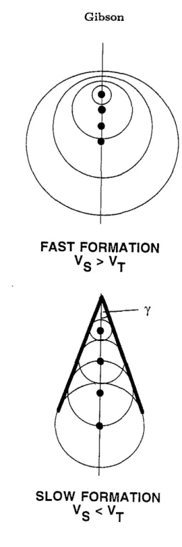
Data observed in crosshole seismic experiments often contain arrivals which are difficult to interpret, and the effects of the borehole on radiation of energy from down hole sources can be one important cause of these difficulties. In order to use the data from these experiments to infer properties of a petroleum reservoir, an improved knowledge of the effects of the borehole on the waves propagating in these experiments is therefore very useful. One difficulty which occurs during experiments conducted in some more shallow areas is the interpretation of the energy radiated from tube waves propagating in the source well. White and Sengbush (1963) noted this effect and suggested that large amplitude shear wave arrivals generated by an explosive source were the shear wave signals radiated from the tube wave propagating within the borehole. More recently, de Bruin and Huizer (1989) and Meredith (1990) confirmed that this effect can occur, and that the large amplitude and linear moveout of the shear signal in a receiver well is a feature typical of a Mach wave. Rutledge et al. (1992) also observed Mach waves in crosshole experiments conducted in the McKittrick oil field in California. These analyses and observations have shown that in slow formations, those where the tube wave velocity is larger than the formation shear wave velocity, the signals generated by the tube wave interfere constructively and build up a conical wavefront which has different geometrical spreading and travel time properties than the more typically observed spherical wave fronts propagating directly from source to receiver (Figure 1). In contrast, the energy from a tube wave in a fast formation does not interfere constructively and hence the tube wave signal is not observed at significant distances from the source well.

While standard discrete wavenumber and propagator matrix methods can be used to model these conical Mach waves in homogeneous formations where the source is in a cased or uncased well (Meredith, 1990), the problem becomes more difficult for a general layered medium such as is likely to be encountered in typical experiments. One approach to this general situation is to consider the tube wave to be a moving point source and then to compute the wavefields generated by that source by superposing the wavefields generated at each point along the well. Kurkjian et al. (1992) used this approach by developing an expression for the effective source at each point along the well using the equivalent source representation of Ben-Menahem and Kostek (1991) for an uncased well. A frequency-wavenumber domain algorithm was then used to compute the far-field waveforms. Simultaneously, Gibson (1992) developed a similar approach using ray methods to propagate the waves from the source well to receiver positions using a description of the moving source which allows a consideration of cased and cemented borehole models. Because numerous ray arrivals from each point along the source well were superposed, the method is called the Ray Summation Method (RSM). In this paper, I describe in detail the implementation of the RSM, which consists of several major steps. First, the group velocity of the tube wave is computed at each point in a discretized representation of the source well by differentiating the dispersion curve

of the tube wave. Secondly, the radiation properties of each individual point source are computed from the stress field generated by the propagating tube wave. Backus and Mulcahy (1977) have shown that such a stress field will act as a moment tensor source. Finally, rays are traced from receivers to each source point, which by applying the principal of reciprocity also yields the displacement fields corresponding to the waves propagating in the opposite directions. Su=ation of the wave fields from each source point, applying the appropriate delay times and source properties for the tube wave, then gives the shear and compressional wave fields generated by the tube wave. Following the description of this method, its accuracy is confirmed by a comparison to full waveform discrete wavenumber solutions for a homogeneous slow formation. Application of the RSM to a layered medium containing several slow formations shows complicated effects related to the reflection and refraction of Mach waves at interfaces. Since the RSM can be applied to any earth model which can be modelled using ray tracing, it is a tool which can be very useful in understanding wave propagation when there are significant complications from the source borehole.

METHOD

The borehole model consists of a system of concentric cylindrical layers representing the borehole fluid, casing, cement, formation and possibly other layers (Figure 2). This is the same model which is generally applied in full waveform acoustic logging studies and the properties of waves propagating within the borehole and the adjacent formation have been frequently studied (e.g., Cheng and Toks6z, 1981; White, 1983; Tubman et a!., 1984; Schmitt and Bouchon, 1985; Paillet and Cheng, 1991). Stationary phase radiation patterns for sources located in this borehole model can be computed using propagator matrix methods to solve the boundary condition equations at each of the interfaces (Gibson, 1993). However, these solutions are not applicable to a slow formation where the shear wave velocity is slower than the tube wave velocity (de Bruin and Huizer, 1989; Meredith, 1990). In this situation, the far-field amplitudes predicted by the approximate solutions become unrealistically large due to a vanishingly small term in the denominator of the radiation pattern equations (Lee and Balch, 1982; Meredith, 1990). The mathematical analysis breaks down because the tube wave pole approaches the stationary phase wavenumber in the complex plane, and the assumptions made in applying the stationary phase solution are no longer valid.

de Bruin and Huizer (1989) and Meredith (1990) showed that the influence of the tube wave can be understood physically as the generation of large amplitude conical waves due to constructive interference of the shear waves emitted by the tube wave as it propagates up and down the source well (Figure 1). This is directly analogous to the case of super-shear rupture in earthquake seismology (Ben-Menahem and Singh, 1981). While these waves are directly modeled by methods such as the discrete wavenumber

(1) technique in a homogeneous formation, the solution in an inhomogeneous medium is more difficult. A numerical solution for these media can be obtained by discretizing the source borehole along its length so that each point in the borehole becomes a point source which radiates energy when encountered by the tube wave (Figure 1). Ray tracing then yields the Green's tensor for wave propagation from each point in the source well to each receiver. The method is a discretized implementation of the following integral (Backus and Mulcahy, 1977; Ben-Menahem and Singh, 1981):

u(r,t)

=

J

dV(r')

J

dt' 8kG;j(r,t; r',t')Mjk(r',t')

whereGij(r,t;r',t') is a component of the Green's tensor yielding the ith component of

the displacement field at point r and time

t

due to a source acting along the jth coordi-nate direction at r' and t' (Aki and Richards, 1980). A moment tensor source component is indicated by Mjk(r',f). Similar methods have been applied to earthquake problems to simulate the displacement fields generated by complex source models (Cormier and Beroza, 1987; Spudich and Frazer, 1984). The fault is modeled as a two-dimensional surface of source points each of which emits energy at a given rupture time with a given slip mechanism. Hence, the borehole problem is actually somewhat easier in that only a line of source points need be considered. At the same time, it is complicated by the fact that the tube wave source will refiect up and down the borehole and each source point can emit energy several times.

Once a discretized representation of the source well is defined, the arrival time of the tube wave (the emission time of the source point) and the radiation pattern of the individual source points must be known in order to model the Mach waves. In order to compute the arrival time of the tube wave at a given source point, the group velocity of the tube wave must be known, and the stress field generated in the formation by the tube wave is required to compute the source radiation patterns. Backus and Mulcahy (1977) showed that a stress field acts as a moment tensor source such as Mij in Eq. 1. Since

the tube wave, or Stoneley wave, has also been analyzed in some detail (e.g., White, 1983; Kurkjian, 1985; Chang et a!., 1988; Cheng et a!., 1987; Norris, 1989; Paillet and Cheng, 1991), many of its properties are known and can be described analytically or numerically. These results 'can then be used to compute the necessary quantities as described below.

Source Time

Kurkjian (1985) presented a method to study individually the contributions of the var-ious waves in a borehole, including the tube wave. This approach is ideally suited to computation of the group velocity of the tube wave. The reflected pressure field in the borehole, the pressure field not including the direct arrivals from the source, can be written in the following form (Tsang and Rader, 1979; Cheng and Toksoz, 1981; and

others):

where PoRo is the amplitude of the source, w is angular frequency, X(w) is the ampli-tude spectrum of the source, Jo is the zeroth order Bessel function, k is the vertical wavenumber and kr

=

w2

I

a} - k2 is the radial wavenumber. Acoustic wave velocity in

the fluid is af, and Af(k,w) is a boundary condition coefficient. This coefficient Af has the general form

Af(k ) = Nf(k,w)

,w D(k,w) , (3)

and the denominator term is zero at the frequency-wavenumber pair corresponding to the tube wave pole. Kurkjian (1985) showed that the wavenumber at a given frequency can be found by locating the zeros ofD(k,w) using the Newton-Raphson method. This method uses the partial derivative ofD(k, w) with respect to k to perform an iterative search for the value giving D(k,w) = O. By locating the zeros corresponding to the pole kpole for specified values ofw, phase velocity c can be computed as a function of

frequency using c

=

wlk (Cheng and Toks6z, 1981). Then, the group velocity v is estimated from v = c

+

k

del

dk. This procedure is performed for all formations in the earth model. In general, Af(k,w) and D(k,w) are computed using propagator matrix methods to take into account the layers of cement and casing between the borehole fluid and the formation (Tubman et aI., 1984). Therefore, the group velocity found using this numerical approach will be the velocity appropriate for the well conditions of interest.

Radiation Properties

Backus and Mulcahy (1977) demonstrated that a stress anomaly (Jij acting in an

inho-mogeneous, elastic medium will act as a general moment tensor type source Mij . In

other words,

o-=M, (4)

where 0- is the anomalous stress tensor and M is the equivalent moment tensor source.

The stress field generated by the tube wave propagating up and down the borehole creates a local stress anomaly, and this stress anomaly relates the moving point source to a moving moment tensor. Kurkjian et al. (1992) make use of a similar idea in describing the tube wave in an uncased well as a sum of a moving isotropic, explosion-like moment tensor plus a vertical dipole.

Since in general the source borehole is likely to be cased and cemented, a more general description of the source is useful. This can be obtained numerically by computing the

stress field generated by the tube wave. First note that the displacement fields in the formation outside the borehole in terms of potentials 4> and

t/J

are (Paillet and Cheng, 1991): (5) uz(r,t) 84> 8'lj;

-8r 8r 84> 18r'lj;

+

-8z r 8r (6) (7) The radial and vertical components of displacement are u(r,t) and v(r,t), respectively, and the unit basis vectors in the rand

z

directions are

e

_{r and}

e

_{z. The general solutions} for these potentials in the formation can be written (Tsang and Rader, 1979; Cheng and Toksoz, 1981; Paillet and Cheng, 1991)

4> = [AnKo(lnr)]ei(kz-wt)

'lj; [EnKl (mnr)Jei(kz-wt).

Solution of the boundary condition equations at each of the interfaces between the formation and the fluid yields the coefficients An and En. These equations are solved easily and accurately using propagator matrix methods, the same procedure used to compute displacement fields in acoustic logging (Tubman et aI., 1984; Schmitt and Bouchon, 1985).

These components of the displacement field also describe the stress field. In cylindri-cal coordinates, assuming symmetry about the verticylindri-cal axis, the stress tensor is written (Ben-Menahem and Singh, 1981)

T

= (8)

The Lame parameters of the formation are given by

>.

and J1" and the basis vector for the ecoordinate is eO' Individual components Tijof the stress tensor are straightforwardly

derived using Eq. 8 and are presented in Appendix A.

In order to have a moment tensor source which is useful for the ray tracing, however, several additional operations must be performed on the tensor T to produce the desired moment tensor M. First, it must be converted to the Cartesian coordinates used for

the ray tracing algorithm. For a given value ofr,0,z, the basis vectors can be expressed in terms of the Cartesian basis vectors

ex, ey, ez

(Ben-Menahem and Singh, 1981):

e

r =

ex

cos0

+

ey

sinO

ee

-ex

sinO

+

ey

cosO (9)

ez

€z.

For example, the component Txx(O), corresponding to a given direction 0, is simply all terms multiplying the dyadic

exex:

(10) Once each of the tensor components is obtained in Cartesian coordinates, it must be integrated around the borehole surface in order to take into account the fact that the tube wave is radiating energy in all directions simultaneously. Since half of the borehole surface is "hidden" from the receiver and only radiates energy away from the receiver, the integration extends only over the other half of the borehole (Figure 3). The integration is also multiplied by the discretization interval t:>.z to take into account the extent of the source element along the borehole, and the result gives a component of the moment tensor M:

Mxx t:>.z

fa"

Trrcos20

+

Toosin2OdO

7r

= t:>.z2"(Trr

+

Too). (11) The total stress tensor M is derived by applying this procedure to all components of the stress tensor:

[

t:>.z~(Trr+TOO)

0

0]

M(k,w)

=

0 t:>.z~(Trr+Too) 0 .

o

0 t:>.z7rTzz

(12)

This moment tensor has the same general form as the explicit result obtained by Ben-Menahem and Kostek (1991) for a volume injection source in an uncased well. Kurkjian et al. (1992) applied this result to model the propagating tube wave as a moving volume source. Eq. 12 is more general in that it allows consideration of cased and cemented wells.

This moment tensor result is still a function of frequency and wavenumber, including the effects of all borehole waves, and the contribution of the tube wave must be isolated for application to the RSM. Just as the contribution to the displacement field by the tube wave can be isolated (Kurkjian, 1985), the stress field generated by the tube wave can be computed using the calculus of residues. Since the coefficients An and En appearing in the displacement and stress equations have the same denominator as does AII, the

appropriate tube wave pole kpole is located dUring the velocity estimation procedure. This approach locates the complexvalue of the pole, so that the imaginary part of this wavenumber can be used to estimate the attenuation of the tube wave as it propagates along the borehole via the term e-Im{kPOi,}z. The resulting stress fields at frequencyWo

are

Trr = 21rieiwt RAn [pe(2.B2 - c2)Ko(lr)

+

2P.B2~Kl(lr)]

+

21rieiwtREn _[ikm2P.B2(Ko(mr)

+

~

K1(mr))] e-1m{kP°i,}z Too - 21rie,wtRAn [-),

~:Ko(lr)

-

21'~Kl(lr)]

+

21rieiwtREn

[-i2P.B2~Kl(mr)]

(13) Tzz 21rieiwtRAn

[e

Ko(lr)

(),(1-

~)

-

p(2) ]

+

21rieiw

'R

En [-2ikmp.B2Ko(mr)] e-Im{kPOi,}z,

where the residues corresponding to the coefficients An and En, RAn and REn respec-tively, are

=

=

{ _{27rOD(k,w)/ok}I NAn e

ikZ}1

_{z k=kpoi,}

{ I NE

n

ikZ}1

27rOD(k,w)/oke z k=kPOi,'

(14)

The terms NAn and NEn are the numerators in the expressions for the two coefficient terms. They can be determined using the propagator matrix algorithm outlined by Tubman et al. (1984) Eqs. 13 are substituted into Eqs. 12 for each point along the discretized well.

Ray

Tracing

The travel times, amplitudes and polarizations corresponding to waves propagating from each source point to each receiver location are calculated using the dynamic ray tracing method (Cerveny, 1985). For a broad class of media conforming to the assumptions of ray theory, the high frequency asymptotic Green's tensor is completely determined by these quantities. The most important aspect of these assumptions is that the character-istic scale length of the medium is much longer than the wavelength of the propagating signal (Ben-Menahem and Beydoun, 1985). This allows the possibility of considering

the propagation of Mach waves in very general types of media, including layered earth models as well as models containing lateral heterogeneity (Ben-Menahem et aI., 1991; Cerveny et a\., 1987). Once the Green's tensor G(r,

t;r',

tI) representing displacement fields observed at r and time

t

due to a source operating at r' at source time

t'

is known, the displacement field generated by a moment tensor source is easily computed using Eq. 1. It is therefore straightforward to include the effects of the moment tensor of Eq. 12 in the simulation.

When the dynamic ray tracing is implemented for the RSM, the computational speed can be greatly increased by applying the paraxial method to extrapolate travel time and amplitude information from a given traced ray to nearby observation points (Cerveny, 1985). This method is advantageous because it eliminates the need to find individual rays exactly connecting every source/receiver pair. As another practical matter, it is more efficient to trace rays from receiver positions to the source positions than to trace them from sources to receivers, since there are in general fewer receivers than source points. The reciprocity of seismic wave propagation then can be used to relate the Green's tensors to the tensors for the reversed direction of propagation (Aki and Richards, 1980).

Summary of the Method

The implementation of the method can be summarized as follows:

1. Specify the earth model and the discretization of the source borehole.

2. For each point the source borehole, locate the tube wave pole for the dominant frequency of the source signal. Use this pole to compute the group velocity of the tube wave and arrival time at each point in the source hole.

3. Use the tube wave pole to compute the stress amplitudes at the source points using Eqs. 12 and 13. Include the attenuation of the tube wave.

4. Compute Green's tensors for waves propagating from each source point to the receivers. Sum the arrivals from all sources to each receiver with the appropriate time delays for the tube wave propagation, applying the moment tensors to the results. This is equivalent to evaluating the integral 1 via a discretization.

Each step of this method is relatively straightforward and all are relatively rapid compu-tational procedures. Some experimentation and comparison with full waveform solutions shows that the discretization interval D.z applied to the source well must be small e-nough to include at least five source points per shear wavelength. As long as the interval is this small or smaller, the discrete approximation to Eq. 1 will be accurate.

Note also that the effects of the reflection and transmission of the tube wave can be incorporated into the calculations. For example, a reflection of a tube wave from the free surface can be modeled by repeating step 2 in the procedure above to recompute the travel times of a tube wave originating at the free surface instead of at the actual borehole source location. Since the amplitude of the reflected tube wave will include a reflection coefficient of -1, all amplitudes of the Mach wave arrivals must be multiplied by this factor. The reflections from other interfaces can be included in a similar fashion. An estimate of the appropriate reflection coefficients can be obtained from the low frequency expressions derived by White (1983). The transmission coefficients can also be obtained from these equations, allowing an approximate inclusion of the reduction in amplitude of the tube wave when it traverses an interface.

NUMERlCAL RESULTS

Homogeneous Medium

In order to demonstrate the validity and accuracy of the RSM, consider first a homoge-neous model with the velocities and density of the Pierre shale (White and Sengbush, 1963). These parameters are a

=

2074

mis,

/3

=

869

mls

and

p

=

2.25

g/cm

3

• Fluid

velocity was set to 1500

mis,

with density 1.0

g/cm

3_{, and the borehole model included}

casing and cement. The dimensions of this borehole model and velocities of the steel casing and cement are shown in Table 1.

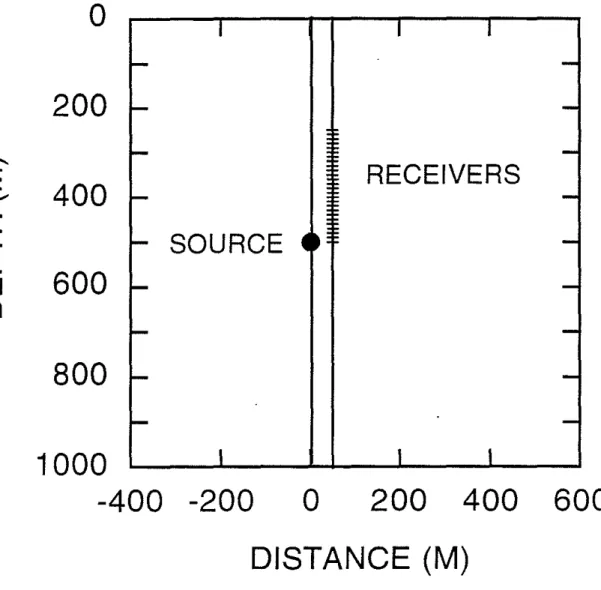
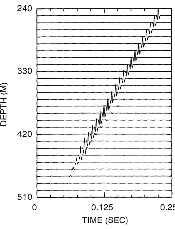
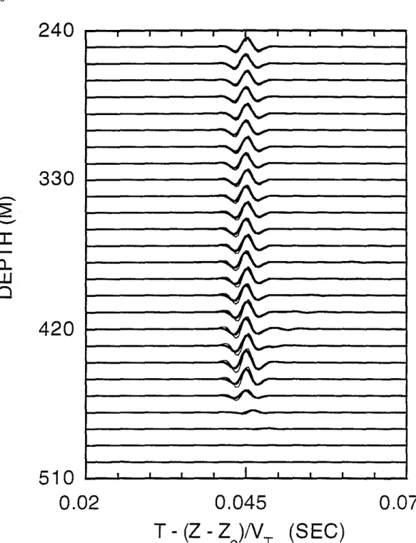
Calculations were performed using the discrete wavenumber method (Bouchon and Aki, 1977; Bouchon, 1980; Tubman et aI., 1984; Meredith, 1990) and the RSM for a model with boreholes separated by 50 m, a source at depth 500 m and 26 receivers located every 10 m in depth from 500 m to 250 m (Figure 4). Since the modeling methods considered here do not consider the effects of the receiver borehole on synthetic seismograms, the computational results are for an idealized experiment with receivers perfectly coupled to the formation. A volume point source was applied, and a 200 Hz Ricker wavelet was used as a source wavelet. Since the group velocity of the tube wave at 200 Hz in a cased well, 1384

mis,

is faster than the shear velocity, a borehole source will generate a Mach wave in this medium. In Figure 5, the radial component RSM synthetic seismograms are shown for this configuration. The Mach wave dominates the seismograms and displays a very large amplitude signal with a linear moveout velocity for receivers above about 440 m in depth. In contrast, the P wave generated by the primary vol ume injection source is almost undetectable on the scale of this figure, arriving at about 0.025 s for the receiver at 500 m. The generation of the Mach wave is easily understood by examining the shear wavefronts generated by the propagating tube wave. Figure 6 displays the wavefronts generated by a subset of the point sources at a time of 0.30 sec after the volume source was activated. These spherical wavefronts interfere

constructively along conical wavefronts above and below the primary source location, and the angle between this conical wavefront and the vertical is controlled by the velocity difference between the tube wave and the shear waves in the medium (Ben-Menahem and Singh, 1981; Meredith, 1990). This angle (-y in Figure 1) is given by sin'Y

=

f3/V"

where

f3

is the formation S-wave velocity and V, is the tube wave velocity. A faster shear wave velocity would therefore yield a Mach wavefront propagating closer to perpendicular to the borehole.

The discrete wavenumber and RSM results are compared in Figure 7. A P-wave ra-diation pattern was computed using the generalized stationary phase solution (Gibson, 1993), and the ray results, both P and S-wave, were normalized so that the P-wave sig-nals at the 500 m receiver had the same amplitude as the discrete wavenumber synthetic seismogram. The normalization factor is required due to some differences in the way the two computer routines scale FFT computations. It is clear from these results that the RSM synthetic seismograms are very close to the full waveform discrete wavenum-ber solution, and that the RSM algorithm is able to accurately compute the wavefield generated by the tube wave. There are some subtle differences in the predictions of the two methods, but the RSM yields the same travel time and the same general wavelet shapes as the discrete wavenumber method.

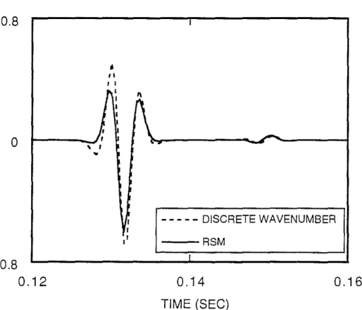
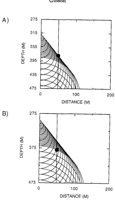
Comparison of the results for an individual trace helps to' clarify these comments, In Figure 8, the synthetic seismograms for the receiver at 380 m are displayed for a time window containing the Mach wave arrival. It can be seen that though the RSM result is slightly low in overall amplitude, it predicts the shape of the Mach wavelet very well. For both results, the first positive peak is slightly larger than the second. In addition, this display makes obvious a second arrival arriving at about 0,15 sec. A close examination of the complete synthetic seismogram in Figure 5 shows this weaker signal trailing the Mach wave by increasingly large time lags. This second event is easily explained by examining shear wavefront plots. In Figure 6, the spherical wavefronts emanating from each individual point source are very densely spaced in a roughly triangular region between the leading edge Mach wave front, which is conical in the complete three-dimensional picture, and a trailing wavefront which is slightly curved. A close examination of wavefront plots at the arrival times of the two signals in Figure 8 shows the relationship of the waves to the dense energy band. At the arrival time of the Mach wave, 0.132 sec, the conical wavefront has traveled to the receiver (Figure 9A). In contrast, at 0.15 sec, the trailing edge of the closely spaced wavefronts is at the receiver location (Figure 9B). Between the conical front edge of the energy packet and this trailing edge, the arrivals at the receiver tend to cancel out since peaks overlay troughs. However, there are nonzero contributions to the total wavefield from both the leading and trailing edges of the energy packet. It can also be shown that the last wavefront in the energy band, the trailing edge, corresponds to the wavefront originating from the primary source at time

t

=

0, and thus this second shear wave is arriving at the normal shear wave time. In this case, the RSM solution helps to interpret

an arrival which would be difficult to understand given only the discrete wavenumber results.

It is important that the RSM is able to predict the wavelet shape for both of the shear wave arrivals, since both display phase shifts relative to the normal far field radiation from a borehoie source. In particular, the P and S-wave signals in the typical fast formation have a time response proportional to the time derivative of the source pulse (Lee and Balch, 1982; Meredith, 1990). Here we see, however, that the Mach wave arrival is approximately proportional to the source Ricker wavelet multiplied by-1. The integration of the many shear wavefronts emitted by the individual point sources results in another change in phase of the far-field Mach wave signal. The S-wave at 0.15 sec in Figure 8 is proportional to the time derivative of the Ricker wavelet multiplied by -1.

The presence of casing in the source well has a large effect on the Mach waves signals. First of all, the tube'velocity is significantly larger in a cased well. When the 10 em radius borehole in the Pierre shale is uncased, the tube wave group velocity at 200 Hz is 962

mis,

instead of the 1384

mls

velocity for the cased well model. This will change the moveout velocity of the Mach wave also, as well as its angle of propagation (Meredith, 1990). Just as important as this velocity effect, however, is the dispersion of the tube wave, which is negligible over the frequency range of importance for a 200 Hz Ricker wavelet in the cased well, but is significant in the uncased well. The synthetic seismograms for the uncased well in Figure 10 demonstrate this effect. Whereas the RSM solution predicts the waveform of the Mach wave at all depths for the cased well model (Figure 7), there are significant differences in waveforms between the RSM and discrete wavenumber results at depths far from the source when the well is uncased. This is because the dispersion of the tube wave causes a difference in the shape of the source wavelet at each point along the discretized source well. In essence, each frequency arrives at the individual point sources at slightly different times. Another important effect of the casing is that it reduces the amplitude of the Mach waves by a factor of about 2 so that the galn applied to the synthetic seismograms for the cased well (Figure 7) is twice the gain applied to the results from the uncased well (Figure 10). The amplitude of the P-wave radiated by the source will also be significantly reduced by the casing in slow formations such as the Pierre shale (Gibson, 1993). In principle, the RSM could be formulated to take the dispersion into account by recomputing the summations of ray theoretical wavefields for each frequency, since the ray paths, travel times and amplitudes are independent of frequency. Only the point source times and amplitudes would change. Since most wells in shallow, soft formations will be cased, however, this effect is not likely to be important in most practical cases.

Layered Medium

Figure 11 shows a simple, three layer model with a source and receiver well which are 100 m apart. The source is located at a depth of 225 m, and receivers are located every 10 m from 10 to 400 m in depth. All three layers have low velocities, so that Mach waves can be expected to be generated in each layer. Shear wavefronts from the source at an elapsed time of 0.3 sec show the complications introduced by the different layers (Figure 12). In the top layer, there are two Mach waves present, one generated by the tube wave in this layer, and another which was generated in the middle layer and which has been transmitted into the first layer. Each wavefront contributing to this composite figure will obey Snell's law at the interface and so will the conical wave. Since the velocity in the top layer is lower than the velocities in the middle layer, the angle between the two Mach waves creates a sharp corner. There are also two Mach waves in the bottom layer, but in this case the velocity increase across the interface has resulted in a rounded corner between the conical waves. This is because the Mach wavefront refracts to travel closer to a horizontal direction as it crosses the interface. The homogeneous Pierre shale model shows that two far-field shear wave signals were generated in the slow formation due to the edges of dense energy bands in the wavefront pictures. In Figure 12, there are several such energy bands created by the different layers, suggesting that in the presence of inhomogeneity, several different S-wave arrivals can be generated by the source, even neglecting the contributions of reflected energy.

A 100HzRicker wavelet was used as a source wavelet to compute synthetic seismo-grams for this model using a volume injection source. Reflections of the P-waves and the tube waves at each interface and at the free surface were included in the modeling. The radial component synthetic' seismogram shows the complications resulting from the layering (Figure 13). Several conclusions can be drawn from this result. First of all, because the top layer has very slow SandP-wave velocities, both P and S Mach waves are generated there, so that very strong P and S-wave signals are seen in the top few receivers. The P Mach wave is also reflected, and the reflected tube wave generates a down-going Mach wave in the first layer. Therefore, a late arriving, relatively strong P-wave can be seen arriving at around 0.45 sec. Itcan also be seen that the shear Mach wave is reflected, and the down-going reflected tube wave generates the largest signals. In contrast, the effects of the intermediate interfaces are relatively weak.

CONCLUSIONS

The Ray Summation Method provides a useful means of studying the radiation by tube waves of both shear and compressional wave energy into formations surrounding the borehole. By modeling the tube wave as a moving point source, it is possible to synthesize the far-field conical Mach waves which are observed in formations of slow

velocity (e.g., de Bruin and Huizer, 1989). Because the tube wave velocity and the stress anomaly which determines the moment tensors at each point source are determined numerically using a concentrically layered model of the borehole, it is possible to consider both open and cased, cemented boreholes with the RSM. The use of ray tracing to compute the far-field shear or compressional waves arriving at the receiver locations from each point source also allows the consideration of inhomogeneous, laterally varying earth models. The accuracy of the RSM was demonstrated by a comparison with discrete wavenumber results for a homogeneous, slow formation. In addition, this comparison confirmed that the RSM accurately predicts the presence of two shear waves in slow formations: the Mach wave and a weaker S-wave arriving at the normal body wave travel time.

Synthetic seismograms for a layered earth model illustrate the complications in seis-mic wave observations which can be caused· by inhomogeneity in combination with the radiation of energy by the tube wave. Each time the tube traverses an interface with a significant velocity contrast, the conical wave generated in the formation containing the incident tube wave is refracted across the interface according to Snell's law. In addition, a new Mach wave, oriented at a different angle with respect to the vertical, is generated in the formation containing the transmitted tube wave. Because the tube wave is completely reflected at the free surface, there are also large amplitude Mach waves associated with the down-going energy. This will create large amplitude signals later in the seismic section. Since one layer, the most shallow, had a very slow compres-sional wave velocity as well as a low shear wave velocity, a comprescompres-sional Mach wave was generated in addition to the more typical shear conical wave.

A by product of the use of ray tracing in computing the RSM synthetic seismograms is the ability to compute wavefront plots at different points in time after the tube wave is created by the primary source. In a homogeneous formation, these figures show clearly how a conical wave forms. More importantly, in an inhomogeneous medium, the wavefront plots help to better understand the many arrivals which are present in the synthetic seismograms. With the aid of these figures, the relative geometry of the different conical wavefronts is explained. By combining a simple, intuitive model of the tube wave, the moving point source, with the flexible and rapid dynamic ray tracing algorithm, the RSM is a means of both simulating and better understanding borehole source behavior in slow formations.

ACKNOWLEDGEMENTS

This work was supported by Societe Nationale Elf Aquitaine (P) as a post-doctoral fellowship at the Universite Joseph Fourier, Grenoble, France. Additional funding was provided by a Founding Member Post-doctoral fellowship at the Earth Resources Lab-oratory, Massachusetts Institute of Technology. I would like to thank Drs. J .-L. Boelle, M. Bouchon and C.R. Cheng for helpful discussions regarding the nature of conical waves and tube wave propagation.

REFERENCES

Abramowitz, M., and Stegun, I., 1964, Handbook of Mathematical functions with

For-mulas, Graphs and Mathematical Tables, Dover.

Aki, K., and Richards, P.G., 1980, Quantitative Seismology, Theory and Methods, vol. 1, W.H. Freeman and Company, San Francisco.

Austin, E.H., 1983, Drilling Engineering Handbook: International Human Resources Development Corporation, Boston.

Backus, G., and Mulcahy, M., 1977, Moment tensors and other phenomenological de-scriptions of seismic sources-I. Continuous displacements: Geophys. J. R. Astr. Soc.,

46,

341-361.

Ben-Menahem, A., and Singh, S.J., 1981, Seismic Waves and Sources, Springer-Verlag, New York.

Ben-Menahem, A., and Beydoun, W.B., 1985, Range of validity of seismic ray and beam methods in general inhomogeneous media-I. General theory, Geophysics, 82, 207-234.

Ben-Menahem, A., and Kostek, S., 1991, The equivalent force system of a monopole source in a fluid-filled open borehole, Geophysics, 56, 1477-1481.

Ben-Menahem, A., Gibson, Jr., R.L., and Sena, A.G., 1991, Green's tensor and radia-tion patterns of point sources in general anisotropic inhomogeneous elastic media,

Geophys. J. Int., 107, 297-308.

Bouchon, M., 1980, Calculation of complete seismograms for an explosive source in a layered medium, Geophysics,

45,

197-203.

Bouchon, M., and Aki, K., 1977, Discrete wavenumber representation of seismic-source wave fields, Bull. Seis. Soc. Amer., 67, 259--277.

Cerveny, V., 1985, The application of ray tracing to the propagation of shear waves in complex media, in Seismic Shear Waves, Part A: Theory, Dohr, G.P., Ed., in, Handbook of Geophysical Exploration, Helbig, K., and Treitel, S., Eds., Section 1: Seismic Exploration, 15A, Geophysical Press.

Cerveny, V., Pleinerova., J., Klimes, L. and Psencik,1., 1987, High-frequency radiation from earthquake sources in laterally varying layered structures, Geophys. J. R. Astr. Soc, 88, 43-79.

Chang, S.K., Liu, H.L., and Johnson, D.L., 1988, Low-frequency tube waves in perme-able rocks, Geophyics, 53, 519-527.

Cheng, C.H., and Toksoz, M.N., 1981, Elastic wave propagation in a fluid-filled borehole and synthetic acoustic logs, Geophysics,

46,

1042-1053.

Cheng, C.H., Zhang, J., and Burns, D.R., 1987, Effects of in-situ permeability on the propagation of Stoneley (tube) waves in a borehole, Geophysics, 52, 1279-1289. Cormier, V., and Beroza, G., 1987, Calculation of strong ground motion due to an

extended earthquake source in a laterally varying structure, Bull. Seis. Soc. Amer.,

77, 1-13.

de Bruin, J., and HUizer, W., 1989, Radiation from waves in boreholes, Scientific

Drilling, 1, 3-10.

Gibson, Jr., R.L., 1992, Models of seismic wave radiation from borehole sources in fast and slow formations: 62nd Ann. Internat. Mtg., Soc. Expl. Geophys., Expanded Abstracts, 133-136.

Gibson, Jr., R.L., 1993. Radiation from seismic sources in cased and cemented boreholes:

submitted to Geophysics.

Kurkjian, A.L., 1985, Numerical computation of individual far-field arrivals excited by an acoustic source in a borehole, Geophysics, 50, 852-866.

Kurkjian, A.L., Schmidt, H., Marzetta, T.L., White, J.E., and Chouzenoux, C., 1992, Numerical modeling of cross-well seismic monopole sensor data: 62nd Ann. Internat. Mtg., Soc. Expl. Geophys., Expanded Abstracts, 141-144.

Lee, M., and Balch, A., 1982, Theoretical seismic wave radiation from a fluid-filled borehole, Geophysics, 47, 1308-1314.

Meredith, J., 1990, Numerical and analytical modelling of downhole seismic sources: the near and far field: Ph.D. thesis, Massachusetts Institute of Technology.

Geophysics, 54, 330--341.

Paillet, F.L., and Cheng, C.H., 1991, Acoustic Waves in Boreholes, CRC Press, London. Press, F., 1966, Seismic velocities, in Clark, J.S., Ed., GSA Memoir 97: Handbook of

Physical Constants: Geo!. Soc. Amer.

Rutledge, J.T., Albright, J.N., Phillips, W.S., Fehler, M.C. and Howlett, D.L., 1992, Observation of Mach waves at the McKittrick oil field: 62nd Ann. Internat. Mtg., Soc. Expl. Geophys., Expanded Abstracts, 151-154.

Schmitt, D., and Bouchon, M., 1985, Full-wave acoustic logging: synthetic microseismo-grams and frequency- wavenumb~r analysis, Geophysics, 50, 1756-1778.

Spudich, P., and L.N. Frazer, 1984, Use of ray theory to calculate high-frequency radi-ation from earthquake sources having spatially variable rupture velocity and stress drop, Bull. Seis. Soc. Amer., 74,2061-2082.

Tsang, L., and Rader, D., 1979, Numerical evaluation of transient acoustic waveform due to a point source in a fluid-filled borehole, Geophysics, 44, 1706-1720.

Tubman, K.M., Cheng, C.H., and Toksoz, M.N., 1984, Synthetic full waveform acoustic logs in cased boreholes, Geophysics, 4g, 1051-1059.

White, J., 1983, Underground Sound: Application of Seismic Waves, Elsevier.

White, J., and Sengbush, R., 1963, Shear waves from explosive sources, Geophysics, 28, 1101-1119.

APPENDIX A

THE STRESS TENSOR INDUCED BY BOREHOLE WAVE

PROPAGATION

A complete characterization of the stress field in the formation associated with the propagation of borehole waves requires a specification of four different components of the stress tensor in the cylindrically symmetric system (Eq. 8). Derivation of these components using Eqs. 6, 7, and 8 is straightforward, and the results are:

Trr(k,w)

=

An

[pnk2(2,B~

- c2)Ko(lr)

+

2P~;'1

K1(lr)] +En

[ikm2Pn,B~

( Ko(mr)

+

~r

K 1(mr») ] Trz(k,w) An[-i2Pn,B~kIK1(lr)]

+

En[pe(2,B~-

c

2)K1(mr)]

Too(k,w) = An [

-~r2

Ko(lr) -

2~nl

K1(lr)]

+

En

[-i2P;,B~k

Kl(mr)]

Tzz(k,w) = An {k2[An

(1-

~~)

-

pna~]

KO(lr)}

+En[-ikm2Pn,B~Ko(mr)]. (AI)

A common factor eik(z-ct) has been suppressed in each of these equations. In each of

the terms involved in these stress tensor components, the suffix

n

indicates that the quantity is evaluated in the formation, the nth layer of the borehole model (Figure 2). The ,Bn, an, and Pn are S-wave velocity, 'P-wave velocity and density, respectively, and

( C2 ) 1/2 I = k 1 -a2 n ( c2 ) 1/2 m = k 1 - ,B;' (A2)

In addition, k is the vertical wavenumber, k

=

w/c, and Ko(z) and K1(Z) are modified Bessel functions. Derivation of the stress component equations is simplified by using the expressions given by Abramowitz and Stegun (1964) for the derivatives of the modified Bessel functions.

In order to completely evaluate the stress field, the boundary condition constants Anand En must also be known. They can be determined by the same procedure which Tubman et al. (1984) apply to the computation of analogous constant for the borehole fluid. Using propagator matrices to solve the boundary conditions at each interface in the borehole model (Figure 2) between fluid and formation is a fast and accurate way to determine these constants (Schmitt and Bouchon, 1985).

I

Layer

I

Outer radius (cm)

I

P-wave velocity

I

S-wave velocity

I

Density

I

Fluid 7.6 1500 m/s

o

m/s 1.0 g/cmo

Casing 8.9 5940 3228 6.268

Cement 10.0 3175 1833 1.92

Table 1. Physical properties of the borehole model. The borehole model considers a typical 20 cm (77/8 in) borehole, with a casing of outer diameter 17.8 cm (7 in) and inner diameter 15.2 cm (6.004 in). Water was used as the borehole fluid for all computations. Velocities of the Solenhofen limestone and steel and the density of the limestone are from Press (1966), and the density of steel is obtained from Austin (1983).

FAST FORMATION

V

_s

>

V_T

SLOW FORMATION

V

_s

<

V

T

Figure 1: Schematic diagram of radiation from propagating tube waves. A) Fast formation. No Mach wave is generated. B) Slow formation. Constructive interference of shear wave fronts in the formation creates a conical Mach wave. The size of the angle 'Y between the conical wavefront and the vertical is determined by the contrast between formation shear wave velocity and tube velocity. This angle is given by sin'Y

=

l3/lIt,

where

13

is the formation shear wave velocity and

lit

is the tube wave velocity.

Figure 2: Cross section of a borehole model. The layers are numbered 1 ton, where 1 is the borehole fluid and n is the formation. Interfaces between the concentric layers are labeled as indicated.

y

z

x

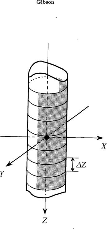
Figure 3: Schematic diagram illustrating the discretized borehole model and the region of the borehole wall over which the stresses are integrated to compute the ef-fective moment tensor sources (equation eq:momten). The region shaded is the region appropriate for a receiver located in the x - z plane, where x

>

o.

600

400

200

o

I

I

I

-

--

--

::

-RECEIVERS

f-

-SOURCE 4

E

-

~

--

--

--

-f-

-I I I

o

200

800

1000

-400 -200

- .

~

400

I

I-fu

600

o

DISTANCE (M)

Figure 4: Source and receiver configurations for a homogeneous Pierre shale model. There are 25 receivers between 250 m and 500 m in depth. The formation properties are described in the text, and properties of the cased borehole model are given in Table 1.

0.25

0.125

TIME (SEC)

•

•

I I I I I _• ~ ~

vr

~

yv

pv

1"

IVv

ft

yv

ft

vv

ft

vv

[W-Ilv

!

vv

W

IV

P

/V

II

Ir I n

.

I I

•

• I

•

• I

•

510

o

240

330

-

~

--I

f-a..

W

0

420

Figure 5: Radial component RSM synthetic seismogram for the homogeneous Pierre shale model with a cased well (Figure 4). The P wave is barely visible at depth 500 m, time 0.25 sec. The strongest signal is the Mach wave.

o

-

2

--

I

I-CL

W

o

200

400

600

800

SOURCE

1000

-400

-200

o

200

400

600

DISTANCE (M)

Figure 6: Shear wavefront diagram at time 0.30 sec, when the source is located in a cased borehole. This figure shows only the wavefronts propagating towards the right for clarity, and the complete figure is symmetric about the source borehole.

0.07

0.045

T -

(Z -

Zo)N

T

(SEC)

I I I I

A '

I I I

....,

...

....,

...

....,

....

....,

...

....,

....

--

....,

...

...

....,

...

-,

....

vI\...

vI\...

~

...

...

,

...

~I\""

-VI\.'"

~

_~t\

"'YJ"v

_"<'Iv

""'"

•

I I • I ,

•

I

•

510

0.02

240

330

.-.

~

--

I

I-0..

W

0

420

Figure 7: Overlay of the radial component RSM synthetic seismograms (bold line) and the discrete wavenumber results (fine line) in the homogeneous Pierre shale model with a cased well. The seismograms were plotted with a reduction velocity equal to the tube wave group velocity in order to emphasize this waveform. The two solutions are very similar, confirming the accuracy of the RSM approach.

0.16

0.14

TIME (SEC) I

•

"

~~

~

,

,,

•

I

-, I

-¥ I - - - DISCRETE WAVENUMBER I " RSM I

o

0.8 -0.8

0.12

Figure 8: Overlay of the traces corresponding to the receiver at depth 380 m (Fig-ure 4). These seismograms were computed using a cased source well model. Note especially the smaller shear wave arrival at about 0.15 sec.

( 200 100 DISTANCE (M) 475

o

~ ~ 375 0-w o

A)

275 315 ~ 355 I fo- 0-w ₃₉₅ 0 435 475 0 100 ₂₀₀ DISTANCE (M)

B)

275

Figure 9: Shear wavefront diagrams explaining the origin of the two arrivals seen in the traces in Figure 8. (A) This diagram is for time 0.132 sec, and shows the arrival of the conical wave at the receiver. (B) This diagram, for time 0.15 sec, shows the origin of the secondary shear wave. At this time, the wavefront by the point source coincident with the primary volume injection source is at the receiver. The wavelets from the other closely spaced wavefronts in the region between the conical wavefront and this latter wavefront cancel out in the summation since peaks tend to overlay troughs. Note that for clarity this figure shows only a subset of the wavefronts that were actually summed in the computation of the RSM synthetic seismograms.

•

:c

f-a..

ill

o

240

330

420

. rA"\.,.:;...'

' __

' __

-I

-~

t---...,,""'"'A:l

,yo'v"''''---1

t-

....,,~.~'O' "'itl1:f

-..1'-,\!:l"wP---l

_ V

1 - - - _

..

J

_'I\\!/'---1

J - - - "

J

\\1,'1"'-

--1

t - - -

~ ~r---I

1--

~.:l~\.,.':1.---1

"i7,,'-""

-1

~A

.

510

o

.

, , I

0.025

T -

(2 - 2

)N

o

T

. .

(SEC)

0.05

Figure 10: Overlay of the RSM (bold line) and discrete wavenumber (fine line). synthetic seismograms in the homogeneous Pierre shale model when the source well is uncased. This figure shows the radial component of displacement. Now the dispersion of the tube wave in the source hole causes a dispersive effect of the Mach wave as well whicb is not correctly modeled by the RSM. This could be taken into account by applying a frequency varying form of the algorithm.

250

RECEIVER

WELL

,

-50

50

150

DISTANCE (M)

SOURCE

WELL

,

I I I

Vp=1 000

V

_S

=500

(m/s)

-

-I-

-4

t

Vp=1500

V

_S

=750

-

-Vp=1550

_VS=850

I I I

400

-150

o

100

300

~

200

0...

W

o

Figure 11: Layered earth model with source and receiver wells 100 m apart. The P and S-wave velocities of each layer are indicated in the figure. There are a total of 40 receivers at an interval of 10 m.

o

100

.

-2

-

_~

200

0-LU

o

300

400

-150

-50

50

150

DISTANCE (M)

250

Figure 12: Shear wavefront diagram at 0.30 sec. This figure demonstrates some of the complications in conical wave propagation which will occur in layered media. The conical waves are refracted on traversing each interface.

I'lt V1 "n" 't. 'T "A iii,

:ft

""

I-

-..

I.

S

I

P

!Vs

0.2

0.4

TIME (SEC)

o

105

--

2

--I

b:

210

u.J

o

315

420

o

p

s

0.6

Figure 13: Radial component RSM synthetic seismogram for the layered earth model (Figure 11). The letters "P" and "S" show the upgoing Mach waves arriving at the most shallow receiver. Likewise, at the bottom of the figure, the letters identify the corresponding downgoing conical waves.