Cavity and projectile dynamics in intermediate Froude number water entry

Cavity and projectile dynamics in intermediate

Froude number water entry

Jakub K. Kominiarczuk

Submitted to the Department of Physics in partial fulfillment of the requirement for the degree of

Bachelor of Science

Massachusetts Institute of Technology Cambridge, June 2007

©2oo7 Jakub K. Kominiarczuk

All rights reserved

The author hereby grants to MIT permission to reproduce and to distribute publicly paper and electronic copies of this thesis document in whole or in part in any medium

now known or hereafter created.

Author ... ... :..-...

Jakub K. Kominiarczuk Department of Physics May 22, 2007

Certified by ... .. /*

Professor Dick K. P. Yue Thesis Supervisor Department of Mechanical Engineering

Accepted by ... ,... ... Professor David E. Pritchard

Senior Thesis Coordinator

Department of Physics _{MASSACHUSETTS INS E}

OFTECHNOLOGY

AUG 0 6 2007

LIBRARIES

SUPERVISOR:

Quidquid agis,

prudenter agas

et respicefinem

ACKNOWLEDGMENTS

The author would like to sincerely thank Professor Dick K.

P. Yue for his guidance and mentoring during the progress

of this project. I am also grateful to Dr Kelli Hendrickson

for her help, mentoring, and friendliness that she always

showed when needed most. Additionally, the author is

indebted to the wider Vortical Flow Research Lab group,

especially to Grgur Tokic for his precious time spent at

explaining how fish swim, Tadd Truscott for the entire

summer spent at building the illumination system, and

Areti Kiara for the valuable time at the beginning of my

project.

The author owes gratitude to Anna Labno, who

con-stantly supported him and went through many storms

without a shade of hesitation.

Finally, the author is most indebted to his parents and

family who provided unwavering support throughout my

studies at MIT, providing a wider perspective and

encour-agement.

CONTENTS

1 INTRODUCTION 1

1.1 Water entry 1

1.2 Literature overview 2 1.3 Scope of the thesis 6

2 _{QUALITATIVE FEATURES OF WATER ENTRY} CAV-ITIES ₉

2.1 _{Description of a water entry 9}

2.2 Scaling laws and important parameters ₁₂

3 EXPERIMENTAL INVERSTIGATION 15 3.1 Experimental setup 15 3.2 Photographic techniques 17 3.3 Data analysis 21 3.3.1 Projectile tracking 22 3.3.2 Error analysis 28 3.4 Experimental results 32 3.4.1 Ball motion 32 3.4.2 Cavity shape 34 3.4.3 Deep closure 35 4 PROBLEM FORMULATION 39

4.1 Classical high Froude number approach 40 4.2 Slender body approach 44

4.2.1 Non-dimensional equations 52 4.2.2 Classical problem - small, high-speed

projectile 55

5 THEORETICAL MODELING 57

5.1 Governing equations 57

5.1.1 Dimension reduction 58

5.2 Numerical algorithm 60

Figure i Evolution of a cavity. One can easily

see the three important stages of wa-ter entry: (a) impact and splash for-mation, (b) cavity forfor-mation, and (c) deep closure. 2

Figure 2 Schematic view of a vertical water en-try after the closure of a dome-like structure atop the cavity. 1o

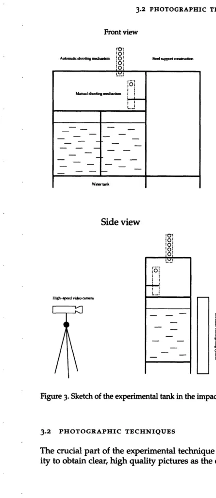
Figure 3 Sketch of the experimental tank in the impact laboratory. 17

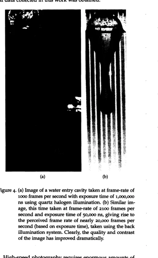
Figure 4 (a) Image of a water entry cavity taken at frame-rate of iooo frames per sec-ond with exposure time of ,000,000ooo ns using quartz halogen illumination. (b) Similar image, this time taken at frame-rate of 2100 frames per second and exposure time of 50,000 ns, giv-ing rise to the perceived frame rate of nearly 20,000 frames per second (based on exposure time), taken using the back illumination system. Clearly, the quality and contrast of the image has improved dramatically. 18

Figure 5 Design of the support rails for the back illumination system. 19

Figure 6 Transformation space of the linear Hough transform. The horizontal axis depicts distance d while the vertical one repre-sents the angle 0 between the line and the x-axis. The gray scale coding en-codes the number of pairs (d, 0) that fall within a given bin in the transfor-mation space. 24

List of Figures 7

Figure 7 Image tracking algorithm. (a) Origi-nal image; (b) Image after subtraction of the previous frame; (c) Sobel gra-dient detection; (d) Sphere of inter-est isolated on an image; (e) circular Hough transform applied to the im-age; (f) recovered position of the pro-jectile. 30

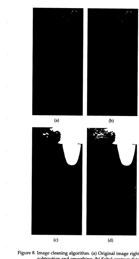
Figure 8 Image cleaning algorithm. (a) Origi-nal image right after subtraction and smoothing; (b) Sobel contour detec-tion; (c) image after localization of the main features; (d) image after the eat-and-grow clearing algorithm. As can be clearly seen, the cavity has been uniquely found and noise from the camera has been successfully removed. 31

Figure 9 _{Trajectories of four projectiles entering} water at different Froude numbers. (a)

Impact at F = 3.62, (b) impact at F = 4.40, (c) impact at F = 5.51, (d) impact at F = 6.47. 33

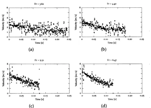
Figure io _{Velocities of the four projectiles} en-tering water at different Froude num-bers, corresponding to the trajectories from Fig. 9. Velocities were obtained by fitting lines to by selecting a mov-ing window of with of 15 points and defining the instantaneous velocity at the time corresponding to the center of the window as the slope of the fit-ted line. 34

Figure 1•1 _{Radius of the cavity R(z, t) for a} num-ber of instants of time. The points represent experimental data while the solid line is a polynomial fit to the data. The data series used for creation of this sequence was named Ballo200 and as one of the very few has been recorded before the engineering of the illumination system. 36

closure TdVo/Ro is shown to be lin-early dependent on Froude number, and a similar relation appears to hold in the case of the non-dimensional depth of the deep closure Zd / R0. For concrete data points in their dimen-sional form please consult the Table 2

in the Appendix A. 37

Figure 13 Two limiting situations showing the shape of the cavity for (a) the initial phase of water impact when the pro-jectile is only half-submerged and clearly only the potential due to the projectile counts, and (b) after a long time when the cavity becomes very long and thin with the potential of the cavity domi-nating the cavity dynamics. 45

LIST OF TABLES

Table -i Specification of the input format of for the projectile and cavity tracking program. 23

List of Tables 9

Table 2 _{Complete list of analyzed and usable}

data from the sets collected using the new back illumination. Each row con-tains the number of the run, its catalog name, initial velocity of the projectile, and the depth Zd and time Td of the deep closure. 61

LIST OF SYMBOLS USED

R0 Radius of projectile

v0 Initial velocity of projectile

Zd Depth of the deep closure

INTRODUCTION

1.1 WATER ENTRY

Water entry of projectiles has long been a topics of interest in both sciences and engineering. It began with Worthing-ton, who in the late XIX century found experimentally that a cavity is being formed when a steel sphere enters water (Worthington and Cole (1895-1896)). As we know today, water entry of a sphere is a complex process which nonethe-less can be enormously simplified, making it a particularly rewarding area of research.

During the impact, surface of the projectile becomes wet-ted which together with the form drag produce a drastic decrease in the projectile velocity. At this stage, the energy lost by the ball is transferred primarily into the splash, which takes a form of vertical sheet of water emerging from around the circumference. If the body is moving at a high enough velocity, the displaced fluid will not collapse imme-diately but rather expand the cavity formed behind it. The evolution phase is the longest of all, and is governed by a continuous energy transfer from the projectile into the fluid through the pressure field formed at the wetted surface. Cavity walls continue to expand at the cost of their kinetic energy which is transformed into potential energy asso-ciated with hydrostatic pressure in the surrounding fluid. Inevitably, after all the kinetic energy is used for expand-ing the cavity the wall velocity reverses and causes rapid cavity closure, called the deep closure or pinch-off. Some researchers reported surface closure to occur first, but in the intermediate Froude number regime this was not observed. The imploding fluid forms two opposite jets moving at very high velocity and finally destroying the cavity.

(a) (b)

Figure i. Evolution of a cavity. One can easily see the three important stages of water entry: (a) impact and splash formation, (b) cavity formation, and (c) deep closure.

1.2 LITERATURE OVERVIEW

While the impact phase is very interesting and important (cf. Howison (1991); Miloh (1991); Scolan (2001); Wagner

(1932); Zhao and Faltinsen (1993)), the water-entry research

is mainly involved with the evolution phase. The move-ment of the free surface during the early stage of impact was first studied by Wagner (1932), who formulated a

gen-eral framework for studying similar problems. His work was later extended by a number of scholars, including How-ison (1991) who examined impacts of bodies with small deadrise angles (ie. with flat bottom) and quoted a number of other results dealing with other shapes (circular cone, elliptic paraboloid). Zhao and Faltinsen (1993) took a nu-merical approach to impact problems, and formulated a numerical method based on nonlinear boundary element method with a jet flow approximation. His method is ap-plicable to arbitrary two-dimensional geometries, but the study only verified it by comparing the numerically evalu-ated impact of a wedge with the analytical study of Wagner

(1932). Finally, Scolan (200oo1) provided analytical and fully

three-dimensional solutions for blunt bodies. However, the theories and results obtained by studying the very impact of a body on a quiescent free surface quickly loose their validity as the body opens a cavity and penetrates the fluid. Hence, further investigation of the other regime is

neces-1.2 LITERATURE OVERVIEW

sary.

The pioneering work in this range was the study of Wor-thington and Cole (1895-1896) where he examined the mo-tion of steel spheres shot into water (high-speed pellets) or dropped from a certain height (low-speed pellets). He found that a cavity is formed behind the pellets, and observed the deep pinch-off following the cavity formation. Mallock (1918) repeated the experiments conducted by Worthington and Cole (1895-:1896) using single-spark photography and provided some explanations of the observed cavity shapes. However, neither of the studies pursued a theoretical and quantitative explanation of their observations, and the field was briefly grounded because of the two World Wars.

Interest in the field reappeared shortly after the Second World War, driven primarily by its use in military applica-tions (Birkhoff and Isaacs (1951); May (1952)). Richardson (1948) performed mostly experimental work, in which he dropped steel balls coming from ball bearings, thus having diameters from 1/15 to i inch. In order to get relatively high velocities in the range of 4-40 m/s he used the interior of the Kew pagoda, thus dropping the balls from height of

126 feet (38.40 m). Some datasets were also obtained using a catapult. Image sequences from each drop were obtained using novel at the time high-speed video cameras, one of them with total frame-rate of 200 frames per second and another one with nearly 20oo00 frames per second. This al-lowed him to obtain trajectories of the projectiles and use them to obtain form drag coefficients and added mass co-efficients for various impact angles and projectile shapes (hemisphere, disc, cones, ogive). Some of the models used had pressure gauges mounted, and thus Richardson (1948) was able to produce graphs of pressure experienced by the projectile.

Meanwhile, Gilbarg (1948) described in detail the phe-nomena appearing during a water entry--primarily the surface and deep closure-and considered the dependency of these on various parameters, most importantly the initial speed of the projectile and ambient air pressure. The study covered entries of spherical projectiles at relatively high speeds in range from io to o100 feet per second (3.05 to 30.5

m/s), and at different values of air pressure which varied

important mainly because of the scaling laws deduced from his results. He found that the non-dimensional depth and time of deep closure were a function of the Froude number, but not all experimental results were following the same

line; thus, other parameters not included in Froude scaling must be important. However, Gilbarg noted that the time of the deep closure can be described as a function of the time of surface closure only, and therefore that there is a subtle connection between the two seemingly unrelated phenomena.

Similar experiments were conducted by May (1948, 1951,

1952). In May (1948) he considered the same theoretical description of water entry as Gilbarg (1948), and conducted a thorough investigation of dependence of form drag co-efficient CD on the size and initial speed of the projec-tile, as well as on the value of ambient pressure, find-ing that the drag coefficient followed a simple scalfind-ing

CD = 0.01741n(R.F) where R and F are the Reynolds and Froude numbers, respectively. May (1951) followed his discussion of the importance of the projectile surface prop-erties in the fluid-projectile interactions as he found that the minimal velocity at which cavity is formed depends heavily on the surface coating of the projectile. According to his re-sults, mere hand handling of a steel sphere can cause cavity formation at speed of 20 feet per second (6.09 m/s) while the same sphere cleaned in alcohol before the experiment would not cause any cavitation at all. The last study dealing with water entry cavitation, May (1952) considered most of the same effects as the previous papers of Richardson (1948) and Gilbarg (1948). Importance of this paper lies in the fact that it was the first to explicitly study the motion of the cavity wall. Using high-speed photography he obtained the radial position of the cavity wall at a number of depths as a function of time, and calculated velocity and acceleration experienced by the cavity wall through graphical differenti-ation. However, May did not consider any theoretical model of cavity expansion and collapse.

An approximate theory of cavity evolution was first pre-sented by Birkhoff and Zarantonello (1957), who consid-ered the cavity to be extremely long and thus assumed that the flow around the cavity is purely radial; addition-ally, they decoupled the projectile motion from the cavity

1.2 LITERATURE OVERVIEW 5

evolution by assuming that the only fluid-projectile inter-action present is the form drag. These assumptions led them to approximate fluid around the cavity as a set of non-interacting, infinitesimally thin horizontal sheets. As the projectile moved through the fluid, according to their model, all of the energy lost by the projectile at depth z was deposited in the sheet of fluid at that depth and the sheet was then allowed to evolve in time in separation from all other sheets and the projectile. The theory was successful in predicting qualitatively both the shape and dynamics of cavity formation for very high speed impacts; however, it possesses a mathematical peculiarity due to the fact that a two-dimensional purely radial flow has infinite kinetic en-ergy. Therefore, Birkhoff and Zarantonello (1957) assumed that the flow is restricted to certain volume within C ra-diuses of the cavity. The value of the bound brought a free parameter into the theory, and although the authors claim that values of 0 in range of Lo to 15 might be explained by geometrical argument, it currently seems to be infeasible to find any mathematical or experimental justification for choosing a particular value.

The theory of Birkhoff and Zarantonello (1957) was fur-ther extended by Lee et al. (1997) who considered very high-speed impacts (V0 of order of km/s). While the paper is considering only very high-speed water entries, Lee et al.

(1997) contains an approximate relation connecting the time

and depth of the deep closure with the various dimensional and dimension-less parameters of the entry.

Recently the problem of water entry sparked interest as its relation to bio-locomotion was shown in work of Glasheen (1996a,b). He considered the motion of a basilisk lizard Basiliscus basiliscus- known to be able to run on water over a relatively long distance-by modeling its feet as disks entering water vertically. He found that, in the range of low Froude numbers, the depth of the deep closure is linearly dependent on the Froude number. This simple experimental result was subsequently verified numerically

by Gaudet (1998), who performed simulations of axially-symmetric potential flows with free surface.

The military aspect of the problem is still under inves-tigation, especially due to the recent advances in super-cavitating flows. The field has widely accepted the work

of Birkhoff and Zarantonello (1957) to serve as theoretical description of relevant phenomena (Lee (2oo3); Lee et al.

(1997); Shi (2001)), but apart from the extension of the

origi-nal model by Lee et al. (1997), it appears that no significant results were published to date.

1.3 SCOPE OF THE THESIS

While the field of water entries is very wide and complex, we shall restrict ourselves to only a relatively small selec-tion of the water entry phenomena. While the early effects related to the very impact are well studied and understood within the framework of Wagner theory, the later stage of cavity formation and collapse is still not described by any closed theoretical description besides the theory of Birkhoff and Zarantonello (1957) and thus warrants further investi-gation.

The present thesis shall report on findings obtained through a mix of theoretical and experimental research of cavity evolution in the range of intermediate Froude numbers, .F - 0(1). We begin with a dimensional analysis of the problem and find the relevant parameters influencing the cavity evolution, thus providing a framework for discus-sion, followed by introduction to the early models of cav-ity formation based on the classical work of Birkhoff and Zarantonello (1957) and Lee et al. (1997). The classical the-ory is presented (Sec. 4.1), and extended to the intermediate Froude number regime (Sec. ??), where we show that the equations necessary for description of cavity evolution re-main solvable in closed form. However, the extended theory shares the mathematical peculiarity of having infinite ki-netic energy and thus does not remove the free parameter

f from the equations.

Thus, in section 4.2 we attempt formulation of a fully three-dimensional theory based on the assumption of slen-derness of the cavity. The problem of water entry is divided into three subproblems: (i) motion of the projectile, (ii) time evolution of the source distribution controlling the flow-field, and (iii) the evolution of the cavity shape. Then, through a number of mathematical techniques a set of cou-pled, non-linear equations encompassing the entirety of the water entry problem is derived and showed to

sim-1.3 SCOPE OF THE THESIS 7

plify to the classical theory of Birkhoff and Zarantonello

(1957) when certain assumptions are met. Finally--faced

with the complexity of the emerging equations-in chapter

5 we propose a numerical method for solving the model equations.

The theoretical developments are followed by experimen-tal evaluation of intermediate Froude number water entries of spherical projectiles. We use the water tank engineered

by Laverty (2004), with additional drastic improvements to the illumination system. In contrast with prior studies and the work of Laverty (200oo4), we used an advanced method of data analysis utilizing computer vision algorithms such as Hough transform (Duda and Hart (1972)) and Rosin thresh-olding (Rosin (1999)), which allowed us to make objective analysis of large datasets and extract more information than ever before, including the trajectory and speed of the projec-tile, time and depth of the deep closure, complete temporal evolution of the cavity shape, and an estimate of the volume of the cavity at each time. The experimental data guided us in theory development, and showed vividly the futility of expanding the classical theory of Birkhoff and Zarantonello (1957).

While the thesis does not by any means close the problem of cavity formation and evolution, it is an important step forward as it shows that the problem of cavity evolution is inherently three-dimensional, and that the classical simpli-fications of strip theory or the slender body theory are not capable of obtaining quantitative predictions.

2

QUALITATIVE FEATURES OF WATER

Water entry is a fascinating and extremely complex phe-nomenon studied for more than one hundred years, yet still without a physical model capable of quantitative predic-tions. The difficulty lies partially in difficult mathematics involved, but also in the physical complexity of the system which involves motion of a rigid body, two-way water-fluid interactions, and free surface phenomena. Therefore, it is of paramount importance to build physical intuition about the system before further study of its properties.

In the following chapter we discuss the physical situa-tion and propose simple scaling arguments to describe the behavior of the system. We show what forces are of impor-tance, what phenomena might occur and what are their likely causes.

2.1 DESCRIPTION OF A WATER ENTRY

The simplest case of water entry is one in which a spherical projectile of radius R0 hits water vertically at initial speed of Vo (Fig. 2). Initially, the projectile comes into contact with water and wets its surface (Fig. i (a), Miloh (1981); Richardson (1948)), thus exposing it to drag from two pos-sible sources: the viscous stresses between the fluid and projectile's surface and the form drag caused by the need to physically displace fluid from its current position. The two types of drag scale differently with velocity, and therefore are important at different velocity (energy) regimes (Lee

(2oo3)).

Layer of fluid wetting the surface of the projectile initially climbs the surface to balance momentum transfer in the vertical direction. Impact and rapid transfer of energy to the fluid surrounding the projectile forms a thin sheet that detaches from the ball surface and quickly destabilizes and forms spray moving vertically at high speed.

Closed dome

Undisturbed surface level

avity

Figure 2. Schematic view of a vertical water entry after the closure of a dome-like structure atop the cavity.

the fluid. Because of its shape, the fluid obtains not only vertical but also significant radial velocity and instead of closing the surface behind the projectile it rather continues to move away in the radial direction, thus forming an air bubble behind the projectile (Fig. 1 (b)). Since the bubble is

not closed from above, it is called a "water entry cavity"-an interesting surface flow phenomenon. Depending on the velocity of the projectile and its surface (May (1948,

2.1 DESCRIPTION OF A WATER ENTRY

1951)), it may happen that the spray formed during impact curves its path and re-forms a sheet which closes above the cavity, thus forming a closed dome-like structure (Abelson

(1970); Gilbarg (1948); May (1952)). Gilbarg (1948) and Lee

(2oo3) suggested that the closure is caused by Bernoulli-type effects when air is sucked-in by the under pressure caused by the moving projectile. However, it seems unlikely to be the only effect because of the fact that such domes were observed at relatively small speeds (V0 -, 3 m/s), and hence the rather low forces caused by such under-pressure would not be able to close the dome quickly enough.

Alternatively to a surface closure by the dome structure, depending on the initial velocity of the projectile it might be either preceded or followed by a deep closure in which the cavity collapses below the undisturbed surface level (Fig.

: (c), Abelson (1970); Birkhoff and Isaacs (1951); Birkhoff

and Zarantonello (1957); Gaudet (1998); Glasheen (1996a,b); Lee (200oo3); Lee et al. (1997); May (1952); Oguz (1995)). This phenomenon is an effect of hydrostatic pressure, and can be readily understood. The projectile through its movement opens a cavity, thus depositing certain potential energy in the surrounding fluid but is opposed by the increasing hy-drostatic pressure which attempts closing the cavity. Hence, the initial kinetic energy of the cavity wall is transformed into potential energy deposited in the created cavity, which later is transferred back into kinetic energy of collapsing cavity. Because of the fact that the time necessary for the projectile to get to a specified depth is monotonically in-creasing with depth, as is the hydrostatic pressure, there is a uniquely specified point at which the ball will arrive relatively early and which is deep enough to quickly close the cavity, thus pinching-off the cavity.

Following the pinch-off, fluid rushing into the cavity meets at the axis of symmetry of the cavity and-in order to conserve continuity-the initially radial flows combine and split into two oppositely directed vertical jets moving along the cavity axis with very large speeds. The one moving downward very quickly hits the projectile and is respon-sible for the large alteration in its trajectory following the hit, while the one moving upward pierces the dome-like structure enclosing the cavity and shoots up in the air. This very phenomenon is responsible for the splash that follows

slapping the water surface, which was found to be used by basilisk lizard to walk on water (Glasheen (1996a); Hsieh

and Lauder (2004)).

While the general mechanism of the deep closure is defi-nitely related to the hydrostatic pressure and the transfer of energy between kinetic energy of the wall and potential energy of the formed cavity, it is uncertain how to quan-titatively describe the resulting phenomena. In order to quantify the relative importance of different factors to be included in a quantitative physical model of water entry, we conduct dimensional analysis of the problem to determine the various scalings of forces acting on the system and their importance to the model.

2.2 SCALING LAWS AND IMPORTANT PARAMETERS

Firstly we attempt to determine the relative importance of various forms of drag acting on the projectile using scaling and dimensional analysis arguments. The scaling of the form drag follows from a simple argument. Consider the force F that the ball exerts on the surrounding fluid. From Newton's Laws, that force must be equal to the change in momentum of the fluid,

F d - AV _(2.1)

V dt

At'

where V is volume of a very thin boundary layer just outside of the projectile that scales with the radius of the projec-tile as V ,- Rg2 with 6 being the width of the layer. Since

p = const, the only quantity that changes is the fluid ve-locity. Due to continuity, the velocity of fluid at the very surface of the projectile-ie. the layer interacting with the projectile-must be equal to the speed of the ball. Hence, AV

is proportional to Vo, AV - V0. As the ball moves, momen-tum of the surface sheet is transfered further into the fluid volume, and hence the projectile is applying a force propor-tional to its speed at all times. The time scale of At can be estimated similarly, by using relevant length and velocity scales, in this case the width of the layer 6 and speed of the projectile Vo. Hence, we may write that At - 6/V ₀ and

finally

AVform

p R pRV, _(2.2)

"fr - Ro pRo 0 (2.2)

2.2 SCALING LAWS AND IMPORTANT PARAMETERS

ie. the force exerted by a body moving through fluid is proportional to the square of its speed. Hence, because of the Newton's Laws of motion the fluid will exert force of the same magnitude on the projectile.

The viscous drag scaling can be easily obtained using dimensional analysis. Considering that it should depend on viscosity u [Ns/m 2_{], velocity Vo [m/s], and radius of the}

projectile R0 [m], the only combination of the form

Ca VbR0 (2.3)

that matches the units of force is one with a = b = c = 1,

hence

Fviscous ~-,

tRoVo.

Similar scaling could be also obtained from experimental evidence and analysis of the viscous term of the Navier-Stokes equations. The two types of drag are caused by two completely different phenomena, and due to different de-pendence on velocity are likely to be important at different velocity regimes, with viscous forces and form drag being important at low and high speeds, respectively. Since both forms of drag come from the Navier-Stokes equations, the relative importance of form drag and viscous drag can be obtained by comparing the two,

Fform

_o

_--

_P

_{_Ro Vo.}

_(2.5)

Fviscous

y

Therefore, a form drag will be more important as long as

Vo is larger than a critical velocity

Vritical -- Y (2.6)

pRo

Therefore, for the typical values of y = 8.9 x 10-4 _{Pa s,}

p = 1000 kg/m 3_{, and R}

0 = 2.54 x 10-2 m we obtain

Vcritical = 3.5 x 10-5m/s,

For example: flow velocity profile in a purely shearing flow or a steady motion of a dense ball in viscous

fluid.

(2.7)

which is significantly below the range of velocities exam-ined in this thesis and thus shows that viscosity is negligible at the scale of the ball. However, it is likely that viscosity effects are important at a smaller length scale, say 6, where boundary layer effects are present.

Finally, we need to consider the effects of the hydrostatic pressure on the motion of the projectile. The scaling of the appropriate force comes quickly from the formula for hydrostatic pressure at depth z, P = pgz, which acts on the cross-section of the projectile A = rcRg. Thus, the formula for the hydrostatic force becomes

Fhydrostatic R2pgZ.

(2.8)

Because we have already rejected viscous drag as insignifi-cant during a typical water entry, we only need to compare the hydrostatic force with the form drag. Thus, we evaluate

Fhydrostatic Fform R2pgz gz

pRoV2

Vo

because the drag coefficient CD present in the form drag is of order of unity, CD " O(1) (Landau and Lifshitz (1987)).

Therefore, in the range of velocities considered in this thesis

(V0 ,', 3 to 6 m/s) the hydrostatic pressure becomes im-portant at depths in the range 0.9 - 3.6 m/s, or 0.4 - 1.8

m/s if the classical CD = 1/2 is assumed. However, this critical depth is largely overestimate because of the fact that both forces decrease the speed of the projectile as it goes through the fluid, and thus the velocity at a given depth might be much smaller than its initial value. A more accu-rate estimate of the critical depth can be obtained through the classical result of Birkhoff and Zarantonello (1957) and Lee et al. (1997),

V(z) = Voexp(-Pz),

which yields a rather complex equation gzritical =

V0

(2.10)

(2.11)

1

2=-

(2pV)

9 V ).

Numerical calculation shows that for the classically sug-gested -, 1.2 1/m (Shi (2001)) and velocities from the

range 3 - 6 m/s we obtain zritical -- 0.3 - 0.5 m, which is a

EXPERIMENTAL INVERSTIGATION

3

exper-imental investigation conducted in order to guide theory formulation. We begin with a detailed description of the impact tank and the newly engineered back illumination system which was used for obtaining high-speed imagery with frame-rates exceeding 2100 frames per second. We follow that with a sketch of the program used for data analysis and outline the computer vision algorithms as well as provide a specification for the input files and command line parameters. Finally, we estimate the errors occurring during the data capturing and analysis, and show that no major errors are introduced in case of projectile position, however the projectile velocity suffers major inaccuracies due to the high frame rate achieved. The chapter finishes with a description of four selected representative sets of data, including the projectile trajectory, velocity, as well as the evolution of cavity shape and volume.

3.1 EXPERIMENTAL SETUP

The main part of the experimental setup was a large water tank--o.9 m wide, 1.5 m long and 1.8 m deep--engineered and described by Laverty (2004), shown on Fig. 3. Construc-tion of the tank is based on a steel unistrut frame holding a set of one-inch-thick plexiglass windows, thus provid-ing both durability and relative easyness of observation of the interior of the tank. Atop of the steel construction a shooting mechanism based on a ball pitching machine is placed, thus providing means of either dropping or shoot-ing spherical projectiles into the tank from approximately 3

meters above the free surface level. The shooting machinery Because of the

has two degrees of freedom: it can move linearly along the height of the

length of the tank and be simultaneously rotated to provide shooting

opportunity of studying oblique impacts. mechanism above

The shooting mechanism is comprised of two main parts, the water level, the

the loading mechanism and the pitching machine. Projec- theoretical minimum speed attained by the ball at impact is close to 15

/I

Each run was saved in a separate,

numbered catalog so that the raw data (images) and the results of analysis do not get mixed.

tiles of typical diameter of 5.72 cm and weight of 17 g are held in a cylindrical pipe held at an angle controlled by a stepper motor. A set of two solenoids placed at the lower end of the pipe -each separately controlled-allows for three modes of work: load, hold, and drop. Therefore, the loading mechanism can be loaded in advance with a num-ber of projectiles and then used to rapidly obtain a numnum-ber

of repeats without even minute changes to the experimen-tal setup. After dropping, a projectile passes between two wheels rotating in opposite directions, thus providing

ad-ditional initial speed to the projectile if necessary. While each wheel is capable of rotating with its own speed, setting both velocities equal allows for vertical shots at

intermedi-ate velocities (,-- 7 m/s); however, above w -- 600 RPM the differences between the two wheels become visible and the projectile does not follow a straight path anymore.

In addition, a movable pipe was mounted at a closer to the free surface than the shooting mechanism, thus allowing for low speed experiments. Due to lack of load & release mechanism, each drop had to be conducted manually and suffered additional error due to human handling.

Each shot into water was observed using a high-speed camera capable of achieving 2000oo frames per second and recording images for a period of about 4 seconds, which given the typical length of the water entry of about 0.3

second is perfectly sufficient. The camera was placed on an adjustable tripod and leveled with the undisturbed water surface in the tank at a distance of approximately 3 meters from the impact location (see Fig. 3), and was operated manually through a PC computer collecting the data. Parts of the entire sequence of 300ooo+ images corresponding to cavity formation prior to the deep closure were manually selected and saved in lossless TIFF format at maximum resolution allowed by the camera-typically 8oo x 350 (ver-tically x horizontally). The horizontal resolution was kept at a minimum possible value due to the fact that the matrix storage method utilized by the camera for the brightness matrix of the CCD is such that reading an entire vertical line is much faster than an entire horizontal line. The image capturing code automatically saves a file _config.xsv for each dataset, which contains all settings used for the given run, including the frame-rate and exposure time.

3.2 PHOTOGRAPHIC TECHNIQUES Front view

Automatic shooting mechanism

Water tank

Stee support constructim

Side view

High-speed video camera

101 '0! 10! IoI ioi 4-_4

Figure 3. Sketch of the experimental tank in the impact laboratory.

3.2 PHOTOGRAPHIC TECHNIQUES

The crucial part of the experimental technique is the abil-ity to obtain clear, high qualabil-ity pictures as the entire data

analysis is based purely on the data extracted from pictures. Therefore, it is worthwhile to elucidate how the

experimen-tal data collected in this work was obtained.

(a) (b)

Figure 4. (a) Image of a water entry cavity taken at frame-rate of iooo frames per second with exposure time of i,ooo,ooo ns using quartz halogen illumination. (b) Similar im-age, this time taken at frame-rate of 2100 frames per

second and exposure time of 50,ooo ns, giving rise to the perceived frame rate of nearly 20,000 frames per

second (based on exposure time), taken using the back illumination system. Clearly, the quality and contrast of the image has improved dramatically.

High-speed photography requires enormous amounts of

-3.2 PHOTOGRAPHIC TECHNIQUES

Figure 5. Design of the support rails for the back illumination system.

light because sensors of specialized CCD cameras--even though optimized for this specific purpose-require a rea-sonable number of photons to reach each sensor in order to counter the electronic noise present in the device. The noise can be minimized using a liquid nitrogen or liquid helium cooled CCD matrix (as used in optical astronomy), but our setup consisted of a regular camera cooled by a chassis fan. We began the experiments using a set of quartz halogen lamps giving total power of approximately 4 kW. However, quartz halogen lamps-although very efficient-produce enormous amounts of heat, and spread the light over the entire room. Additionally, due to their large size, amount of heat produced, and high non-uniformity of brightness of the bulb, lamps of this type can only be used as front lighting which produces undesired reflections appearing on the plexiglass window of the tank; moreover, the number of photons that reach the CCD is limited by the fact that only photons that reach the camera are those that (i) hit the object and (ii) are reflected toward the camera. Thus, not only the frame-rate was limited to about iooo frames per second but the contrast between the projectile/cavity and surrounding was low making it difficult to locate the projectile/cavity on the image.

In order to increase image quality we engineered a mod-ular back illumination' system (Fig. 5). In the design we

: While the forward illumination allows one to see the object as it would

• •e _ 2.S'

W-Z

1

--. ·

were constrained by the small size of such system2 and thermal durability of plexiglass which can hardly resist direct illumination by the halogen lamps. We considered a number of designs, including an array of high efficiency Light Emitting Diodes, but finally we decided in favor of an array of fluorescent lamps. It consists of a unistrut frame supporting a single, deep unistrut (rail strut) and a series of lamp modules. Each module is an array of lamps with the supporting electronics mounted on wooden supports 64" high and 24" wide. Three unistrut trolleys were mounted on each of the modules, two on the top and one on the bot-tom, so that the modules can roll inside the rail strut. The design permits three modules to be installed at a time, but experiments with vertical water entry can be successfully carried out with a single module only3_.

Each module contains an array of 24 standard T8 fluores-cent bulbs placed side-by-side in order to obtain relatively uniform light output4_{. The wood behind the lamps was}

covered with highly reflective aluminum foil in order to better direct the output of the lamps and decrease heating of the wooden support. Electronic parts (ballasts, electric connections) driving the bulbs were placed on the back of each module to decrease the chance of wetting, as it is the most important element of the setup. The fluorescent bal-lasts are the parts delivering high voltage to the fluorescent lamps and command the voltage modulation, thus deter-mining the frequency with which the lamps flicker. While most ballasts are usable for illumination of living space, they typically drive the bulbs at frequencies below 5000oo Hz. Given that the frame-rate of our camera is of the order of wooo frames per second, this would result in variable light output due to the fact that the power delivered to the bulbs varies as sin2(wt). Therefore, we selected high-frequency

be seen using bare eye, back illumination allows only for observing the

shadow of an object.

2 The tank has been already mounted in the laboratory and it is impos-sible to move. Therefore, we were left with about one feet of space between the tank and the wall.

3 Two modules were constructed in total as no more were deemed

neces-sary.

4 Frosted glass was considered for diffusing the light coming from the bulbs but as it turned out, no diffusing is necessary for purposes other than high-quality artistic imagery.

3.3 DATA ANALYSIS ballasts capable of driving the bulbs at almost 75oo000 Hz which guarantees that the amount of light delivered during

each exposure is almost constant.

Use of the new back illumination system enormously changed the quality of the images and achieved frame-rates. While the halogen-based system allowed only frame-rate

of -o000 frames per second with exposure of i,000,000ooo ns (I ms or duration of two frames at 2000ooo frames per second), the fluorescent-based illumination allows for framerates of more than 2100 _{frames per second with exposure time of} barely 5o,ooo ns (0.05 ms or duration of 1/10 frames at 2ooo frames per second). Therefore, the effective frame-rate is close to 20,000 _{frames per second but only each tenth frame} is being saved due to the physical speed of the camera, which now became the limiting factor of the experimental setup.

The projectile gives a perfectly crisp shadow, but it is not immediately obvious why the cavity could be seen at all in this setup. The physical situation behind it is that the light coming from the light box comes from the air-water interface and is refracted due difference in light refraction indices. Hence, given that the angle between the incoming ray and the surface of the cavity is 0, the reflected ray comes at

0' = arcsin w sin 0.

The catalog of all data sets

containing the raw Vo, Zd and Td values can be found in the Appendix A in

Table 2.

(3-1)

Given that nw - 1.3 and na - 1 it becomes clear that 0' > 0. Thus, it is possible for the incoming angle 0 to be larger

than the critical angle 0_{critical 0 100' above which total} internal reflection occurs. Therefore, since the surface of water at the edges of the observed cavity is almost parallel to the incoming light, 0 -- 7r/2 thus exceeding the critical angle and not allowing the light to pass through the cavity. Thanks to this effect, the edges of the cavity remain dark as compared to the rest of the cavity and the back light because they do not allow passage of light while the inside of the cavity stops light only by back-reflection.

3.3 DATA ANALYSIS

Even the best photographs are worthless if they are not ana-lyzed properly. They hold an enormous amount of data

since each pixel on the CCD matrix is independent of each other, giving rise to a signal of dimension larger than Loo,ooo (width x height + 1). Therefore, the input signal has to be reduced, for example by extracting the features

of interest-cavity and the projectile-using computer vi-sion algorithms. While it would be technically feasible to analyze data from a small number of datasets by hand as done by Laverty (2004), this requires an enormous amount of work done each time a dataset is to be analyzed, and introduces subjectivity and human error into data analysis. Furthermore, it allows only extraction of the most basic data, namely the projectile position, thus giving no infor-mation about the cavity shape or its evolution in time.

In order to obtain a more complete view of the cavity dynamics we decided to develop an algorithm capable of automatic detection of both the projectile and the cavity in a given sequence of images, which will be the subject of the following section.

3-3.1• Projectile tracking

Our implementation consists of a main program cavity.cpp which uses a library tPicture implementing a class useful for storing and analysis of still images. The program im-plements the entire algorithm for data analysis and also performs pre-processing of the data-such as calculation of velocities-and outputs the data in Comma Separated Values format (.csv). The program should be called with at least command line parameter specifying the location of a configuration files specifying the details of data analysis, such as the numbers of images to consider or the size of the projectile in pixels. The complete set of command line parameters is

cavity -f (input) [--nospin] [--nosurface] [--noclean] [--eat (layers)]

with the non-required parameters enclosed by square brack-ets.

-f (input) Specifies the configuration file.

5 The typical name of this file is input.txt although it is of no concern for the program.

3.3 DATA ANALYSIS

Table i. Specification of the input format of for the projectile and cavity tracking program.

Line No. 1. 2. 3. 4. 5-6. Example value _config.xsv 2147.368425 2

263

- -nospin Turns off detection of rotational velocity.

--nosurface Turns off detection of surface level and as-sumes that surface is at the top of the image.

- -nodclean Turns off the image cleaning algorithm. Meaning

Name of the camera configuration file.

Number of pixels per meter. Number of the first image. Number of the last image for which the cavity surface is being

tracked.

Last usable image.

Name of the Comma Value Separated output file to be generated.

Additional data file compatible with GNUPLOT and MATLAB.

Name of the file which holds cavity profiles for each frame, as well as the cavity wall velocities

and other useful data.

Radius of the projectile, in pixels.

Radius of dots to be tracked on the projectile, in pixels.

Directory where all the generated files will be saved.

Figure 6. Transformation space of the linear Hough transform. The horizontal axis depicts distance d while the vertical one represents the angle 0 between the line and the x-axis. The gray scale coding encodes the number of pairs

(d, 0) that fall within a given bin in the transformation

space.

- -eat (layers) Specifies the number of layers to be eaten by the cleaning algorithm.

Generally, only the configuration file must be specified, however other options might be used to better control the algorithm. For the specification of the configuration file, please see Table i. The spin detection is useful only when a rotating projectile is being tracked, and therefore was always turned off as we are only interested in vertical entry which due to the cylindrical symmetry of the problem

guar-antees no spin on the projectile. Surface detection should be always turned on since the depth is measured from the surface level; however, if the images do not show the sur-face the sursur-face detection algorithm should be turned off as otherwise it will cause the code to quit. Finally, the cleaning algorithm allows for cleaning the image from noise inher-ently present in the image and causing errors in the cavity localization algorithm. For a typical data set, one would like to turn off spin detection (- -nospin) and set a reasonable number6 of layers for cleaning, for example 4 (- -eat 4).

The program begins by reading a sequence of TIFF files from a specified catalog. In our case, each series begins with an image named ImgAoooooo.tif which is assumed to be a clear image of the tank with no other object present, and thus is treated by the algorithm as background. In order to find the level at which the surface is located, the program follows a number of steps. Firstly, the magnitude of the gradient of the image is calculated by convolving it with

6 The number of layers should be equal to the radius of a typical defect

3.3 DATA ANALYSIS

the the Sobel operators

Sx

₃

3x

=

IVI

₌

_(Sx

_I)

_{+ (S x3}

_I)

_,

where I = I(x, y) is the original image represented as

a function of two variables. The filtered image is scaled back so that the minimum value is o and maximum is 255

and thresholded using Rosin thresholding algorithm (Rosin (1999)) which allows one to find only points where the im-age has serious contrasts, for example at the surface. All the remaining points are used in linear Hough transform (Fig. 6, Duda and Hart (1972)) which transforms each point into a space of lines; in essence, each point is assumed to lie on a straight line at distance d from the origin and crossing the x axis at angle 0. For each point we probe a number of angles we calculate the perpendicular distance of a line passing through the given point and add the resulting point

(0, d) into the transformation space. Thus, having a

two-dimensional grid of bins we can make a two-two-dimensional histogram as on Fig. 6 and pick the bin corresponding to the highest couple (0, d) which uniquely describes the line of the cavity surface.

In the main loop the program sequentially loads images between the numbers specified in the configuration file (Fig. 7 (a)), and subtracts the background image from them so that we only deal with the additional elements appear-ing on each image (cavity and the projectile). The effect of subtraction is thresholded using Rosin thresholding (Rosin (1999)) with minimum threshold of o so that the positive elements are retained, ie. the elements of the image that became darker (Fig. 7 (b)). The resulting image is parsed through the Sobel gradient as in the case of surface detec-tion (Fig. 7 (c)). If the current image is the first one ever analyzed, the entire image is passed to the next stage, but if the approximate position of the projectile is known from previous calculations we cut out a circular area around the projectile disregarding the remaining part of the image (Fig.

We typically check the angles between 8o and ioo

degrees as we are looking for a line at approx. 90 degrees The image subtraction is given by I = B - I so when the image is darker than the background,

I(x,y) < B(x,y).

(3.3)

Sometimes one can see smoothing of the cavity surface due to the algorithm used, ie. the algorithm removes high-frequency features.

7 (d)). Finally, the remaining points are thresholded and points that passed through the threshold are used in the circular Hough transform. We look for a circle of specified radius r, and for each point we paint a circle around it. Painting has a special meaning: on the image we add i to each point that belongs to the circle so it is analogous to "depositing paint". As it turns out, the point at which the most paint is deposited is the center of the circle (Fig. 7 (e)). Finally, the point is recorded for further analysis (Fig. 7 (f)). Having detected the projectile we can divide the image into two parts. The original image is subtracted from the background and smoothed using a 2 x 2 moving window averaging filter. Following that, we pass the image through Sobel gradient filter in order to detect areas of the image of high contrast, ie. quickly changing. As we can see, they cor-respond to the cavity walls and projectile contours as well as the noise ever present in the images. We perform Rosin thresholding (Rosin (1999)) and use an eat-and-grow algo-rithm for removal of small patches corresponding to noise. Since the typical size of the noise induced features is much smaller than that of the cavity we mark the outer layer7 of all features and delete them. After removing the number of layers specified at the command line we begin growing the features in an analogous method. However, features which were effectively deleted by the eating process are not grown. Therefore, features with radius smaller or equal to that of the number of eaten layers are removed while the sought features remain almost untouched. At the end of the algorithm we obtain an image and partition it into two parts divided by the high contrast area corresponding to the cavity surface and choose the part containing the center of the projectile as the cavity. This is done by detecting both sides of the cavity for each horizontal line, marking the opposite edges of the cavity and filling in the pixels lying between the two edges. Therefore, we are able to re-construct the cavity and calculate positions the edges of the cavity as a function of both depth (for each horizontal line in the image) and time (for each frame), volume of the cavity, and estimate the velocity profile of the cavity wall.

7 The outer layer is defined as the active pixels having contact with at least one inactive pixel, ie. one that was rejected during an earlier step of the algorithm.

3.3

However, the velocity is estimated with a large error since the typical movement is of the order of couple pixels per frame and thus large smoothing is necessary.

The angular velocity of the projectile can be detected given that the projectile is marked using a unique pattern, for example lines or points of different shapes and sizes. After the projectile detection step we cut out the part of the image corresponding to the projectile not covered by the cavity for two subsequent frames. Then, we rotate the one of the images by a number of angles and calculate the normalized cross correlation

C() = ₎₍ E,y I (x,y)Ro (x,y)x , _{y) Ex,y R2((3.4)}

where I(x, y) is the original image and Ro (x, y) is the image rotated by angle 0. What remains to be done is to find the maximum of the resulting function C(0) and the value of 0 giving rise to the maximum of the normalized cross correlation coefficient is recorded as the rotation between the two frames. Therefore, the angular velocity can be found through fitting a straight line to a few consecutive values of angular position. While fitting of a straight smooths the velocity curve by neglecting the higher order derivatives in the Euler expansion of angular position, it is necessary for numerical stability of the algorithm as otherwise the velocity would be too dependent on minute differences in angular position.

Finally, the position of the projectile is passed through further analysis. We begin by calculating the x and y com-ponents of the projectile velocity using fitting of position of

the projectile for a number of subsequent frames. Further-more, we attempt to find the time and depth of the deep pinch-off. While tracking the volume of the cavity we notice the moment at which the cavity is no longer continuous and record the frame number, which is later translated into time and saved into the appropriate CSV file. Similarly, the depth of the deep pinch-off is calculated as the average of the depths of the end of the upper part of the cavity and beginning of the lower part.

3.3.2 Error analysis

The data analysis has a number of places where errors can be introduced. During the projectile detection the po-sition of the projectile is located within a certain margin, typically

+

discrete nature of the input signal. Thus, an error of i pixel corresponds to about i mm error or 1_{/o100 of projectile size.} Similarly, the camera is not perfectly horizontally aligned, introducing parallax error; given that the true depth of the projectile is y and the reported value is

g,

9- y _ y sec(O) - y

y y

o2

= 1 - sec 0 2 _(3-5)

and for typical value of 0 - 1' - 3' gives error of 0.8% to 2.6%, which for typical cavity of depth 0.3 m corresponds to

less than one millimeter which is below pixel size and thus can be neglected. Therefore, overall error is very small and given that no gross error is made by matching the incorrect object (ie. something else than the projectile) the projectile tracking algorithm delivers data with accuracy of nearly the same as the input data.

Naive computation of velocities from the position data would lead to catastrophic results. Even accepting errors in position of the order of 1 to 3 pixels, the approximate error in velocities would be 1 Ay x 2000 x 2- 00 Ay[m], (3.6) p/ 2000 px/m V-~ fps

ie. the error in position in pixels is equal to the error in velocity in meters. This situation takes place because of the high frame-rate used in our movies. However, decreasing the frame-rate would decrease the temporal resolution of the deep pinch-off detection, and the only possible solution is fitting a straight line to the position data. We used on average about io data points, thus bringing the error down ten-fold to approximately 0.1 - 0.3 m/s. The analysis of the cavity wall velocities was similar, however the relative

3-3 DATA ANALYSIS 29

errors are higher because of the fact that the cavity wall is moving far slower.

(a) (b)

(c) (d)

(e) (f)

Figure 7. Image tracking algorithm. (a) Original image; (b) Im-age after subtraction of the previous frame; (c) Sobel gradient detection; (d) Sphere of interest isolated on an image; (e) circular Hough transform applied to the image; (f) recovered position of the projectile.

3.3 DATA ANALYSIS 31

(a) (b)

(c) (d)

Figure 8. Image cleaning algorithm. (a) Original image right after subtraction and smoothing; (b) Sobel contour detection; (c) image after localization of the main features; (d) image after the eat-and-grow clearing algorithm. As can be clearly seen, the cavity has been uniquely found and noise from the camera has been successfully removed.

3.4 EXPERIMENTAL RESULTS

Catalogs of the data series under

consideration were named "Drop", "Experiment", "T",

and "S".

The use of the algorithm described above made it possible to analyze a complete data run consisting of 200-300 images in about 20 minutes on an old machine based on a Pentium

II 400 MHz processor with 512 MBytes of main memory

running Gentoo Linux. While it may seem as a long time, it has to be taken into account that the data analysis is fully automatized and can be run overnight, on a contemporary or multiple machines in parallel.

Over the course of two days of collecting experimental data we gathered an enormous number of 154 data sets, each containing about 500o images. This gives an approx-imate number of 77,ooo images for analysis which could be analyzed by hand in nearly 11o hours of continuous work assuming that each image can be analyzed within a second and result written in a spreadsheet within 4 seconds.

However, due to the time necessary for loading, possibility of mistakes and necessary repeats, this time would be dou-bled and still would not allow for human exhaustion and

other factors. In the end, the data sets collected translate into nearly six weeks of full-time work that would provide only the positions of the projectile and possibly the time and depth of the deep closure.

Thus, thanks to the code we were able to analyze the data within two days on a set of laboratory machines. While the ball position data turned out to be within the error bounds predicted in section 3.3, the velocity errors were usually slightly larger than th predicted values. Therefore, when comparing a theory with experimental results one should always try to compare the positions rather than velocities as the errors in velocities are enormous.

3.4.-1 Ball motion

Due to the form drag and unbalanced pressure acting from below of the projectile it decreases its velocity as it moves through the fluid. Classically, the dependence of position and velocity on time should be logarithmic and inverse-power, respectively. However, since the velocity is close to

3.4 EXPERIMENTAL RESULTS 33 Fr = 3.62 Fr = 4.40 o0. o 0.1 So 0.2o o 0.1 0.o 0.45 0.4 o0.35_°'3 S0.25 0.2 0.15 0.1 0.05 0 0.05 0.10 0.15 0.20 0.25 0 0.05 0.10 0.15 0.20 0.25 Time [s] Time [s] (a) (b) Fr = 5.51 Fr = 6.47 045 T 0.4 0.35 0.3 S0.25 . 0.2 . 0.15 o.o05 O f 'L L 0 0.05 0. 10 0.15 0.20 0.25 0 0.05 0.o10 0.15 0.20 0.25

lime is] Time [s]

(c) (d)

Figure 9. Trajectories of four projectiles entering water at different Froude numbers. (a) Impact at F = 3.62, (b) impact at

F = 4.40, (c) impact at F = 5.51, (d) impact at F = 6.47.

the terminal velocity

Voo - 98 1.75 (3-7)

we expect that gravity will have significant effects and thus will alter the time dependence of both quantities (see Sec. ??). _{Figure 9 shows the trajectory of the projectile-ie. the} dependence of depth of submergence as a function of time-for a number of runs with different Froude numbers, while Figure io shows the calculated velocities for the same data sets.

While indeed the calculated velocity has a significant er-ror, we can see that it does not go to zero as quickly as the classical theory would like it to. Additionally, calculation of a fitted form drag coefficient A gives a rather constant value

P