HAL Id: hal-00654255
https://hal.archives-ouvertes.fr/hal-00654255
Submitted on 21 Dec 2011
HAL is a multi-disciplinary open access
archive for the deposit and dissemination of
sci-entific research documents, whether they are
pub-lished or not. The documents may come from
teaching and research institutions in France or
L’archive ouverte pluridisciplinaire HAL, est
destinée au dépôt et à la diffusion de documents
scientifiques de niveau recherche, publiés ou non,
émanant des établissements d’enseignement et de
recherche français ou étrangers, des laboratoires
To cite this version:
N. Thommeret, Jean-Stéphane Bailly, C. Puech. A hierarchical graph matching method to assess
accuracy of network extraction from DTM. Geomorphometry 2011, Sep 2011, Redlands, United States.
p. 49 - p. 52. �hal-00654255�
A hierarchical graph matching method to assess
1accuracy of network extraction from DTM
23
Thommeret Nathalie
4Laboratoire de Géographie Physique - UMR 8591 5 Université Paris 1 - CNRS 6 Meudon, France 7 [email protected] 8 9 10
Bailly Jean-Stéphane
11UMR LISAH - UMR TETIS 12 AgroParisTech 13 Montpellier, France 14 [email protected] 15 16
Puech Christian
17Maison de la télédétection - UMR TETIS 18 Cemagref 19 Montpellier, France 20 [email protected] 21 22 23
Abstract— More and more elevation data and methods are
24
available to automatically map hydrographic or thalweg networks.
25
However, there are few methods to assess the network quality. The
26
most used method to compare an extracted network to a reference
27
network gives global quality information on only geographic
28
criterion. The method proposed in this paper allows a network
29
assessment compared to a reference network whose results can be
30
interpreted more easily and more related to networks
31
morphologies. This method is based on a hierarchical node
32
matching within a graph. Nodes are classified by hierarchical level
33
according to their importance in the tree-structured network.
34
Then, a matching process seeks for nodes pairs between the two
35
networks based on the geographic distance. The hierarchy
36
introduces a priority order in the matching. The relative location of
37
nodes pairs is checked in order to ensure a topological consistency.
38
Finally, similarity statistics based on nodes matching counts are
39
computed. While the usual method only takes into account a
40
geographic criterion, the presented method integrates geographic,
41
geometric and topologic criteria. It is an interactive and
object-by-42
object matching. Moreover, the hierarchical approach helps
43
comparing networks represented at different scales. It provides
44
global statistics but also step-by-step maps that helps
45
characterizing the spatial distribution of network delineation
46
errors.
47
INTRODUCTION
48
The progresses in terrain modeling allow nowadays automatic 49
and systematic mapping of morphological features as drainage or 50
thalweg networks. Various methods make possible the automatic 51
extraction of such networks from DTMs (O’Callaghan et Mark, 52
1984; Quinn et al., 1991; Lea, 1992; Tarboton, 1997; Molly and 53
Stepinski, 2007; Thommeret et al., 2010; Pirotti and Tarolli, 54
2010). Consequently, for a given area, numerous representations 55
of networks can be provided from several elevation data and/or 56
from different extraction methods and sometimes from different 57
softwares (Hengl et al., 2009). Usually, main branches of the 58
different representation are similar but greater differences are 59
pointed out for upstream branches. Each result should be 60
compared to a ground-truth to determine which one is the most 61
representative. In addition, another problem is that ground truth 62
data are not always available with same scale which makes the 63
usual accuracy assessments methods (Heikpe et al., 1997) 64
inappropriate. 65
To assess the quality of a representation, we need a tool that 66
permits to quantitatively and synthetically compare two networks 67
(at different scales). A network assessment should respond to the 68
following questions: how much of the network is over-detected 69
and how much is under-detected (Heikpe et al., 1997)? But other 70
questions seem to be important like: is the network topology 71
correct? What proportion of errors occurred on the main branches 72
of the network compared to those located upstream? 73
There is no standard method to assess the quality of an extracted 74
network (Molloy and Stepinski, 2007). The automatic method the 75
most used (known as the buffer method) allows for an estimate of 76
the delineation error based on a geographic overlap of the 77
networks (Heikpe et al., 1997). It is a global comparison that 78
focuses on the over and under-detection total lengths. It provides 79
valuable first information on the network’s geometric accuracy 80
(Heipke et al., 1997). However this method is based on a single 81
criterion of linear geographic proximity while it seems interesting 82
to take into account the networks’ morphology and thus integrate 83
a topological criterion. In the other hand, strictly topological 84
comparisons are possible (Ferraro and Godin, 2003) but not 85
adapted to spatially referenced objects. 86
This paper deals with the issue of automatic and quantitative 87
network comparison in order to assess extractions. We propose a 88
method that integrates geometric, geographic and topologic 89
criteria and perform accuracy assessment even when ground truth 90
data are not at the same scale. 91
METHODS
92
The method presented is based on a hierarchical graph node 93
matching when DTM extracted networks are transform in tree 94
graph objects. It aims at seeking pairs of nodes between the 95
extracted network to test (T) and a reference network (R). 96
Firstly, nodes are classified by hierarchical level from 97
downstream to upstream for both networks. Then, an iterative 98
matching is processed: first-classes nodes are matched then 99
second-classes nodes up to the source-nodes. Matching can be 100
based on a simple geographic criterion: the geographic distance 101
of the two networks’ nodes. 102
Node labeling 103
We chose the method to focus on the nodes rather than the edges 104
of the network due to 1- nodes-edges duality and simple nodes 105
geometry and 2- higher edges sensitivity to noise in geographic 106
positioning: for instance, spatial resolution impacts reaches 107
geometry and extent. 108
Labels that will be used to classify and match nodes are attributed 109
to T and R nodes based on geometric and topologic attributes; 110
simple geometric labels: x and y coordinates of the nodes and 111
topologic labels mainly based on Shreve magnitude of each 112
node(Shreve, 1966). We chose the shreve taxonomy rather than 113
Strahler’s one for a simple reason: for Shreve’s, source-nodes 114
have the same weight along the tree whereas for Strahler’s they 115
have not the same impact on the ordering increase. Each node 116
magnitude (S) is normalized by the whole network magnitude 117
(ST) in order to allow comparison between R and T networks at
118
different scales. 119
The hierarchical nodes classification 120
The second step consists in a hierarchical node classification 121
for both networks based on the node importance in the tree. It 122
aims to introduce a priority in the pairs’ research. 123
Node importance is determined from the normalized Shreve 124
magnitude that expresses a node relative upstream/downstream 125
position in the tree. The first level of the hierarchy includes the 126
greater junctions of the networks; at the opposite, the last level 127
corresponds to source-nodes. Outlets are matched by definition 128
so they are not taken into account in the classification. 129
The number of classes (N) is directly related to the scale 130
representation of the network: the more the network is detailed 131
(great values of ST), the more N is high. A theoretical hierarchical
132
level number (NT) can be obtained by reasoning on a perfect
133
binary tree (Eq. 1). However, studied networks are not perfect 134
binary trees, this number is a maximum. Thus, we introduce an 135
arbitrary correction factor of 2 (related to the two first obvious 136
classes: sources and outlet) in order to obtain a less restricting 137
number of classes given by Eq. 2. 138 T N T
S
=
2
(1) 1392
)
2
(
log
)
(
log
−
⎟⎟
⎠
⎞
⎜⎜
⎝
⎛
=
S
Tfloor
N
(2) 140At the end of this step, the two set of nodes (extracted and 141
reference) are classified by comparable hierarchical level. 142
The matching of nodes by class 143
In the third step, we seek for nodes pairs for the different 144
hierarchical levels. The matching is an iterative process starting 145
with the first class of nodes up to the source class. 146
Geographic proximity rules the matching: a distance matrix is 147
performed from the two node subsets for each hierarchical level. 148
Then each node of the extracted network is related to the closest 149
node of the reference. A distance threshold determines if the pair 150
is acceptable or not. We set the threshold considering the base 151
DTM’s resolution, the network extraction accuracy and the 152
length of the shortest distances between nodes in the network. 153
To adjust the matching to other networks or other terrains, 154
more geometric can be easily integrated in the distance matrix 155
calculation. 156
Unmatched nodes are put back into play at the next step. It 157
permits to soften strict class limits. 158
Topological consistency checking 159
Once a set of node pairs (T,R) is obtained, we check their 160
topological consistency. Each pair represents the same physical 161
node but in two different trees (T and R): these two 162
representations must have the same topological location 163
(upstream-downstream position) in their respective tree. Else, 164
inconsistent node pairs are rejected. The number of topologically 165
consistent pairs provides a quality criterion of the matching 166
process: if all pairs are topologically correct then the matching 167
completely succeeded. In the algorithm implemented, only the 168
topological consistency with the nearest neighbor was tested. 169
Global similarity statistics 170
Finally, simple global statistics are computed from the 171
matching. By analogy to Heikpe (1997), we count ratios of 172
matched nodes in T, and ratio of unmatched nodes for both the 173
extracted and the reference networks. In addition to global 174
analysis, these statistics can be computed for each matching step 175
what provide valuable arguments for the networks comparison. 176
RESULTS
177
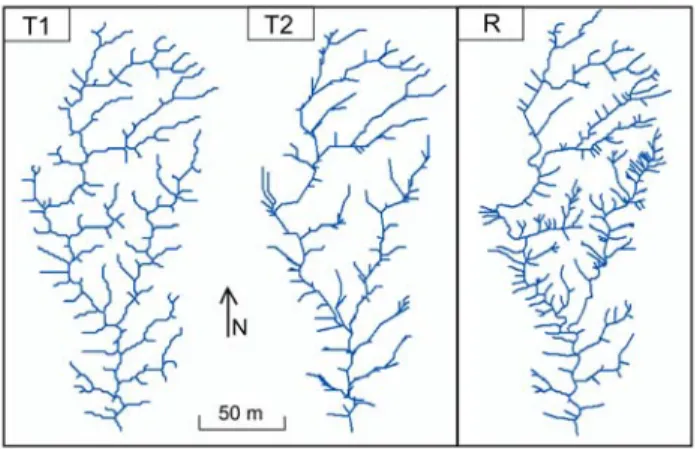
Material 178
The method is applied to compare two extracted networks (T1 179
and T2) to a detailed reference network R (fig. 1) on a test-area of 180
the Draix experimental basins in French Prealps. The study area 181
corresponds to badlands area meaning that terrains are highly 182
dissected. Networks are extracted from a one-meter-resolution 183
airborne LiDAR DTM. The reference is a field-mapped network. 184
185
Figure 1. Comparing extracted networks (T1 and T2) to the ground-truth
186
network (R)
187
The extracted networks result from different extraction 188
method: T1 was extracted using Thommeret et al. (2010) method 189
that combines a morphological index and a drainage algorithm 190
(CI based network); T2 was obtained using the classical D8 191
algorithm (O’Callaghan et Mark, 1984). 192
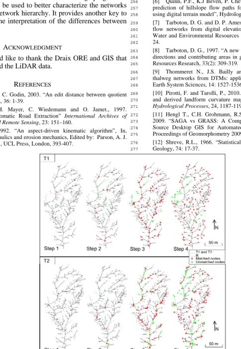
Hierarchical matching results 193
In this particular case study, the distance threshold chosen is 2 194
m, considering that twice the resolution of the base DTM 195
approaches the data’s planimetric noise. The extracted networks 196
have the same number of classes. Every node pairs of both 197
networks are topologically consistent. 198
The matching progression for CI based network and reference 199
is shown figure 2. We can distinguish for each step of the 200
matching the extracted nodes that find a reasonable pair (in red) 201
and those that are not matched (in green). 202
The hierarchical matching process provides step-by-step 203
results. Thus the results are sharper than with the global buffer 204
approach. Step-by-step results for the two extracted networks 205
show different extraction quality (fig. 2). For the CI based 206
network, unmatched nodes are localized in specific areas where 207
the DTM is less accurate. While unmatched nodes of the D8 208
network are dispersed in the space. 209
Global ratios coming from the matching are presented TABLE
210
1. For the CI based network, the matched nodes represent 87% of 211
the total number of nodes. For the D8 network, they represent 212
76%. Thus, the D8 network shows more over-detected nodes 213
than the other network. 214
TABLE I. QUANTITATIVE MATCHING RESULTS
215
Networks Total node
number Pairs
Unmatched nodes
Extracted Reference T1 200 174 26 170 T2 238 181 56 162
DISCUSSION AND CONCLUSION
216
In this paper, we propose an interactive method to 217
quantitatively and automatically compare two networks of a same 218
area. The method aims to help assessing networks extracted from 219
DTM to a reference since more and more elevation data and 220
methods are available to automatically extract thalweg networks. 221
This method relies on hierarchical node matching. It is based 222
on an object-by-object approach which provides more controlled 223
results. The hierarchical approach helps comparing networks 224
represented at different scales. It helps distinguishing extraction 225
artifacts from unmatched nodes resulting from a scale difference 226
between the networks. 227
Results are satisfying and compliant to visual comparison. 228
This method provides results with clear significations that can be 229
directly interpreted: while the buffer method provides global 230
results based on the network overlap, the proposed method 231
supplies more significant and detailed results. Step-by-step 232
matching maps observation helps qualifying the spatial 233
distribution of extraction errors. The matching progression 234
through the steps can be used to better characterize the networks 235
adequacy along the network hierarchy. It provides another key to 236
the assessment and the interpretation of the differences between 237
the networks. 238
ACKNOWLEDGMENT
239
The authors would like to thank the Draix ORE and GIS that 240
acquired and validated the LiDAR data. 241
REFERENCES
242
[1] Ferraro, P. and C. Godin, 2003. “An edit distance between quotient
243
graphs, Algorithmica, 36: 1-39.
244
[2] Heipke, C., H. Mayer, C. Wiedemann and O. Jamet., 1997.
245
“Evaluation of Automatic Road Extraction” International Archives of
246
Photogrammetry and Remote Sensing, 23: 151–160.
247
[3] Lea, N. J., 1992. “An aspect-driven kinematic algorithm”, In,
248
Overland flow: hydraulics and erosion mechanics, Edited by: Parson, A. J.
249
and Abrahams, A. D., UCL Press, London, 393-407.
250
[4] Molloy, I. and T.F. Stepinski, 2007. “Automatic mapping of valley
251
networks on Mars”, Computers & Geosciences, 33:728–738.
252
[5] O’Callaghan, J. and D. Mark, 1984. “The extraction of drainage
253
networks from digital elevation data”, Computer vision, graphics and
254
image processing, 28: 323-344.
255
[6] Quinn, P.F., K.J Beven, P. Chevallier and O. Planchon,, 1991. “The
256
prediction of hillslope flow paths for distributed hydrological modeling
257
using digital terrain model”, Hydrological Processes, 5: 59–79.
258
[7] Tarboton, D. G. and D. P. Ames, 2001. “Advances in the mapping of
259
flow networks from digital elevation data”, In: Proceedings of World
260
Water and Environmental Resources Congress, Orlando, Florida, May
20-261
24.
262
[8] Tarboton, D. G., 1997. “A new method for the determination of flow
263
directions and contributing areas in grid digital elevation models”, Water
264
Resources Research, 33(2): 309-319.
265
[9] Thommeret N., J.S. Bailly and C. Puech, 2010. “Extraction of
266
thalweg networks from DTMs: application to badlands”, Hydrology and
267
Earth System Sciences, 14: 1527-1536.
268
[10] Pirotti, F. and Tarolli, P., 2010. “Suitability of LiDAR point density
269
and derived landform curvature maps for channel network extraction”,
270
Hydrological Processes, 24, 1187-1197.
271
[11] Hengl T., C.H. Grohmann, R.S. Bivand, O. Conrad and A. Lobo,
272
2009. “SAGA vs GRASS: A Comparative Analysis of the Two Open
273
Source Desktop GIS for Automated Analysis of Elevation Data”, In:
274
Proceedings of Geomorphometry 2009, Zurich, August 31- September 3.
275
[12] Shreve, R.L., 1966. “Statistical law of stream number”, Journal of
276
Geology, 74: 17-37.
277
278
Figure 2. Matching progression through the different steps for the two extracted networks (T1 and T2)