Multivariate VaRs for Operational Risk Capital Computation: a Vine Structure Approach

HAL Id: halshs-00587706

https://halshs.archives-ouvertes.fr/halshs-00587706v3

Submitted on 17 Jul 2012

HAL is a multi-disciplinary open access

archive for the deposit and dissemination of sci-entific research documents, whether they are pub-lished or not. The documents may come from teaching and research institutions in France or

L’archive ouverte pluridisciplinaire HAL, est destinée au dépôt et à la diffusion de documents scientifiques de niveau recherche, publiés ou non, émanant des établissements d’enseignement et de recherche français ou étrangers, des laboratoires

Multivariate VaRs for Operational Risk Capital

Computation: a Vine Structure Approach

Dominique Guegan, Bertrand Hassani

To cite this version:

Dominique Guegan, Bertrand Hassani. Multivariate VaRs for Operational Risk Capital Computation: a Vine Structure Approach. 2012. �halshs-00587706v3�

Documents de Travail du

Centre d’Economie de la Sorbonne

Multivariate VaRs for Operational Risk Capital

Computation : a Vine Structure Approach

Dominique G

Bertrand H

2011.17

Multivariate VaRs for Operational Risk Capital Computation: a

Vine Structure Approach

April 25, 2012

Authors

• Dominique Guégan: Université Paris 1 Panthéon-Sorbonne, CES UMR 8174, 106

boule-vard de l’Hopital 75647 Paris Cedex 13, France, phone: +33144078298, e-mail:

dguegan@univ-paris1.fr

• Bertrand K. Hassani: AON and Université Paris 1 Panthéon-Sorbonne CES UMR 8174,

8 Devonshire Square, EC2M 4PM London, United Kingdom, phone: +44 (0)2070860973,

Abstract

The Basel Advanced Measurement Approach requires financial institutions to compute capital requirements on internal data sets. In this paper we introduce a new methodology permitting capital requirements to take into account the embedded dependence structures of operational risks. The loss distributions are provided in a matrix of 56 cells. Constructing a vine architecture, which is a bivariate decomposition of a n-dimensional structure (n > 2), we use this approach to compute multivariate operational risk VaRs. We analyse the results and compare them with classical methodologies based on LDF modelings. Our method is simple to carry out, easy to interpret and complies with the new Basel Committee requirements.

Keywords: Operational risks - Vine Copula - Loss Distribution Function - Nested Structure

1

Introduction

The Basel Committee advanced approaches oblige banks to carry out internal model to evalu-ate the amounts of capital needed to face their risks (BCBS (2004)). In terms of operational

risks, the proposals are still in their infancy, and most banks’ internal strategies are based on traditional models whose assumptions are not always realistic. It may often be observed that

risk managers’ teams use very simple or naive methodologies although the operational risks are intrinsically complex. Indeed, to compute capital allocations, two sets of information

character-ized by different statistical distributions need to be considered. These represent the frequencies and the severities. The presence of correlation and dependencies between severities and/or

fre-quencies have been highlighted by Chernobai et al. (2007). The dependencies must be taken into account in the model design. As the model is more sensitive to the severities than to the

frequencies, the current paper focuses on the dependencies between severities and uses them to derive the overall capital allocation.

In order to comply with Basel II requirements, we propose a novel approach based on recent methodologies to associate a risk measure (e.g. the Value-at-Risk (VaR) (Jorion (2006))) with

the risk profile of a financial institution. Following the Basel Matrix risk classification, we pro-vide an original way to obtain this VaR associated with a medium-sized set of operational risk

categories (> 3) based on the copula methodology. A robust way to measure the dependence between large data sets is to compute their joint distribution function by using copula tools.

Indeed, a copula is a multivariate distribution function linking a large set of data through their standard uniform marginal distributions (Sklar (1959), Nelsen (2006)). In the literature, it has

often been mentioned that the use of copulas is difficult in high dimensions apart from when one uses an elliptic structure (Gaussian or Student) (Di Clemente and Romano (2004)). In

this paper we release these restrictions by considering recent developments on copulas: nested copulas (Morillas (2005), Savu and Trede (2006)) and vine copulas (Aas et al. (2009), Berg and

Aas (2009), Guégan and Maugis (2010), Brechmann et al. (2010) and Dissmann et al. (2011)).

These n-dimensional copulas need to be fed by some marginal distributions. In our case they correspond to the Loss Distribution Function (LDF). As a huge literature for the choice of

severities and frequency distributions (Cruz (2004)) already exists, we will not go any further in details. Thus, in the following we restrict our analysis to the Poisson distribution for the

frequency distribution1 and, for the severity distribution, we consider the empirical, the lognor-mal, the Gumbel and the Generalized Pareto distributions. In our application we show that

the calibration of the severity function plays an important role in the computation of the risks, whatever the method used for the dependence structure. Our results confirm previous facts

already stated in the literature (Gourier et al. (2009), Guégan et al. (2011), etc.) but the new methodology used here permits the detection of specific behavior useful for risk management,

such as the upper tail dependence of the severities.

In a first step, we estimate the severity distributions for each cell of the Basel Matrix (Table 1). In a second step we focus on the choice of the copulas to measure the dependence between these

cells. We use the empirical severity distribution to estimate the parameters of the chosen depen-dence structure, and then we apply this to the LDFs. As soon as we consider higher dimensions,

we face some problems. Traditionally, practitioners use Gaussian or Student’s t copulas. How-ever, as these one are belonging to the elliptic family, they fail to capture asymmetric shocks (by

definition operational risks severity distributions are asymmetric). For example, using a Stu-dent copula with three degrees of freedom2 to capture a dependence between the largest losses,

would also induce a higher correlation between the very low losses. An alternative is found in Archimedean copulas (Joe (1997)) which have attracted particular interest due to their capability

to capture the dependence embedded in different parts of the marginal distributions (right tail, left tail and body). Nevertheless as soon as we want to measure a dependence between more than

two sets, the use of this class of copulas becomes limited as they are generally driven by a single parameter. Therefore traditional estimation methods may fail to capture the dependence

inten-sity. Therefore, a large number of multivariate Archimedean structures have been developed, for instance the fully nested structures, the partially nested copulas and the hierarchical ones.

Nevertheless, all these architectures imply restrictions on the parameters and impose using an Archimedean copula at each node making their use limited in practice, for instance the Archimax

1

Trough our analysis, we tested different other distributions such a the binomial and the negative binomial to model the frequencies and as we have not noticed any sensitivity of the capital charge to these ones, we only used the Poisson distribution.

2

copulas (Capéraà et al. (2000)) which include non-symmetric extreme-value copulas introduced by Gudendorf and Segers (2010). Thus in our application we do not focus on this class of copulas.

To bypass the restrictions imposed by the previous nested strategy, we use an intuitive approach

proposed by Joe (1996), based on a pair-copula decomposition. We limit our analysis to the so-called D-vine (Kurowicka and Cooke (2004)) in which no node in the structure is connected

to more than two edges (Aas et al. (2009)). This approach rewrites the n-density function associated with the n-copula, as a product of conditional marginal and copula densities. We

build iteratively all the conditioning pair densities to get the final one representing the entire dependence structure. The approach is simple, and has no restriction for the choice of functions

and their parameters. Its only limitation is the number of decompositions we have to consider as the number of vines grows exponentially with the dimension of the data sample and thus

requires the user to select a vine from n!₂ possible vines. The optimal strategy to employ is not considered in this paper. We instead refer the interested reader to Antoch and Hanousek (2000),

Bedford and Cooke (2002), Brechmann et al. (2010) and Guégan and Maugis (2011).

To summarize, our strategy not only consists in computing a global capital charge for the finan-cial institution considered, but also in obtaining the standalone contribution of each marginal

distribution to the global capital requirement, which is the most interesting topic for risk man-agers as it enables them to identify the business units which need particular attention. Indeed,

practitioners need to understand which processes engender the largest marginal capital and why.

The paper is organized as follows. In Section 2, we introduce and detail the methodology and the computation of the dependence structure for the Basel Matrix given in Table 1. In Section

3, we present our experimental process and we provide the corresponding capital requirement by lines, columns and for the whole matrix. Section 4 addresses some practical issues. Section

2

A High Dimensional Structure for Operational Risk

In order to leave the elliptical domain to obtain another dependence measure for large data sets, new n-dimensional dependence structures have been proposed in the literature: the nested

struc-tures and the pair-copula strucstruc-tures called vine copulas. Nested and pair-copula architecstruc-tures are based on successive bivariate copula decompositions. Nested copulas based on Archimedean

nodes were originally introduced by Joe (1997), have been studied by Morillas (2005), Savu and Trede (2006) and applied by Aas et al. (2009) and Berg and Aas (2009). They can be divided

in four types: exchangeable nested copulas, fully nested copulas, partially nested copulas and hierarchically nested copulas. The first class imposes very restrictive dependence structures

on the copulas as soon as the number of nodes increases: the m-dimensional marginal distri-butions (m < n) and the generators need to be identical. The three other classes which are

extensions of the first structure are more flexible. Nevertheless they are all constrained by the choice of the copula parameter whose value has to decrease as soon as the level of nodes increases.

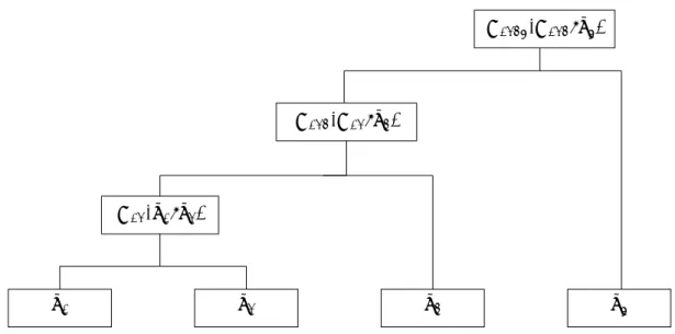
In Figure 1, we illustrate the fully nested copulas in a 4-dimensional case. The initial level is composed of univariate distributions, the second level presents the copula considering

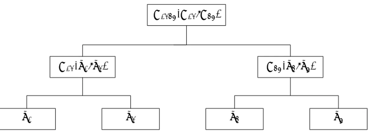
one-dimensional marginals, the third level is built with a copula linking the previous copula and an univariate distribution, and so on. In Figure 2 we illustrate the partially nested copula. The

initial level is composed of distributions representing each Basel category for instance, the second level represents the copulas linking these marginal distributions and the third level corresponds

to the copula linking the two previous ones. The nested architecture which is a very interesting concept in theory is based on assumptions that are too limited to be used in practice.

Pair-copula architectures (Figure 3), suggested by Joe (1996) are more flexible: any class of Pair-copula can be used, and no restriction is required on the parameters. Nevertheless, compared to nested

structures, vine copulas require testing and estimating a large quantity of copulas.

To be more accurate the formal representation of copulas is defined in the following way. Let

X = [X1, X2, ..., Xn] be a vector of random variables, with joint distribution F and marginal

mapping the individual distributions F1, ..., Fnto the joint one F :

F (x) = C(F1(x1), F2(x2), ..., Fn(xn)),

where x = (x₁, x2, ..., xn). we call C a copula.

The Archimedean nested type is the most intuitive way to build n-variate copulas with bivariate

copulas, and consists in composing copulas together, yielding formulas of the following type for

n = 3:

F (x1, x2, x3) = Cθ1,θ2(F (x1), F (x2), F (x3))

= C_θ1(C_θ2(F (x₁), F (x₂)), F (x₃))

where θi, i = 1, 2 is the parameter of the copula. This decomposition can be done several times,

allowing to build copulas of any dimension under specific constraints.

To present the vine copula method, we use here for simplicity its representation through the

density decomposition and not the distribution function as before. Denoting f the density function associated with the distribution F , then the joint n-variate density can be obtained as

a product of conditional densities. For n = 3, we have the following decomposition:

f (x1, x2, x3) = f (x1).f (x2|x1).f (x3|x1, x2),

where

f (x2|x1) = c1,2(F (x1), F (x2)).f (x2),

and c1,2(F (x1), F (x2)) is the density copula associated with the copula C which links the two

marginal distributions F (x₁) and F (x₂). With the same notations we have:

f (x3|x1, x2) = c2,3|1(F (x2|x1), F (x3|x1)).f (x3|x1) = c_2,3|1(F (x2|x1), F (x3|x1)).c1,3(F (x1), F (x3)).f (x3). Then, f (x1, x2, x3) =f (x1).f (x2).f (x3) .c1,2(F (x1), F (x2)).c1,3(F (x1), F (x3)) .c2,3|1(F (x2|x1), F (x3|x1)). (2.1)

That last formula is called vine decomposition. Many other decompositions are possible using different permutations. Details can be found in Berg and Aas (2009), Guégan and Maugis (2010)

and Dissmann et al. (2011).

In the applications below, we focus on these vine copulas and in particular the D-vine whose density f (x₁, ..., xn) may be written as,

n Y k=1 f (xk) n−1 Y j=1 n−j Y i=1

cθ,i,i+j|i+1,...,i+j−1(F (xi|xi+1, ..., xi+j−1), F (xi+j|xi+1, ..., xi+j−1)) (2.2)

where index j identifies the trees, while i runs over the edges in each tree.

To our knowledge such a methodology has never been used to associate a risk measure with

operational risks, and it is new comparing to the works of Di Clemente and Romano (2004) and Gourier et al. (2009) for instance.

C1234(C123, u4)

C123(C12, u3)

C12(u1, u2)

u1 u2 u3 u4

C1234(C12, C34)

C12(u1, u2) C34(u3, u4)

u1 u2 u3 u4

Figure 2: Partially Nested Copula illustration

C123(C12, C23)

C12(u1, u2) C23(u2, u3)

u1 u2 u3

Figure 3: 3-dimensional D-vine illustration: it represents another kind of structure we could have considering a decomposition similar to 2.1, considering the cdfs.

3

Results

The estimation part and the computation of the capital requirement for the Basel matrix is now

3.1 Experimental Process

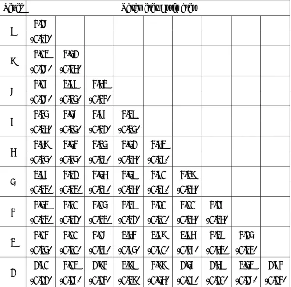
The methodology developed in this paper is applied to the Basel Matrix (BCBS (2001)) given

in Table 1. This Table is composed of 56 cases - 8 business lines ("b") × 7 event types ("e")3. This matrix provides loss amounts corresponding to specific events (fraud, clients’ practice, etc.) which are associated with banks’ business units, and these losses are not considered as time

series. For the whole set of cells, the bank needs to provide a risk measure, and then the capital required to face these risks. In the following, we compute these risks by business units (lines), by

event types (columns) and for the global matrix. The specific loss data set we use for applications has been provided by the French Caisse d’Epargne. We use 99280 data points corresponding to

events which occurred between 2006 and 2008. The descriptive statistics of the data sets are given in Appendix A.

Coming back to the core of our paper, we specify how we are going to work to associate a

risk measure to the whole set of cells provided in Table 1. One of our objectives is to show that it is possible to use multivariate copulas to measure operational risks capital requirements,

beyond the set of elliptical copulas (Gaussian and Student ones). The second objective is to show the influence of the margin and copulas choice on capital computations. We will see that

the choices create large differences in the computation of the capital and, thus the regulator must be informed releasing the rules. We summarize our approach considering the following

three steps:

• In a first step, we estimate the parameters of the severity distributions for the 10 cells

of Table 1 (for which we have enough data sets) chosen among empirical, lognormal and

Gumbel distributions4.

• In a second step, we estimate the dependence structures between these severities using

nested copulas and vine architectures (Brechmann et al. (2010)). We use a pseudo

maxi-3

The business lines are corporate finance, trading & sales, retail banking, commercial banking, payment and settlement, agency services, asset management and retail brokerage. The event types are internal fraud, external fraud, employment practices & workplace safety, clients, products & business practices, damage to physical assets, business disruption & system failures and execution, delivery & process management.

4

Other distributions have been tested but we only provide some results obtained using the Generalized Pareto Distribution in the fifth section

mum likelihood method to estimate the copulas parameters (Mendes et al. (2007), Weiss (2010)) providing the value of the corresponding AIC (Akaike (1974)) in order to

discrimi-nate between different classes of copulas. We select our model following a triple statement: first, we only consider structures which fulfill the theoretical conditions of application;

second between these structures we select the one that presents the lowest AIC; third, we select the structure which provides a conservative capital allocation (BCBS (2010)). We

focus on Gumbel, Clayton and Frank copulas (Nelsen (2006)). We also use the Galambos copula (Galambos (1975)), the Husler-Reiss one (Hüsler and Reiss (1989)) and the Tawn

(Silverman (1986)) one which are interesting because they enable non-linear and tail de-pendences to be taken into account. The multivariate Gaussian copula is also considered

as a benchmark even if regarding the AIC it is always rejected.

• In a third step, after building the LDF which is a convolution of the distribution of the

pre-vious severities with a Poisson distribution (Guégan and Hassani (2009)), whose estimated

parameters are provided in Appendix B, we apply the previous dependence structures on the severities to the LDFs5, and we derive the 99.9% quantile for this n-dimensional LDF

which gives the final capital requirement.

3.2 Estimations

Using the data set introduced in Section two on the period 2006-2008 and denoting Fi, i =

1, ..., 10, the distributions of the severities corresponding to each cell of Table 1, we proceed as follows to estimate the distributions F_i and the dependence structure between the cells.

Using the empirical cdfs F_i, i = 1, ..., 10 as marginal distribution, (Silverman (1986) and Wand

and Jones (1995)), we focus on specific dependence structures between these severity distribu-tions considering different decomposition of the Basel matrix. We first estimate the dependence

between three subsets of cells which are important for the management of the bank because they correspond to specific sectors of activities, and finally we use them to study the whole matrix.

We specify these sets:

5

It should be recalled that we assume that the frequency data sets do not change the structure of dependence obtained from the severities.

BUSINESS BUSINESS LINE S (1) In ternal F rau d (2) External F raud (3) Emplo ymen t Practices & (4) Clien ts, Pro ducts (5) Damage to Ph ysical Assets (6) Business Disruption (7)Execution, Deliv ery UNITS LEVEL 1 W orkplace Safet y & Business Practices & System F ailures & Pro cess Managemen t INVESTMENT BANKING (1) Corp orate Finance (including Municipal/Go v.t Finance & merc han t bankin g) (2) T rading & Sales F1 BANKING (3) Retail Banking F8 F2 F5 F9 (4) Commercial Banking (5) P a ymen t & Settlemen t F10 F3 F6 F7 (6) Agency Service s & Custo dy OTHERS (7) Asset Managemen t (8) Retail Brok erage F4 T able 1: Basel Matrix for op e rational risks: eac h cell represen ts Business line/ev en t typ es classification. Fi , i ∈ [1 , 10] denotes the distribution ass o ciated to eac h cell for whic h data is a v ailable.

1. F2, F5, F8 and F9 which enable modelling event type dependences, considering the "Retail

Banking" business unit;

2. F₃, F₆, F₇ and F₁₀ which enable modelling event type dependences, considering the

"Pay-ment and Settle"Pay-ment" business unit;

3. F1, F2, F3 and F4 which enable modelling business unit dependences, considering the

"Client, Products & Business Practices" event type; and

4. F₁, F₂, F₃, F₄, F₅, F₆, F₇ ,F₈, F₉ and F₁₀, which enable modelling dependencies of the

whole Basel Matrix.

To compare the different methodologies presented previously, we successively link the three first

sets using a multivariate Gaussian copula (denoted A), a partially nested copula (PNC), a fully nested copula (FNC), and finally a vine structure (D), considering Gumbel, Clayton, Frank,

Galambos, Husler-Reiss and Tawn copulas in every case. In order to estimate the successive bi-variate copulas parameters, we carry out pseudo-maximum likelihood methods following Mendes

et al. (2007) and Weiss (2010). In table 3 we provide the estimated parameters for these three sets of 4 cells with the corresponding AIC. We observe that the PNC and FNC methodologies

do not always give results for the dependence structures between the severities because the con-straints on the copula parameters are not verified. For the Gaussian structure, we provide only

the estimated correlation parameter ρ. For the vine approach, we provide the results only for the Gumbel copula because, examining the AIC, it is the best adjustment we obtain for all data sets among the previously mentioned copulas. Comparing adjustments between the multivariate

Gaussian copula and the Gumbel one, with respect to the AIC, the last one provides the best adjustment. We also observe that the vine approach beats the nested one when we are able to

adjust it on a data set: for instance for the subset (F3, F6, F7, F10) (Table 3, second column)

whatever the copula we use.

Then we provide in Tables 4-6 the parameters obtained using a vine strategy modelling the

de-pendence between the 10 severities (whole matrix), using a Gumbel copula (Table 4), a Clayton copula (Table 5) and, a mixture of numerous copula family architectures (Table 6). According

adjustment.

To measure the dependence structure for the whole Basel Matrix (Table 1) reduced to four distri-butions (Table 2) we propose an alternative way. We consider a specific copula architecture using

a Student copula to link these four LDF respectively denoted B1 = F1, B2 = Cθ2(F2, F5, F8, F9), B3 = Cθ3(F3, F6, F7, F10), and B4 = F4. The estimated parameters of the Student copula are

given in Table 7. This structure will be denoted by the term "Overhead" in the following.

Comparing the vine approach and the mixture between the vines and the Student copula, we notice that the log-likelihood retains the vine (Table 6), but according to the AIC (due to the

number of estimated parameters) we should retain the "Overhead" architecture. Nevertheless we continue our exercise with the two methodologies (vine and "Overhead" copula) and we compare

the corresponding capital allocations in the next paragraph.

The choice of the vine decomposition mainly depends on a preliminary analysis of the Basel cells (Table 1). Indeed, the initial structure is given studying the risk supported by Business Units.

In our case, we respectively have on the edge, the Retail Banking, the Trading and Sales, the Retail Brokerage and the Payment and Settlement.

BUSINESS BUSINESS LINES Loss Distributions

UNITS LEVEL 1

INVESTMENT BANKING (2) Trading & Sales B1

BANKING

(3) Retail Banking B2

(5) Payment & Settlement B3

OTHERS (8) Retail Brokerage B4

Table 2: Restricted Basel Matrix used to compute operational risk global capital allocation. B₁,

3.3 Capital Requirements

As soon as the dependence structure between the different cells of the Basel matrix is known,

we use it to provide the corresponding capital requirement. An essential tool to obtain it is the Loss Distribution Function which is computed as a convolution of the distribution characterizing the severities with a Poisson distribution. We recall that the LDF is a mixture of distributions

and details on the methods can be found in Chernobai et al. (2007), Guégan and Hassani (2009) and Guégan et al. (2011) among others.

To obtain the capital requirement associated with the LDF, first based on sets of 4 cells, then

on the whole ten cells four strategies are considered and results are given in Tables 8 - 10.

1. The first strategy consists in associating a VaR measure (and then the corresponding

capital) to each cell, and sum the VaR for the corresponding number of cells. At each time we compute this VaR for the three severity distributions we previously retained (empirical, lognormal and Gumbel). The results of this strategy is provided on the first line of Table

9 for 4-dimensional data sets, and the first line of Table 10 for the whole matrix. We call this approach "univariate" in the Table.

2. To take into account the dependence structures estimated previously on the severities, in the second strategy, we link all the LDFs using a Gumbel copula because it is always the

best one (the lowest AIC). Considering again the three distributions for the severities, we provide in Table 9 (middle line) the corresponding capital requirements for the

4-dimensional data sets, and in Table 10 (bottom line) for the whole matrix using a Student copula.

3. In Table 8, we provide capital values using vines methodology for the 10 marginal distri-butions (following the strategies presented in Tables 4, 5 and 6).

4. In the last line of the Table 9, we provide the capital requirement using a multivariate Gaussian copula, although this adjustment is rejected during the estimation process.

From these results (Tables 8-10) some comments arise:

• We observe that the most conservative value for the capital requirement is obtained when

distri-bution, whatever the strategy used. On the other hand, whatever the dependence structure and the set of severities we consider the largest risk exposure is obtained when we model

the LDF as a convolution of Gumbel and Poisson distributions.

• Whatever the set of severities we consider, the multivariate Gaussian copula applied to

the LDF computed as a convolution of lognormal and Poisson distributions provides the

most conservative results. Note that this strategy is often used by practitioners, but in our case, the Gaussian copula is rejected according to the AIC6.

• The first line of Table 9 exhibits the less conservative results. It corresponds to the classical

strategy used by practitioners (sum of the VaRs). Thus our proposal enables "moderating" the risk-taker behavior of financial agents, taking into account the dependence structure

and providing more conservative values.

Now, in order to compute the global capital value based on the whole Basel Matrix, several strategies may be carried out using the lines and the columns of Table 1:

1. We can compute the VaR for each Basel category and sum the 10 corresponding VaRs. it

is the strategy privileged by practitioners based on a common practice without analysis of the real data sets.7

2. Alternatively, we can use the vine methodology developed previously applying it to the whole structure following the scheme presented in the previous figures, using for instance

an Archimedean copula whose parameter is given in Tables 4, 5 and 6. This is the approach we have privileged in this paper because it lies on a robust computation of the dependence

structure between the cells.

The final capital requirements computed using these two strategies with three different models for the LDFs (empirical (1), lognormal (2) and Gumbel (3)) are given in Table 10. We analyse

the results provided in this one.

6_{We noticed that this conservative result is only due to the fact that we used CDFs to estimate the Gaussian} copulas parameters.

7

We can use the dependence structure previously obtained between the lines and sum the corresponding aggregated VaRs. We can use the same strategy working with the columns. We link vines copulas (for instance, the Gumbel ones) with a Student copula (Table 7).

• The most conservative result is obtained using the Gumbel dependence structure when the

LDF is estimated using a convolution of Poisson and non-parametric distributions: e 76 966 585 (If we do not consider the sum of univariate VaRs as a viable solution)).

• The less conservative result is obtained when we use the "Overhead" structure when each

LDF is computed as a convolution of Poisson and lognormal distribution: e 25 277 957. We observe that our approach taking into account a dependence structure which captures ex-treme events and their frequency provides the most conservative result. It is important to

note that the methodology behind this result is very easy to carry out and could be used by practitioners. We now analyze some points which can be interesting for application purposes.

4

Further developments

In this section, we focus on several important points we have encountered during the previous process applying the vine approach in order to compute the capital requirement associated to

Table 1.

1. Table 9 provides the capital amount for a global set of 4 severities. We can derive by projection the amount corresponding to each severity. This capital is given in Tables 11

- 13. For example, for the fourth column corresponding to "Clients, Products & Business Practices", we can provide the amounts pertaining independently to the "Retail Banking",

the "Trading & Sales", the "Payment & Settlement" and the "Retail Brokerage" business lines. Our approach is interesting because we provide the capital for each cell through the

dependence structure between the cells. This approach is totally different of the approach used by practitioners who directly compute the capital associated to a cell without taking

into account the information given by the other cells.

2. When we estimate dynamically the parameter of the dependence structure we observe

important variations in the values of the Gumbel copula parameter. We illustrate this fact in Table 14. We have computed the parameter of the Gumbel copula linking the LDFs of

the cells F9 and F6. This parameter θ varies with respect to the information set used for its

estimation : the value obtained using the year 2006, is different when we use the year 2007

when we use this last data set. This will have an impact for the computation of capital requirements. Thus, with respect to the information set we use, the capital requirement

appears to be more or less conservative.

3. The impact of the choice of the severity distributions associated with the choice of the dependence structure between these severities is crucial for the computation of the capital

requirement. We illustrate this fact using the distribution which characterizes the cell

F9 corresponding to Business Disruption & System Failure events in the Retail Banking

business unit and the distribution associated to the cell F6 characterizing the same events

in the Payment & Settlement business unit. For the distribution F₉ we use a Gumbel

distribution or a lognormal distribution, for the distribution F6 we use a Generalized

Pareto distribution (GPD) or a lognormal distribution. Table 15 provides the capital

values when we link these two distributions with a Gumbel copula on one hand and with a Clayton copula on another hand. We give the projections of the capital for each cell and

also the global value. Table 15 shows that depending on the way we model the marginal distributions, we have tremendous differences between the VaRs. For example, we would

have a VaR equal to 117 207 402 euros if F9 is modeled with a lognormal distribution and F6 with a GPD distribution versus a VaR equal to 2 037 655 euros if F9 is modeled with

a lognormal distribution and F6 with a Gumbel one. Depending on the way we model the

LDFs, the aggregated VaR may be multiplied by 57.52. The same behavior is observable

when we project the corresponding values on the cells. For example, the multivariate VaR projection on F₉ is e 2 655 055 if F₆ is modeled using a lognormal distribution, and is equal to e 15 405 192 if F6 is modeled using a GPD distribution. The peak for the VaR

observed in that latter case is due to the caption of extreme events through the choice of

the marginal distributions.

4. In Table 15 we observe also that the capital requirements obtained using a Gumbel cop-ula are always bigger than the one obtained with a Clayton one, thus the choice of the

dependence structure has also an important impact on the computation of the capital. Finally, using at the same time, copula and severity distributions which take into account information in the tail provides very accurate results. Indeed, when we model F₆ using a

one. We have to compare the amountse 105 422 356 with e 103 249 260 on the one hand, and e 117 207 402 with e 107 807 238 on the other.

In conclusion, all these results point the importance of the marginal distributions’ and copula’s

modellings to associate a "correct" capital allocation with any risk.

5

Conclusion

This paper proposes a new methodology to compute the capital requirement associated with a

large number of operational risks categories (i.e. n-dimension copulas). We focus on the vine copula architecture which permits the choice of the marginal distributions and of the copulas. We can retain the following main improvements for practitioners:

• Firstly, this methodology enables the use of numerous classes of copulas without being

restricted to the elliptic domain. One can consider copulas which focus on information contained in the tails, where we find the large losses. Recently, we have also shown (Guegan

and Hassani (2011)) that regarding our data sets and the Expected Shortfall as an accurate risk measure, the choice of the Copula structure has a tremendous impact on the capital

requirement. We did not observe this impact when using the VaR.

• Secondly, our approach allows several combinations of marginal distributions to derive

robust adjustments in the statistical sense.

• Thirdly, even working in the high dimension, the procedure is easy to implement and is

not too time consuming8_.

• Finally, our method complies with the new Basel Committee (BCBS (2010)) requirements.

Let us note that the complete Basel matrix could contain more than 250 cells. The open

ques-tion is to be able to work with such a large matrix, whilst limiting the time of computaques-tion. Recent developments based on parallel computing could be an interesting solution in the future

(Brechmann et al. (2010)).

8_{The provided results were obtained with a computer with common capacities i.e. Pentium 4, 3GHz and 1GB} of RAM. We implemented the method with "R-2.11.0". We had no opportunity to parallelized the simulation procedure, therefore each run took between 15 to 30 minutes.

The methodology presented in this paper can be applied to any computation for risk measure-ment and it is not limited to operational risks. The main philosophy of this paper is to provide

a robust and easy tool to associate a measure for a large number of risks, bypassing for the dependence structure the elliptical approach which is not always adapted to the reality.

Structures C2589(F2,F5,F8,F9) AIC C36710(F3,F6,F7,F10) AIC C1234(F1,F2,F3,F4) AIC (A) ρ = 0.665 −14.398 ρ = 0.682 −14.367 ρ = 0.681 −13.918 Gaussian (0.0438) (0.0422) (0.032) (B)  -  - θ = 1.919 −14.211 P N C (0.498) (C)  -  -  -F N C (D) θ = 17.353 −14.592 θ = 3.764 −14.415 θ = 5.345 −14.355 P airCopula (0.642) (0.579) (0.889)

Table 3: Parameters estimation for several dependence structures applied to three sets of four severities. The corresponding standard deviations are provided in brackets. "Gaussian" denotes

a multivariate Gaussian copula structure, "FNC" denotes Fully Nested copulas, "PNC" denotes Partially Nested copulas and "Pair Copula" denotes a Vine structure. A workable nested

struc-ture has been found when the dependence degree was decreasing and the level of nesting increas-ing. For the copulas C₂₅₈₉ and C₃₆₇₁₀ the AIC is better for the Pair Copula structure than for

the Gaussian one. Considering the dependence between F1, F2, F3 and F4, the AIC is better for

the Pair Copula structure than for the Nested one. In all cases, the robust dependence structure

Level Parameter Estimates 9 3.17 (0.31) 8 3.02 3.41 (0.17) (0.25) 7 3.06 2.99 3.52 (0.17) (0.24) (0.33) 6 3.34 3.47 3.66 3.29 (0.25) (0.24) (0.31) (0.24) 5 3.58 3.43 3.24 3.41 3.52 (0.34) (0.34) (0.27) (0.35) (0.26) 4 2.96 3.21 3.45 3.49 3.60 3.28 (0.22) (0.22) (0.29) (0.25) (0.29) (0.25) 3 3.42 3.30 3.04 3.29 3.10 3.00 3.16 (0.22) (0.21) (0.22) (0.31) (0.20) (0.25) (0.25) 2 3.03 3.00 3.07 2.53 2.78 2.95 3.27 3.14 (0.24) (0.20) (0.26) (0.64) (0.60) (0.36) (0.52) (0.23) 1 1.60 3.02 1.83 2.89 3.88 1.46 1.59 2.42 1.63 (0.11) (0.16) (0.13) (0.28) (0.45) (0.09) (0.10) (0.17) (0.13)

Table 4: This table presents estimates at each node of a Vine built with Gumbel copulas

regard-ing the ten marginal distributions: F1, ..., F10. The standard deviations are provided in brackets.

Level Parameter Estimates 9 1.44 (0.14) 8 1.32 1.24 (0.15) (0.18) 7 1.14 1.14 1.25 (0.17) (0.17) (0.18) 6 1.38 1.06 1.05 1.11 (0.26) (0.17) (0.19) (0.17) 5 1.10 1.16 1.02 1.12 1.29 (0.15) (0.15) (0.15) (0.17) (0.16) 4 1.32 1.23 1.32 0.99 1.33 1.15 (0.14) (0.11) (0.16) (0.12) (0.14) (0.17) 3 1.20 1.31 1.02 1.28 1.05 1.15 1.38 (0.20) (0.18) (0.14) (0.25) (0.21) (0.18) (0.25) 2 0.95 1.02 1.30 1.17 1.15 1.02 1.44 1.22 (0.23) (0.15) (0.17) (0.21) (0.15) (0.13) (0.21) (0.16) 1 0.36 2.89 0.80 1.27 1.78 0.26 0.47 1.14 0.42 (0.11) (0.21) (0.12) (0.22) (0.40) (0.10) (0.12) (0.15) (0.12)

Table 5: This table presents estimates at each node of a Vine built with Clayton copulas

regard-ing the ten marginal distributions: F1, ..., F10. The standard deviations are provided in brackets.

Level Parameter Estimates 9 Frank 12.95 (1.24) 8 Frank Galambos 13.43 2.38 (1.32) (0.24) 7

Husler-Reiss Gumbel Frank 3.62 3.75 13.49 (0.32) (0.30) (1.32)

6

Galambos Frank Gumbel Frank 2.99 13.84 3.45 12.83 (0.38) (1.29) (0.33) (1.38)

5

Husler-Reiss Galambos Frank Gumbel Frank 3.07 2.70 13.35 3.46 12.94 (0.27) (0.33) (1.21) (0.32) (1.15)

4

Frank Gumbel Galambos Gumbel Frank Clayton 13.47 3.25 2.58 3.33 14.06 1.19 (1.13) (0.20) (0.22) (0.23) (1.43) (0.23)

3

Gumbel Galambos Husler-Reiss Galambos Gumbel Frank Clayton

3.44 2.96 3.06 2.89 3.40 13.81 1.12

(0.26) (0.29) (0.26) (0.32) (0.29) (1.24) (0.19)

2

Galambos Frank Galambos Gumbel Gumbel Frank Husler-Reiss Clayton

2.16 13.96 2.83 3.55 3.65 13.67 3.49 0.72

(0.32) (1.51) (0.24) (0.32) (0.36) (1.33) (0.26) (0.30)

1

Franck Gumbel Clayton Galambos Husler-Reiss Tawn Gumbel Clayton Frank

3.24 3.02 0.80 2.19 3.61 3.85 1.59 1.14 3.58

(0.49) (0.16) (0.12) (0.28) (0.41) (0.09) (0.10) (0.15) (0.53)

Table 6: This table presents estimates at each node of a Vine built with 6 different copulas

regarding the ten marginal distributions: F1, ..., F10. The standard deviations are provided in

Structures CB1,B2,B3,B4 AIC

Student Copula ρ = (0.02857775, 0.83355628, 0.08367086, 46.83165

, 0.01551715, −0.17840772, 0.03647245)

(0.002, 0.1, 0.07, 0.001, 0.05, 0.001)

Table 7: This table provides the Student copula parameters obtained modeling the dependence structure between all business lines. The corresponding standard deviations are provided in

Approach LDF CGlobal(F1,...,F10) Univariate 1 77 018 239 2 74 360 305 3 48 871 039 Gumbel Copula 1 76 966 585 2 73 495 616 3 48 851 507 Frank Copula 1 69 647 495 2 62 218 480 3 48 294 940 Clayton Copula 1 64 659 214 2 57 330 189 3 47 887 238

Table 8: This table provides the capital allocation for the whole data set, considering three classes

of severities (1 denotes the non parametric approach of the LDF, 2 the lognormal approach and 3 the Gumbel one.) and three classes of dependence, a Gumbel structure, a Frank one and a

Approach LDF C1234(LDF1,LDF2,LDF3,LDF4) C2589(LDF2,LDF5,LDF8,LDF9) C36710(LDF3,LDF6,LDF7,LDF10) Univariate 1 29 400 454 39 287 139 28 449 066 2 22 794 418 24 118 977 34 614 408 3 8 968 115 25 755 128 15 719 280 Gumbel 1 30 646 550 41 456 461 33 252 197 2 35 474 559 56 176 428 60 970 007 3 21 778 827 25 798 375 15 762 291 Gaussian 1 31 257 604 43 621 089 37 158 832 2 40 651 444 75 785 269 68 385 483 3 21 381 957 25 972 225 15 881 606

Table 9: This table provides the capital allocation (a 99.9% VaR) for 4-dimensional data sets, considering three classes of severities (1 denotes the non parametric approach of the LDF, 2

the lognormal approach and 3 the Gumbel one.) and three classes of dependence. Univariate corresponds to the VaRs sum of each LDF, Gumbel corresponds to the Gumbel copula and

Approach LDF CGlobal(B1,B2,B3,B4) Univariate 1 77 018 239 2 74 360 305 3 48 871 039 Student Copula 1 41 853 691 2 25 277 957 3 33 980 264

Table 10: This table provides the capital allocation for the whole data set, considering three

classes of severities (1 denotes the non parametric approach of the LDF, 2 the lognormal approach and 3 the Gumbel one.) and two classes of dependence. Univariate corresponds to the VaRs

sum of each LDF, Student corresponds to the Student copula used considering that B2 and B3

are themselves vine structure and B1 and B4 univariate LDFs (Table 2).

Approach LDF LDF1 LDF2 LDF3 LDF4 Univariate 1 278 423 19 650 986 467 434 9 003 611 2 254 095 6 240 984 926 513 15 372 825 3 232 591 13 590 317 212 451 7 164 041 Gumbel Copula 1 280 423 20 556 466 524 137 9 285 523 2 377 479 9 957 836 6 283 207 18 856 037 3 714 190 13 602 350 260 749 7 201 537 Gaussian Copula 1 287 179 21 110 804 603 161 9 256 460 2 609 358 9 862 421 3 098 797 27 080 869 3 237 529 13 632 720 213 645 7 298 063

Table 11: This table provides the VaRs associated with each LDF of the set LDF₁, LDF₂,

LDF3 and LDF4 when we decompose the dependence structure of the 4-dimensional set C1234,

considering three classes of severities (1 denotes the non parametric approach of the LDF, 2 the

Approach LDF LDF2 LDF5 LDF8 LDF9 Univariate 1 19 650 986 3 182 731 14 212 411 2 241 011 2 6 240 984 2 151 627 11 676 534 4 049 831 3 13 599 313 2 478 087 8 599 313 1 087 410 Gumbel Copula 1 20 578 056 3 300 471 15 191 828 2 386 106 2 10 732 933 2 310 337 29 525 155 13 608 000 3 13 617 419 2 486 453 8 603 916 10 905 587 Gaussian Copula 1 22 269 192 3 301 720 15 482 009 2 568 168 2 14 264 778 4 157 787 30 072 894 27 259 810 3 13 692 945 2 492 189 8 679 579 1 107 512

Table 12: This table provides the VaRs associated with each LDF of the set LDF₂, LDF₅,

LDF8 and LDF9 when we decompose the dependence structure of the 4-dimensional set C2589,

considering three classes of severities (1 denotes the non parametric approach of the LDF, 2 the

Approach LDF LDF3 LDF6 LDF7 LDF10 Univariate 1 467 435 2 739 085 1 295 941 23 946 606 2 926 513 306 553 2 425 710 30 955 632 3 212 451 772 003 829 360 13 905 464 Gumbel Copula 1 628 263 3 220 812 1 473 900 27 929 223 2 4 191 332 832 333 11 559 821 44 386 520 3 213 844 775 924 831 552 13 940 970 Gaussian Copula 1 584 053 3 572 152 1 394 149 31 608 479 2 7 105 044 1 257 046 12 247 696 47 775 697 3 216 849 789 476 831 840 14 053 440

Table 13: This table provides the VaRs associated with each LDF of the set LDF₃, LDF₆,

LDF7and LDF10when we decompose the dependence structure of the 4-dimensional set C36710,

considering three classes of severities (1 denotes the non parametric approach of the LDF, 2 the

lognormal approach and 3 the Gumbel one.).

Year θ θ

2006 4.9202 (0.94)

10.6610 (0.88) 2007 3.7206 (0.75)

2008 5.8490 (0.51)

Table 14: Parameter estimation of Gumbel copulas estimated on F9 and F6 for each year 2006,

2007 and 2008 (second column). These parameters are compared to a Gumbel copula parameter

estimated on the whole chronicle (third column). The corresponding standard deviation are provided in brackets.

Model Gumbel Copula Clayton Copula

LDF9 LDF6 Sum LDF9 LDF6 Sum

Gumbel-GPD 2 322 782 103 099 574 105 422 356 1 154 681 102 094 579 103 249 260

Gumbel-lognormal 1 471 343 566 312 2 037 655 1 455 693 649 164 2 104 857

lognormal-GPD 15 405 192 101 802 210 117 207 402 5 631 004 102 176 234 107 807 238

Table 15: For the LDF corresponding to F9 and F6we provide the VaRs computed from Gumbel

and Clayton copulas for the year 2006. They are given respectively for three classes of severities.

For instance, "Gumbel-GPD" means that we have chosen a Gumbel distribution to model F9

and a mix of a lognormal and a GPD to model F₆.

A

Appendix: Distributions statistics

Next table provides the four first moments of the empirical severities used in this paper.

Distributions Mean Variance Skewness Kurtosis

F1 195.37 292732.86 7.31 71.69 F2 1522.83 372183311.54 27.57 910.13 F3 175.42 3804557.63 30.03 956.75 F4 1805.81 93274002.03 18.74 457.58 F5 1824.95 189175093.33 17.79 354.00 F6 1200.08 438224165.80 23.69 563.48 F7 800.14 24268504.39 10.88 139.39 F8 1779 1602373386 19.27 435.88 F9 1824.95 189175093.3 17.79 354.00 F10 12104 519962084.2 108.03 11806.23

Table 16: Statistics of the data sets used. The distributions are right skewed and present large

B

Appendix: LDF Parameters

This appendix provides LDF’s parameters estimations regarding considered models.

Distributions Poisson lognormal Gumbel

F1 λ = 1094 µ = 4.03 σ = 1.47 u = 149.88 β = 72.98 F2 λ = 8448 µ = 4.25 σ = 1.97 u = 1381.07 β = 210.43 F3 λ = 1114 µ = 2.80 σ = 2.23 u = 150.02 β = 40.65 F4 λ = 3811 µ = 5.72 σ = 1.99 u = 1443.89 β = 585.89 F5 λ = 521 µ = 4.87 σ = 2.19 u = 848.76 β = 471.77 F6 λ = 575 µ = 4.03 σ = 1.71 u = 1101.79 β = 143.73 F7 λ = 937 µ = 3.72 σ = 2.27 u = 721.71 β = 135.75 F8 λ = 1178 µ = 5.42 σ = 2.14 u = 4010.25 β = 833.45 F9 λ = 8748 µ = 4.87 σ = 2.19 u = 1612.31 β = 370.63 F10 λ = 12103 µ = 5.49 σ = 2.00 u = 861.38 β = 437.14

Table 17: This table provides the parameters estimation for each LDF for the year 2008, assuming a Poisson distribution to model the frequencies, and either a lognormal or a Gumbel distribution

to model the severities.

Distributions Poisson-Gumbel LDF9 λ = 658 u = 191.5378, β = 938.9768 (s.e. 36.70), (s.e. 35.64) Distributions Poisson-GPD LDF6 λ = 1292 µ = 5.70, σ = 1.10 u = 1645.07, β = 932.854, ξ = 0.767

Table 18: This table provides two LDFs’ parameters, LDF₆ and LDF₉, for the year 2006,

assuming a Poisson distribution to model the frequencies and either a Gumbel or a mix of a lognormal and a GPD to model the severities.

C

Appendix: Value-at-Risk

Recall that given a confidence level α ∈ [0, 1], the VaR associated to a random variable X is given by the smallest number x such that the probability that X exceeds x is not larger than

(1 − α).

References

Aas, K., Czado, C., Frigessi, A. and Bakken, H. (2009), ‘Pair copula constructions of multiple dependence.’, Insur. Math. Econ. 44, 182–198.

Akaike, H. (1974), ‘A new look at the statistical model identification.’, IEEE Transactions on

Automatic Control 19, 716–723.

Antoch, J. and Hanousek, J. (2000), ‘Model selection and simplification using lattices.’,

CERGE-EI Working Paper, Charles University in Prague, Czech Republic .

BCBS (2001), ‘Working paper on the regulatory treatment of operational risk’, Basel Committee

on Banking Supervision, Basel, Switzerland .

BCBS (2004), ‘Basel 2: International convergence of capital measurement and capital standards:

a revised framework’, Basel Committee on Banking Supervision, Basel, Switzerland .

BCBS (2010), ‘Basel committee: Operational risk - supervisory guidelines for the advanced measurement approaches - consultative document’, Basel Committee on Banking Supervision,

Basel, Switzerland .

Bedford, T. and Cooke, R. (2002), ‘Vines: A new graphical model for dependent random vari-ables.’, The Annals of Statistics 30(4), 1031–1068.

Berg, D. and Aas, K. (2009), ‘Models for construction of multivariate dependence - a comparison

study’, The European Journal of Finance 15, 639–659.

Brechmann, E., Czado, C. and Aas, K. (2010), ‘Truncated regular vines in high dimensions with applications to financial data.’, Submitted preprint. .

Capéraà, P., Fougères, A. and Genest, C. (2000), ‘Bivariate distributions with given extreme value attractor.’, Journal of Multivariate Analysis 72, 30–49.

Chernobai, A., Rachev, S. T. and Fabozzi, F. J. (2007), Operational Risk: A Guide to Basel II

Capital Requirements, Models, and Analysis, John Wiley & Sons.

Di Clemente, A. and Romano, C. (2004), ‘A copula-extreme value theory approach for modeling operational risk’, Operational Risk Modelling and Analysis pp. 189–208.

Dissmann, J., Brechmann, E., Czado, C. and Kurowicka, D. (2011), ‘Selecting and estimating

regular vine copulae and application to financial returns.’, Submitted preprint. .

Galambos, J. (1975), ‘Order statistics of samples from multivariate distributions.’, Amer. Statist.

Assoc. 10, 674–680.

Gourier, E., Farkas, W. and Abbate, D. (2009), ‘Operational risk quantification using extreme

value theory and copulas: from theory to practice.’, The Journal of Operational Risk 4.

Gudendorf, G. and Segers, J. (2010), Extreme-value copulas. In: Proceedings of the Workshop

on Copula Theory and Its Applications held in Warsaw (editor: P. Jaworski), Springer Media,

New York.

Guegan, D. and Hassani, B. (2011), ‘Operational risk: A basel ii++ step before basel iii.’,

Working Paper, University Paris 1 .

Guégan, D. and Hassani, B. K. (2009), ‘A modified panjer algorithm for operational risk capital calculations’, The Journal of Operational Risk 4, 53 – 72.

Guégan, D., Hassani, B. K. and Naud, C. (2011), ‘An efficient threshold choice for the

compu-tation of operational risk capital’, The Journal of Operational Risk 6, 3 – 19.

Guégan, D. and Maugis, P.-A. (2010), ‘New prospects on vines.’, Insurance Markets and

Com-panies: Analyses and Actuarial Computations 1, 4–11.

Guégan, D. and Maugis, P.-A. (2011), ‘An econometric study for vine copulas.’, to appear in:

International Journal of Economics and Finance .

Hüsler, J. and Reiss, R. (1989), ‘Maxima of normal random vectors: Between independence and complete dependence.’, Statistics & Probability Letters 7, 283–286.

Joe, H. (1996), ‘Families of m-variate distributions with given margins and m(m−1)₂ bivariate

de-pendence parameters.’, Distributions with Fixed Marginals and Related Topics, Lecture

Joe, H. (1997), Multivariate models and dependence concepts., Monographs on Statistics and Applied Probability, Chapman and Hall, London.

Jorion, P. (2006), Value at Risk: The New Benchmark for Managing Financial Risk,

McGraw-Hill Paris.

Kurowicka, D. and Cooke, R. M. (2004), ‘Distribution - free continuous bayesian belief nets.’,

In Fourth International Conference on Mathematical Methods in Reliability Methodology and Practice, Santa Fe, New Mexico. .

Mendes, B., de Melo, E. and Nelsen, R. (2007), ‘Robust fits for copula models’, Comm. in Stat.:

Sim. Comp 36, 997–1017.

Morillas, P. (2005), ‘A method to obtain new copulas from a given one.’, Metrika 61, 169–184.

Nelsen, R. (2006), An Introduction to Copulas., Springer Series in Statistics, Berlin, Germany.

Savu, C. and Trede, M. (2006), ‘Hierarchical archimedean copulas.’, Working Paper, University

of Münster, Germany .

Silverman, B. W. (1986), Density Estimation for statistics and data analysis, Chapman and

Hall/CRC.

Sklar, A. (1959), ‘Fonctions de répartition à n dimensions et leurs marges’, Publ. Inst. Stat.

8, 229–231.

Wand, M. P. and Jones, M. C. (1995), Kernel Smoothing, Chapman and Hall/CRC.

Weiss, G. (2010), ‘Copula parameter estimation - numerical considerations and implications for