Calculation of Higher-Order Fluxes in Symmetric Cores—II: Implementation

HAL Id: cea-02387104

https://hal-cea.archives-ouvertes.fr/cea-02387104

HAL is a multi-disciplinary open access archive for the deposit and dissemination of sci-entific research documents, whether they are pub-lished or not. The documents may come from teaching and research institutions in France or abroad, or from public or private research centers.

L’archive ouverte pluridisciplinaire HAL, est destinée au dépôt et à la diffusion de documents scientifiques de niveau recherche, publiés ou non, émanant des établissements d’enseignement et de recherche français ou étrangers, des laboratoires publics ou privés.

Cores-II: Implementation

Maxence Maillot, Jean Tommasi, G. Rimpault

To cite this version:

Maxence Maillot, Jean Tommasi, G. Rimpault. Calculation of Higher-Order Fluxes in Symmetric Cores-II: Implementation. Nuclear Science and Engineering, Academic Press, 2017, 184 (2), pp.190-207. �10.13182/NSE16-5�. �cea-02387104�

Calculation of Higher-Order Fluxes in Symmetric

Cores—II: Implementation

Maxence Maillot,* Jean Tommasi, and Gérald Rimpault

CEA, DEN, SPRC, CEA-Cadarache, 13108 Saint Paul lez Durance, France Received January 8, 2016

Accepted for Publication June 5, 2016 http://dx.doi.org/10.13182/NSE16-5

Abstract — In neutron chain systems with material symmetries, various k-eigenvalues of the neutron balance equation beyond the dominant one may be degenerated. As shown in a companion paper, the power iteration method can be used to compute higher eigenfunctions in symmetric systems, provided that the global problem is partitioned into symmetry class–related lower-sized problems with appropriate boundary conditions. Those boundary conditions have been implemented in the diffusion solver of the ERANOS code system in rectangular geometry and within the framework of a discontinuous Galerkin spatial approximation of the multigroup discrete ordinates transport equation in the SNATCH solver. Numerical results in homogeneous geometry are provided for verification purposes, as well as the first eigenfunctions of the Takeda benchmarks. Finally, the transport effect on the first flux harmonics for an industrial-sized reactor ZPPR-18 is discussed.

Keywords — Flux eigenmodes, symmetry, degeneracy.

Note — Some figures may be in color only in the electronic version.

I. PRACTICAL IMPLEMENTATION

I.A. Overview of Some Matters Using Traditional

Filtering Techniques

For its conceptual simplicity, and as the dominant

k-eigenvalue is simple, the power iteration method has

been widely used to access the fundamental eigenpair (k0, ⌽0). This method has been extended to access high-order eigenfunctions and eigenvalues, taking advantage of the F-orthogonality properties of eigenfunctions associ-ated with distinct eigenvalues.1,2_{This is called the filtering}

technique. However, some differences between the fun-damental mode (always positive) and the harmonics may lead usual iterative solvers to fail.

First, as the higher harmonics have nodal lines or surfaces and change sign when crossing them, it may prove difficult, if not unachievable, to reach tight relative pointwise convergence criteria in their vicinity. However,

with the absolute value of the flux at such points being small, a degraded relative convergence will have negligi-ble impact on any integral value (multiplication factor, integrated reaction rates). Then, the idea is to test for tight relative convergence only in nodes where the flux is not close to 0. To define the condition to be met before testing convergence, the average of the absolute-value flux is computed. Then, a threshold is chosen by the user (typi-cally 5% of this average absolute value). For nodes where the absolute flux is below this threshold, convergence is not tested. Such development allows the code to reach high-order harmonics.

Second, for symmetric geometries (or invariant under discrete rotations), which are the main assumption of this work, the first harmonic may be odd over the system, so that its integral is null. In the normalization step of the power iteration method, some solvers use the algebraic sum as a mathematical norm. In case of antisymmetric functions, such sum may be null, whereas the vector is not null: In other words the algebraic sum is not a norm. This mistake leads to awkward behavior in the iterative

process. The solution consists of computing a true norm in the solver (L1_norm㛳x㛳1⫽ 兺

ⱍ

i

ⱍ

兹

infinity norm㛳x㛳_⬁⫽ max

ⱍ

ⱍ

A last word is to be said about initialization of the power iteration in symmetric cases. The default shape is a vector with uniform distribution (e.g., all compo-nents equal to 1). Such vector shares the same symme-tries as the material distribution and the fundamental mode. When the first harmonic is computed in the whole reactor (i.e., without using the reduced-size problems), the filtering method may lead to the first harmonic of this symmetry class. Indeed, at each iter-ation, the current vector keeps sharing the same sym-metry properties as the fundamental mode. After removing its contribution, the new vector is still sym-metric and may converge toward the first symsym-metric harmonic, unless numerical discrepancies such as round-off errors eventually break the symmetry. How-ever, the real first harmonic may be of another symme-try class than the fundamental. In this case, the initial guess for the eigenvector (by default, a homogeneous shape) has no projection over the first harmonic, although this is a requirement for the power iteration method to work properly. This would result, for exam-ple, in a bad prediction for the eigenvalue separation (EVS) of the system when the reduced-size problems are not used. This point is illustrated below in an industrial-sized case (ZPPR-18 in Sec. IV).

I.B. Invariance Under Symmetry Operators

In this section, the geometry is assumed to be Cartesian. This is not a requirement since the theory is verified in other frames. The aim is indeed to take advantage of the current development of transport equation solvers. For instance, in case of mirror symmetries, the classical reflection boundary condition allows finding eigenfunctions symmetric with respect to a mirror symmetry plane. Such capability is gen-erally offered both in deterministic or Monte Carlo (specular mirror boundary condition) codes. The search for eigenfunc-tions antisymmetric with respect to a mirror symmetry plane depends on the solver used:

1. In the diffusion approximation, where the angular variable disappears, such antisymmetric functions can be computed using a zero flux boundary condition. This capa-bility is offered by the finite difference solver in rectangular geometry available in the ERANOS code system.3_{The only}

way for the zero flux boundary conditions to lead to a symmetric eigenfunction is that the current is also null on the interface. In such cases, this function could be either sym-metric or antisymsym-metric. In practice, such behavior was not

observed during the work, and the zero flux boundary con-dition is well adapted to our purposes. Moreover, in analyt-ical cases (e.g., if Laplacian eigenfunctions are sinusoidal functions), it is even impossible.

2. Transport solvers do not provide equivalent zero flux boundary conditions, especially because the angular variable has to be taken into account. To our knowledge, the condition for the antisymmetric problems has been used only occasionally, e.g., it is the antireflective boundary condition.4–6_{During the implementation work of such odd}

reflection, we can gain benefit from the developments made for the reflective boundary conditions. In fact, only the eigenvalueε of the symmetry operators changes from ⫹1 to ⫺1. It is the one change to be done to simulate these innovative boundary conditions. Of course, such a change may cause a few problems in Monte Carlo solvers, when negative weights for the neutron are not allowed. On the contrary, deterministic codes often authorize negative val-ues for the flux, provided that the possible implemented fixups are disabled.

For mirror symmetries, if ε (the eigenvalue of the symmetry operator) equals 1 (symmetric function) or⫺1 (antisymmetric function), the boundary condition on the interface is given byEq. (1):

S⌽(␻) ⫽ ⌽关S⫺1(␻)兴⫽ ⌽

关

(

)

(

)

兴

关

兴

I.C. Invariance Under Discrete Rotations

In this section, we consider only rotation of order 3 (i.e., of angle 2␲/3) and of order 4 (i.e., of angle ␲/2). The first one concerns hexagonal geometries and is well adapted to the Advanced Sodium Technological Reactor for Industrial Demonstration (ASTRID) low-void-effect core design.7_{Moreover, some work was already done to}

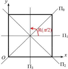
solve the transport equation in a one-third core, while equivalent capabilities are not offered for a six-order rota-tion case (i.e., of angle␲/3). The ␲/2 rotation case was done mainly for verification purposes. Indeed, if a system is invariant for such a rotation, it is probably because this system is also invariant under vertical mirror symmetry planes ⌸0,⌸1separated by an angle ␲/4 (seeFig. 1). In such a case, the previous symmetry boundary conditions can be used over a sector, thus avoiding the treatment of rotation classes. Nevertheless, such development was done in the Cartesian case to verify the filtering technique and the coupled problem. It allows resolution of pure ␲/2-rotation-invariant cases. Deterministic codes used in

this work are the finite difference diffusion solver of the ERANOS code system [the new order-4 rotation bound-ary conditions were implemented only in a development version in two-dimensional (2-D) Cartesian geometries for verification purposes]. The transport code was the discrete ordinates solver SNATCH of the PARIS platform8,9_:

␲/2 rotation in Cartesian geometries and 2␲/3 rotation in hexagonal geometries.

In the ERANOS code system, periodic boundary con-ditions are available for the finite difference diffusion solver. It may be called the translation boundary condi-tion. Invariance under a rotation operator is a kind of periodic condition. Nevertheless, instead of linking the opposite faces of the geometry, now the right side must be connected to the left side of the sector core. This involves specific computations for the matrix expression of the diffusion equation (production and disappearing opera-tors). On the interface, the gradient terms are computed using the flux of both sides to be connected. Finally, calculation is performed on a sector. R-invariant functions are obtained by computing in the sector for functions u such as u(␻⫺) ⫽ u(␻⫹) with, in diffusion theory, ␻ ⫽ ( r¡, E) (no angular dependence). For R-antisymmetric functions, the edges are linked instead by u(␻⫺) ⫽ ⫺u(␻⫹_{). For the coupled problem, we search} simulta-neously for two solutions u and v on the sector linked by Eq. (2):

兵

v(␻⫺) ⫽ u(␻⫹) . (2)

Then, we build the solutions U and V on the whole geometry from the sector solutions u and v [see Eq. (3) below and Sec. IV.B of the companion paper10_]:

兵

V⫽ v ⫺ Ru ⫺ R2_v⫹ R3_{u . (3)}

The coupled problem therefore needs to handle two vectors. On the sector, each vector is independent from the other one, so that the inner iterative process may be done simultaneously (parallelism). Once the inner process is done, both computations may exchange their boundary conditions. The diffusion solver in the ERANOS code system was modified only for the order-4 rotation invariance.

For the transport solver, based on the discrete ordi-nates method and discontinuous Galerkin (DG) schemes (SNATCH solver), both rotations (of angles ␲/2 and 2␲/3) were developed. The idea here is to connect the outgoing flux toward one face of the sector to the ingoing flux toward the other face. Such periodic conditions are already available for the hexagonal solver [where compu-tation can be done over one-third of the core in the case of invariance such as the CFV (French acronym for low sodium void effect core design concept)]. It allows finding the R-invariant eigenfunctions. Then, the cou-pled problem is done in the same way as was previously done for the Cartesian geometry. In the case of order-3 rotation invariance, the boundary condition connecting is Eq. (4):

兵

Finally,Eq. (5)builds the solutions U and V on the whole geometry from the sector solutions u and v:

兵

As one can notice, such innovative boundary condi-tions use methods or tools that are very common in deter-ministic solvers. With only a few changes, the usual solvers are now able to compute a larger number of flux harmonics by sorting them according to their symmetry classes.

Fig. 1. Cross section of a prismatic square homogeneous system with trace of the mirror symmetry planes (⌸0

through⌸3), with␲/4 clockwise angle between one and

the next. R ⫽ S0S1 is the counterclockwise rotation of

II. VERIFICATION STRATEGY FOR THE INNOVATIVE

BOUNDARY CONDITIONS

In this section, we propose a verification of the new boundary conditions that allow the computation of high-order flux harmonics. The first example involves monoenergetic diffusion over a 2-D homogeneous fuel square. Looking for k-eigenfunctions of the diffusion equation is then equivalent to searching eigenfunctions of the Laplacian operator. Such a case provides verifi-cation for the diffusion solver (ERANOS). The eigen-value problem may be solved using rotation class par-tition or symmetry class parpar-tition. The second example involves simple homogeneous geometries treated in the monoenergetic case with the transport solver SNATCH. Extrapolation distance theory is used to match analyt-ical cases (the eigenfunction of the Laplacian operator). The size of the geometries is also progressively increased to reduce the transport effect when comput-ing high-order flux harmonics. This transport solver verification is done for a square and a regular hexagon. Verification is done in two dimensions for simplicity. Material data are given in Table I.

The diffusion equation is given byEq. (6):

⌬⌽ ⫹ ␯

兺

兺

Scattering is assumed isotropic. The eigenvalue k divides only the fission production term. The material used has an infinite multiplicative factor k_⬁⫽ ␯ 兺fis

兺abs

of 1.5, a diffusion coefficient D ⫽ 1

3兺tot

⬇ 1 cm, and a migration area

M2⫽ D 兺abs

⬇ 200 cm2_.

II.A. The Homogeneous Square in the

Diffusion Approximation

We consider here the homogeneous square (x, y)僆 关0; a兴2_{, with Dirichlet boundary conditions on the faces} (see Fig. 1). Eigenfunctions and eigenvalues for ⌬S ⫹ ␹2_S⫽ 0 are then given by _{Eq. (7) (m and n being} non-negative integers and the origin O being taken at a vertex of the square and the coordinate axes along the two orthogonal sides originating from this vertex):

Smn(x, y)⫽ sin

(

)

(

)

The Smn forms an orthogonal system: 兰SmnSm⬘n⬘dxdydz ⫽ 0 for (m, n) ⫽ (m⬘, n⬘). The eigenvalue remains invariant when permuting indices. Unless there is more than one representation of the eigenvalue by the quadratic form (m2 _{⫹ n}2_{), the eigenvalue is simple if indices are} equal, of degeneracy order 2 if indices are different. Let R be the order-4 rotation, S0 the mirror symmetry with respect to the main diagonal x ⫽ y, S1 the mirror symmetry with respect to the x-axis, S2 the mirror symmetry with respect to the off-diagonal, and finally

S3 the mirror symmetry with respect to the y-axis (see Fig. 1), so that the symmetry group used here is

C4v ⫽ 兵I, R, R2, R3, S0, S1, S2, S3其.

We use this square geometry to validate the testing of the innovative symmetry and rotation boundary condi-tions described in Sec. I. The k-eigenvalue problem is solved for a homogeneous square for the monoenergetic diffusion equation. Material data are given in Table I. A zero flux boundary condition is applied at the external boundary to match the analytical solutions. The main problem may be partitioned two different ways:

1. The square is invariant under two mirror symme-tries with respect to perpendicular lines (e.g., S1and S3). The projection operators used are those given in Sec. V of the companion paper10_{: Subproblems are solved for a}

quarter of the square using the boundary conditions given inSec. I.B.

2. The square is invariant under a discrete rotation of order 4 (rotation angle ⫽ ␲/2). The projection operators are those given in Sec. IV.A of the companion paper.

TABLE I

Nuclear Data for the Validation Analytical Model (Homogeneous System)*

兺tot 兺scatt ␯ 兺fis 兺abs

3.33E-01 3.28E-01 7.5E-03 5.0E-0.3

Three subproblems are solved for a quarter of the square (R-invariant, R-antisymmetric, coupled) using the bound-ary conditions given inSec. I.C.

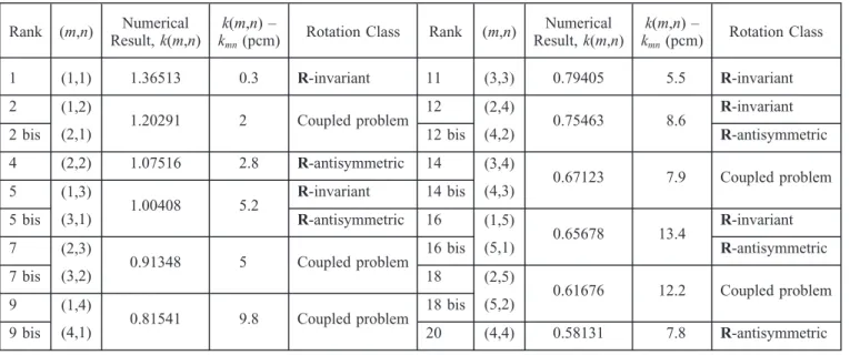
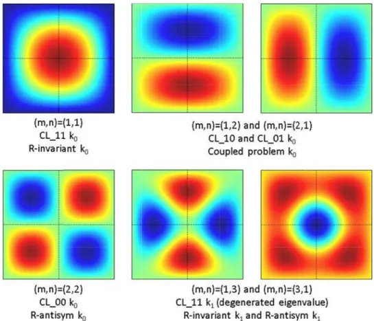
Table II lists the k-eigenvalues computed with the finite difference diffusion solver of the ERANOS code system, using the problem decomposition into rotation classes implemented according toSec. I.C.The harmonics are plotted in Fig. 2. Resolution is performed for a quarter-core using appropriate rotation boundary condi-tions (invariant, antisymmetric, coupled), and the flux obtained is subsequently unfolded for the whole core. Table II also gives the rotation class of each eigenfunc-tion. The flux harmonic ranking is obtained after complet-ing all calculations. The difference between the computed multiplication factor k(m, n) and the analytic value kmn

(see Table III) is excellent. The problem decomposition for mirror symmetry invariance (Sec. I.B), solved also for a quarter-core, but with symmetric or antisymmetric (zero flux) boundary conditions, yields exactly the same eigen-values, which is as it should be because we have used two methods to solve the same eigenvalue problem. For all calculations, the spatial mesh was 1 cm. The criteria for integral and pointwise relative convergence between the two outer or inner iterations were 10⫺8 and 10⫺6, respectively.

In the following, we use the notation CL_ab to define a symmetry class and a (respectively b) equal to 1 if the function is symmetric with respect to the x variable:

f(⫺x, y) ⫽ f(x, y) (respectively y). On the contrary, a (or b)

equals 0 if the function is antisymmetric with respect to

x (or y): f(⫺x, y) ⫽⫺f(x, y). Then, inside a symmetry class, k0is the fundamental mode, while the kiare higher modes

in that class.

Additional explanations about the degeneracies aris-ing in this problem are provided in theAppendix.

II.B. The Homogeneous Square and a Discrete

Ordinates Transport Solver

The analytical solutions of the Laplacian operator are obtained with Dirichlet conditions on the outer boundary. Such zero flux condition has no equivalent in transport theory. While the ingoing angular flux is null on this outer edge (for convex geometries, which is the case for the square), the outgoing flux is not. For homogeneous fuel material, the effect on the reactivity may reach thousands of pcm (1 pcm⫽ 10⫺5) between a void boundary tion (transport solver) and the zero flux boundary condi-tion (available in the diffusion approximacondi-tion only). To make the comparison possible, we use the extrapolation distance method. It is the distance where the flux is null in the diffusion approximation theory. Usually, this distance is small compared to the system size, and it may be neglected unless the current close to the boundary is high. In practice, we adjust the size of the square so that there is no difference between the transport solver and the analytical solution for the fundamental mode. Verification is then done comparing the high-order eigenvalues. More-over, the side of the square is progressively increased in order to estimate the difference between the transport

TABLE II

The 20 First Flux Harmonics of the Analytical Square Model and Their Rotation Classes* Rank (m,n) _{Result, k(m,n)}Numerical _kk(m,n) –

mn(pcm) Rotation Class Rank (m,n)

Numerical Result, k(m,n) k(m,n) – kmn(pcm) Rotation Class 1 (1,1) 1.36513 0.3 R-invariant 11 (3,3) 0.79405 5.5 R-invariant 2 (1,2) (2,1) 1.20291 2 Coupled problem 12 (2,4) (4,2) 0.75463 8.6 R-invariant

2 bis 12 bis R-antisymmetric

4 (2,2) 1.07516 2.8 R-antisymmetric 14 (3,4) (4,3) 0.67123 7.9 Coupled problem 5 (1,3) (3,1) 1.00408 5.2 R-invariant 14 bis 5 bis R-antisymmetric 16 (1,5) (5,1) 0.65678 13.4 R-invariant 7 (2,3) (3,2) 0.91348 5 Coupled problem 16 bis R-antisymmetric 7 bis 18 (2,5) (5,2) 0.61676 12.2 Coupled problem 9 (1,4) (4,1) 0.81541 9.8 Coupled problem 18 bis 9 bis 20 (4,4) 0.58131 7.8 R-antisymmetric *1 pcm⫽ 10⫺5.

solver and analytical solutions when the leakage becomes less significant and gradients become smoother.

Table IIIgives the first eigenvalues obtained with the transport solver. Results are obtained with a 5-cm mesh and an S8 quadrature order (80 directions). Spatial con-vergence is ensured by the discontinuous Garlerkin-based solver with a polynomial basis order fixed as uniform and equal to 2. Refined order or refined spatial mesh do not change the eigenvalues. The analytical model provides the same eigenvalue k11 provided that the extrapolation dis-tance is added on each boundary edge of the system. Then, Fig. 3 compares the absolute errors between this

extrapolated analytical model and the eigenvalues pro-vided by the transport solver.

InTable III,␭_tr⫽ 1 ⌺tot

⬇ 3 cm is the mean free path. For an infinite plane interface, the extrapolation distance is given byEq. (8):

d⬇ 0.7104/⌺tot ⫽ 0.7104 ⫻ ␭tr. (8)

One should remember that the distance in Table III is adjusted to match the result provided by the transport solver. It includes the usual extrapolation distance

Fig. 2. The shapes of the analytical solutions and their symmetry class.

TABLE III

The Five First Eigenvalues for the Transport Solver Depending on the Size of the System

Side (cm) 100 120 140 160 180 200

CL_11 k0(or k11) 1.10104 1.19489 1.26096 1.30858 1.34374 1.37030

Extrapolation distance, d (cm) 2.22 2.20 2.19 2.18 2.17 2.17

d/␭tr 0.739 0.733 0.729 0.726 0.723 0.723

CL_10/CL_01 k0(or k12); coupled problem for R 0.78919 0.91702 1.01871 1.09906 1.16267 1.21337

CL_00 k0(or k22) 0.61648 0.74513 0.85538 0.94799 1.02507 1.08903

CL_11 k1/CL_00 k1(or k13); degenerated eigenvalues 0.53869 0.66289 0.77319 0.86873 0.95034 1.01958

provided by Eq. (8) and the transport effect (since the analytical eigenvalues are those of the Laplacian operator, i.e., the diffusion equation).Table IIIshows that this model is valid especially for larger systems where the diffusion assumption is better (smooth gradients, for example).

As expected, the gaps between the calculated and the analytical values decrease with the system size. For small geometries, we may invoke a few reasons to explain why the transport solver has higher eigenvalues than the cor-responding analytical ones:

1. The diffusion approximation assumes that the flux gradients are not too high. However, since the harmonics change sign in the system, gradients may increase with the number of nodal lines.

2. The extrapolation distance is computed to match the fundamental mode. But, for higher eigenfunctions, the outgoing fluxes are greater due to the change in the flux gradients. Consequently, the fundamental flux extrapola-tion distance may not be suitable.

Anyway, the errors are always below a few hundreds pcm for the first harmonics, providing a reasonable check of the innovative boundary conditions implemented in the transport solver. Moreover, it was checked that the rota-tion problem provides the same eigenvalues as the sym-metry problems. These eigenvalues are also those that were computed on the full-core system.

II.C. The Homogeneous Regular Hexagon and a

Discrete Ordinates Transport Solver

The elementary assembly is a regular hexagon. Its pitch h equals 13 cm (its side A equals 7.5 cm). This element is repeated in several rings to define a larger geometry. We progressively increase the number of rings (this number includes the central hexagon). The final core

models a large regular hexagon. This geometry is invari-ant under an order-6 rotation and in fact is also invariinvari-ant under action of the noncommutative symmetry group

C_6v ⫽ 兵I, R, R2_{, R}3_{, R}4_{, R}5_{, S}

0, S1, S2, S3, S4, S5其 (see Fig. 4). However, as explained above, we limit ourselves to the order-3 rotation R decomposition problem.

For verification purposes, we use the eigenvalues of the Laplacian over a regular hexagon computed in Ref. 11.Equation (9)gives the expression of the eigenvalues for a regular hexagon of side A:

⌬ui ⫹ ␭i A2ui ⫽ 0 ; ki ⫽ k_⬁ 1⫹ M2␭i A2 . (9)

Numerical values are given inTable IV(for A⫽ 1 cm), and the corresponding shapes are printed inFig. 5.␭0,␭3,

Fig. 3. Difference between Sn solver and analytical model on the first eigenvalues for the homogeneous square.

Fig. 4. Cross section of a prismatic hexagonal homoge-neous system with trace of the mirror symmetry planes (⌸0through⌸5), with␲/6 clockwise angle between one

and the next. R⫽ S0S2is the counterclockwise rotation of

␭4, and ␭5belong to R-invariant functions, while ␭1,␭2, and␭6come from the coupled problem and are degener-ated (of order 2).

As for the homogeneous square, the Dirichlet con-ditions on the outer boundary cannot be used in the Sn solver. Moreover, there is a tiny gap between both geometries (one regular hexagon for the analytical model instead of several rings of elementary hexagons

for the Sn solver). To make the comparison possible, the analytical side A (or equivalently the pitch H) is adjusted to match the fundamental eigenvalue provided by the Sn solver. Results are gathered in Table V. Then, the verification is done on higher harmonics (see Fig. 6).

Based onFig. 6, the conclusions are similar to those given for the homogeneous square.

TABLE IV

Some Eigenvalues of the Regular Hexagon (of 1-cm Side) with Dirichlet Boundary Conditions*

␭0 ␭1 ␭2 ␭3 ␭4 ␭5 ␭6

R-Invariant Coupled Problem Coupled Problem R-Invariant R-Invariant R-Invariant Coupled Problem

7.15534 18.13168 32.45186 37.49136 47.62937 52.63789 60.10516

*All functions are the eigenmodes of the Laplacian operator (fromRef. 11).

Fig. 5. The shapes of the first eigenvalues for the homogeneous hexagon. The top row comes for R-invariant modes. The bottom row is the result of the coupled problem (only for␭1and␭2).

TABLE V

The Eigenvalues Obtained with the Transport Solver for the Regular Homogeneous Hexagon

Number of rings 6 7 8 9 10 11 R-invariant, k0(␭0) 1.18626 1.25935 1.31062 1.34763 1.37504 1.39583 Pitch H (analytical) (cm) 127.5 150.0 172.5 195.0 217.5 240.0 R-invariant, k1(␭3) 0.62872 0.74953 0.85369 0.94196 1.01615 1.07834 R-invariant, k2(␭4) 0.54338 0.66021 0.76460 0.85586 0.93463 1.00216 Coupled problem, k0(␭1) 0.89810 1.01063 1.09798 1.16595 1.21923 1.26145 Coupled problem, k1(␭2) 0.68197 0.80357 0.90617 0.99154 1.06221 1.12068 Coupled problem, k2(␭6) 0.46560 0.57577 0.67759 0.76933 0.85065 0.92200

II.D. Conclusions of the Verification Work

The innovative boundary conditions described in the companion paper10 _{were implemented in an Sn}

solver and 2-D Cartesian diffusion solver. Advantage was taken from the currently implemented boundary conditions (reflective, periodic) so that only a few changes were needed (except for the coupled problem). Some analytical solutions of the Laplacian operator were compared to the eigenvalues obtained in the trans-port theory. Some differences may appear between both approaches due to the treatment of leakage (outer boundary condition) and to the transport effect. How-ever, we adjusted the extrapolation distance (or equiv-alently the size of the analytical model) to match the fundamental mode. Then, it is possible to compare directly the higher eigenvalues. Results are excellent for both the integral values and the shapes. Further verification work could include Monte Carlo capability to produce a fission matrix.12,13

InSec. III, we propose to compute the first harmonics of the Takeda benchmark.14

III. THE HARMONICS FOR THE TAKEDA BENCHMARK

III.A. Takeda Model 1

The first model of the Takeda benchmark is a small homogeneous pressurized water reactor reflected core.14

In case 1, the control rods (CRs) are withdrawn and replaced by a void medium whereas they are completely inserted in case 2. The two-group cross sections are

provided, and a 1-⫻ 1- ⫻ 1-cm reference Cartesian mesh is used. One-quarter symmetries have been accounted, which allow the use of innovative reflective boundary conditions. The minimal sector to be defined for the com-putation is a one-eighth core.

To define the harmonics, we use the following rules. First, we define a symmetry class (of functions) noted CL_abc; a (respectively b and c) equals 1 if the function is symmetric with respect to the x variable f(⫺x,y,z) ⫽

f(x,y,z) (respectively y and z) and equals 0 if the function

is antisymmetric with respect to x: f(⫺x,y,z) ⫽ ⫺f(x,y,z) (respectively y and z). Second, inside each class, we note the fundamental mode k0 and higher harmonics ki.

Basi-cally, the k0 of class CL_111 is the fundamental-mode eigenvalue while the k0of class CL_110 is the first axial harmonic eigenvalue.

Results are gathered inTable VI, which also gives the reference Monte Carlo TRIPOLI-4 (Ref. 15) results.16_For

the Sn solver, an S6 level-symmetric angular quadrature is enough to match the reference Monte Carlo calculation. The polynomial basis order p of the DG scheme is fixed as uniform, and p ⫽ 2. In Table VI, it can be noticed that there is no degeneracy in this system.

III.B. Takeda Model 2

The second Takeda model is a homogeneous fast breeder reactor (FBR) with axial and radial blankets. The reference mesh size is 5 ⫻ 5 ⫻ 5 cm. Two cases are considered. In case 1, the CR is withdrawn and replaced by Na. In case 2, the CR is half inserted. In this second case, the geometry is no longer invariant under the

z-axis symmetry. The minimal sector to be defined is a

quarter-core.

The symmetry class is noted CL_ab (since there is no more symmetry with respect to the z-axis). The first axial harmonic will appear in the class of symmetric functions with respect to the x-axis and y-axis. For both cases, this axial harmonic corresponds to CL_11 k1. In case 1, sym-metric with respect to the z variable, one may compute the flux harmonics on one-eighth of the core, and then, this axial harmonic is obtained as the fundamental mode of symmetry class CL_110. However, in case 2, one has to model at minimum one-quarter of the core, and therefore, the axial harmonic belongs to class CL_11 and is obtained as the first harmonic of this class. The second harmonic corresponding to CL_111 k1 of case 1 (or equivalently CL_11 k2) requires the filtering by two functions, and convergence is difficult to achieve. In Table VII, the italicized values correspond to eigenvalues where integral convergence (10⫺5) is satisfied, but pointwise conver-gence (10⫺4) is not achieved even after 100 outer iterations.

The core calculation is performed in four groups. An S6 level-symmetric angular quadrature is used, and the polynomial basis order p of the DG scheme is fixed as uniform p⫽ 2.

Among these eigenvalues, it is remarkable to observe the behavior of CL_10 k0 and CL_01 k0 between both cases. The CR is inserted near the x-axis, which is a nodal line for the CL_10 k0mode. Thus, the CR move does not change either this eigenvalue or the shape of this har-monic. On the contrary, harmonic CL_01 reaches a max-imum near this CR and will be strongly excited by its move. This will affect the shape of the power distribution and is extensively studied.17,18_{In a few words, the}

knowl-edge of the flux harmonics may help to optimize the core design, and this will be the subject of future work.

III.C. Takeda Model 3

The third Takeda model is a heterogeneous Cartesian FBR core with internal/external blankets and radial/axial reflectors. A 5-⫻ 5- ⫻ 5-cm mesh interval in the one-eighth core model is the reference mesh size. Four-group cross sections are used for calculations. Finally, three cases are considered. In case 1, CRs are inserted. In case 2, they are removed. In case 3, they are replaced with core and/or blanket cells.

In this model, an S6 quadrature order was used. In this case, we can take advantage of the local-p refine-ment capability offered by the DG spatial scheme. In all

TABLE VI

The First Eigenvalues for Takeda Benchmark Model 1 Case 1 (CR Withdrawn, Void) Case 2 (CR Inserted) TRIPOLI-4 (fundamental) 0.97729⫾ 0.00002 (1␴) 0.96240⫾ 0.00002 (1␴) CL_111 k0(fundamental) 0.97719 0.96244 CL_111 k1 0.46317 0.46380 CL_101 k0(nodal line y⫽ 0) 0.70040 0.70177 CL_011 k0(nodal line x⫽ 0) 0.68054 0.65174 CL_001 k0(nodal lines x⫽ 0; y ⫽ 0) 0.52863 0.53114 CL_110 k0(nodal line z⫽ 0) 0.69324 0.68911 TABLE VII

The First Eigenvalues for Takeda Benchmark Model 2 Case 1 (CR Withdrawn, Void) Case 2 (CR Inserted) TRIPOLI-4 (fundamental) 0.97368⫾ 0.00002 (1␴) 0.95968⫾ 0.00002 (1␴) CL_11 k0 0.97364 0.95961 CL_11 k1(axial harmonic) 0.77133 0.76415 CL_11 k2 0.56825 0.56530 CL_10 k0 0.75055 0.75177 CL_01 k0 0.73366 0.71140 CL_00 k0 0.57663 0.57943

materials, p⫽ 2 except in the empty Matrix and radial reflector subassemblies where p ⫽ 1. This allows the number of degrees of freedom (see Ref. 8 for more details) to be reduced from 497 664 for a full (p ⫽ 2) computation to 380 244 for this variable first/second spatial order. This is enough to match the Monte Carlo reference.

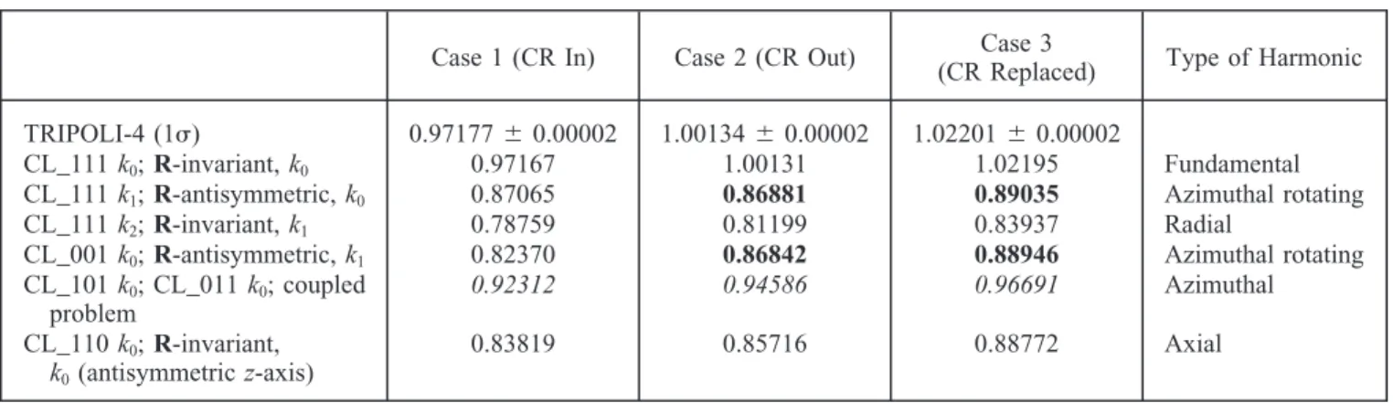
This geometry is again Cartesian, and the innovative reflective boundary conditions can be used. But, the model is also invariant under an order-4 rotation, which leads to some degeneracy in the eigenmodes. We keep the same nomenclature to define the symmetry classes and add the rotation class inTable VIII. The right column also gives the type of harmonic with respect to the notation of Verdu et al.19 _{This example illustrates that the search of}

harmonics can be easier by solving several fundamental modes and thus avoiding the filtering technique. More-over, the relative dominant ratio inside a given class can be significantly increased.

In Table VIII, the italicized values are degenerated because the geometry is invariant under an order-4 rota-tion. Corresponding harmonics may be computed as fun-damental modes of symmetry classes CL_101 and CL_011 or as the coupled solutions of the rotation prob-lem. The boldfaced values are almost degenerated (in the 50-pcm range). Both eigenfunctions are azimuthal rotat-ing harmonics, belongrotat-ing to the R-antisymmetric class. However, it is remarkable to see that after the insertion of the CR (case 1), both eigenvalues are split. In fact, the CL_111 k1 harmonic is null over the five inserted CRs, which explains why this eigenvalue is about the same whether the CRs are withdrawn or not. On the contrary, the CL_001 k0harmonic reaches maximum values in these CR positions: When the CRs are inserted, the eigenvalue changes considerably.

For the shapes of the corresponding harmonics, please refer toFig. 8 inSec. IV.

III.D. Takeda Model 4

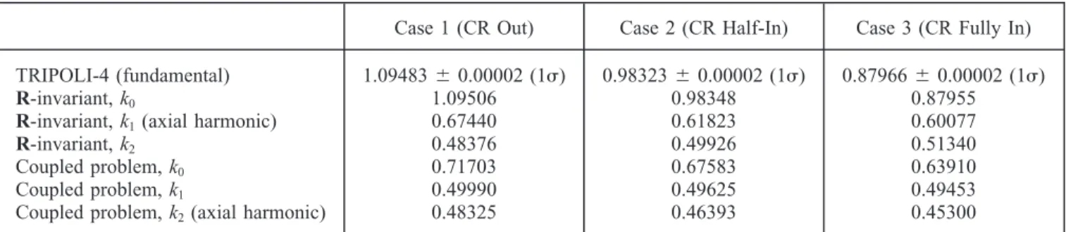
The fourth Takeda model is a heterogeneous hexagonal-z FBR core with strong radial (eight fuel rings and reflector) and axial (blanket, CR, and reflector) heterogeneities, coming from the KNK-II core. There are three configurations depending on the CR positions. In case 1, all CRs are out and then they are half inserted in case 2 and are fully inserted in case 3.

The model is invariant under an order-6 rotation operator. However, for the sake of analysis of the new sodium fast reactor (SFR) design, we treat only one-third of the full core (order-3 rotation invariance). We solve the eigenvalue problem for the R-invariant functions and for the coupled problems. Each harmonic is noted ki, with i

indicating the rank of the harmonic in the rotation class (see Table IX). As explained by Le Tellier et al.,8 _a

third/second spatial order is used for the polynomial basis. For the angular quadrature order, a product quadrature is constructed by symmetry from an azimuthal quadrature based on an Na-point Gauss-Chebychev rule on [0, ␲/3]

and a polar quadrature based on an Np-point

Gauss-Legendre rule on [0, 1]. It is denoted HQNa,Np and has

12⫻ Na ⫻ Np points over the complete unit sphere (see Ref. 8for more details). In this work, HQ3,2 was chosen. In this benchmark, azimuthal rotating harmonics may be higher order than axial harmonics because of the height of the geometry compared to its radial size. In the R-invariant class, the flux harmonic k1 is axial, while k2 is the radial eigenfunction (similar to ␭3 inSec. II.C). For the coupled problem, the k2eigenvalue is an axial mode (its sign changes over the z-axis). In fact, for large cores of relatively small height (such as the new design for a low-void-effect core), the azimuthal harmonic eigenvalues will be higher than the axial harmonic eigenvalues. This is not the case for this Takeda benchmark. However, for the sake of our objective, which was to compute some flux harmonics on various geom-etries with invariance properties, this is not really a concern.

TABLE VIII

The First Eigenvalues for Takeda Benchmark Model 3

Case 1 (CR In) Case 2 (CR Out) _{(CR Replaced)}Case 3 Type of Harmonic

TRIPOLI-4 (1␴) 0.97177⫾ 0.00002 1.00134⫾ 0.00002 1.02201⫾ 0.00002

CL_111 k0; R-invariant, k0 0.97167 1.00131 1.02195 Fundamental

CL_111 k1; R-antisymmetric, k0 0.87065 0.86881 0.89035 Azimuthal rotating

CL_111 k2; R-invariant, k1 0.78759 0.81199 0.83937 Radial

CL_001 k0; R-antisymmetric, k1 0.82370 0.86842 0.88946 Azimuthal rotating

CL_101 k0; CL_011 k0; coupled problem 0.92312 0.94586 0.96691 Azimuthal CL_110 k0; R-invariant, k0(antisymmetric z-axis) 0.83819 0.85716 0.88772 Axial

IV. APPLICATION EXAMPLE: THE ZPPR-18A

EXPERIMENTAL CORE

The case studied here is a three-dimensional geome-try inspired by the ZPPR-18A benchmark20_{(seeFig. 7for}

a cross cut at the core midplane). It corresponds to the critical reference benchmark. This core is an engineering mock-up critical experiment of a 1000-MW(electric)– class sodium-cooled mixed oxide–fueled FBR core with two homogeneous zones with enriched uranium in the

TABLE IX

The First Eigenvalues for Takeda Benchmark Model 4

Case 1 (CR Out) Case 2 (CR Half-In) Case 3 (CR Fully In)

TRIPOLI-4 (fundamental) 1.09483 ⫾ 0.00002 (1␴) 0.98323⫾ 0.00002 (1␴) 0.87966⫾ 0.00002 (1␴)

R-invariant, k0 1.09506 0.98348 0.87955

R-invariant, k1(axial harmonic) 0.67440 0.61823 0.60077

R-invariant, k2 0.48376 0.49926 0.51340

Coupled problem, k0 0.71703 0.67583 0.63910

Coupled problem, k1 0.49990 0.49625 0.49453

Coupled problem, k2(axial harmonic) 0.48325 0.46393 0.45300

outer core region and all CRs are fully withdrawn to simulate the end of operating cycle condition.

As for our concern, one can model one-eighth of the core and then unfold the flux harmonics using the innovative boundary conditions. Since the reactor is not invariant by rotation, degeneracies are not expected. We first solve the diffusion equation with 33 energy groups in the ERANOS platform. This provides an opportunity to discuss the relative EVSs that might be computed depend-ing on the symmetry class considered. Then, the first eigenvalues of the transport equation are computed using the discrete ordinates solver SNATCH.

IV.A. The Harmonics of the Diffusion Equation

We start searching for the flux harmonics of the mul-tigroup diffusion equation either for the full geometry or for a one-eighth core. In the latter, we keep the same conventions to define a symmetry class, which is noted CL_abc; a (respectively b and c) equals 1 if the function is symmetric with respect to the x variable f(⫺x,y,z ⫽

f(x,y,z) (respectively y and z), and a (respectively b and c)

equals 0 if the function is antisymmetric with respect to the x variable f(⫺x,y,z) ⫽ ⫺f(x,y,z) (respectively y and z). The symmetry operation deals only with the spatial vari-able since the angular varivari-able disappears in the diffusion approximation.

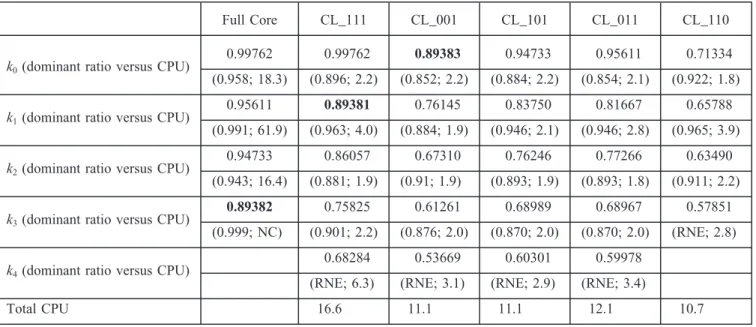
Table Xgives the first eigenvalues of each symmetry class. It provides also the dominant ratio, defined as

k_i⫹1/k_i. The convergence speed of the power iteration method is controlled by this parameter. Thus, Table X gives the CPU time needed to converge for each eigen-function. The integral convergence criterion is 0.5 pcm, while the pointwise criterion is 10⫺5 (relative conver-gence). This time strongly depends on the initial guess used to initialize the power iteration method. For the one-eighth core, the initial guess was a vector all of whose components were 1 (uniform distribution). How-ever, for the full-core computation, the initial guess for the power iteration method must have projections over all eigenmodes. To satisfy this condition, we used as an initial vector the fundamental mode of a modified geometry (one CR inserted while the others are still withdrawn). Such distribution ensures having projections over all eigenmodes (or all symmetry classes). The CPU times are given to illus-trate the highly improved performance of the reduced-size problems, and they are not necessarily transposable directly to other cases (especially because they depend on the initial guess used).

A CPU time of 18.3⫻ 103 _{s is required to compute} the fundamental mode over the full core, while 16.6⫻ 103_s is enough to provide about 25 flux harmonics if reduced-size problems (one-eighth core with appropriate boundary condi-tions) are computed on parallel computers. This difference is explained by the following:

1. the size of the geometry to be modeled, especially for the inner process (once the fission source is known), which requires the inversion of a large

TABLE X

Eigenvalue, Dominant Ratio (DR⫽ ki⫹1/ki), and CPU Time Needed (⫻1000 s) to Compute

the Harmonics Depending on the Reduced-Size Problems; Diffusion Solver*

Full Core CL_111 CL_001 CL_101 CL_011 CL_110

k0(dominant ratio versus CPU)

0.99762 0.99762 0.89383 0.94733 0.95611 0.71334

(0.958; 18.3) (0.896; 2.2) (0.852; 2.2) (0.884; 2.2) (0.854; 2.1) (0.922; 1.8)

k1(dominant ratio versus CPU)

0.95611 0.89381 0.76145 0.83750 0.81667 0.65788

(0.991; 61.9) (0.963; 4.0) (0.884; 1.9) (0.946; 2.1) (0.946; 2.8) (0.965; 3.9)

k2(dominant ratio versus CPU)

0.94733 0.86057 0.67310 0.76246 0.77266 0.63490

(0.943; 16.4) (0.881; 1.9) (0.91; 1.9) (0.893; 1.9) (0.893; 1.8) (0.911; 2.2)

k3(dominant ratio versus CPU)

0.89382 0.75825 0.61261 0.68989 0.68967 0.57851

(0.999; NC) (0.901; 2.2) (0.876; 2.0) (0.870; 2.0) (0.870; 2.0) (RNE; 2.8)

k4(dominant ratio versus CPU)

0.68284 0.53669 0.60301 0.59978

(RNE; 6.3) (RNE; 3.1) (RNE; 2.9) (RNE; 3.4)

Total CPU 16.6 11.1 11.1 12.1 10.7

sparse matrix; reducing the size of such matrices considerably improves the speed of convergence 2. the artificially increased dominant ratio inside

each symmetry class.

This illustrates the advantage, for symmetric cores, to partition the problem into symmetry classes with appropriate boundary conditions. Moreover, the k3harmonic of the full core (boldface eigenvalue inTable X) does not satisfy point-wise convergence even after 400 outer iterations. It is prob-ably due to the pseudodegeneracy between both azimuthal rotating flux harmonics. So, reduced-size problems allow the computation of more harmonics than the traditional filtering technique applied in full-core geometry.

The first six eigenfunctions are plotted in Fig. 8. The plots represent the scalar flux, integrated over all energy groups and over the axial direction. In this flat core, the first axial harmonic has a very higher-order rank. This means that all printed harmonics are azimuthal or radial (i.e., the flux does not change sign in the axial direction). The type of harmonic comes from the notation used by Verdu et al.19

Depending on the initial guess (or on the assumptions of the solver), at least three eigenvalue-separations can be inferred based on these harmonics:

1. The real EVS must be calculated using the real first harmonic (in the decreasing ranking of eigenvalues).

Here, EVS ⫽ k0k1

k0⫺ k1

⫽ 23.0 (or equivalently ε ⫽

k0⫺ k1

k₀ ⫽ 4.16%), which is very close to the value given

by Sanda et al.22 _{(4.18%). In Ref. 22, the static flux tilt}

method is used to measure experimentally the EVS. 2. If harmonics are computed in the reduced-size (quarter-core) problem but use the standard reflection boundary condition only, the fourth mode will be obtained, leading to EVS ⫽ k0k4

k0⫺ k4

⫽ 8.6 (or ε ⫽ 10.4%). This value can also be obtained for the full reactor if the initial vector is symmetric and the conver-gence criteria are not tight enough.

3. If the reactor had been cylinderized and then calculated in RZ geometry, the computed EVS would have been close to EVS⫽ k0k5

k₀⫺ k5 ⫽ 6.3 (or ε ⫽ 13.7%). In

this ZPPR case, because of the Pu/U outer zones, such a cylindrical model is not well adapted, but the Japan Atomic Energy Agency benchmark proposed one.

IV.B. The Harmonics of the Transport Equation

This section aims at providing the five first harmonics of the ZPPR-18A critical configuration for the transport

equation. In order to do that, we use the discrete ordinates discontinuous Galerkin-based solver SNATCH. The spa-tial mesh is 5.5 ⫻ 5.5 cm radially, and axial meshes are ⬃5 cm (in the finite difference diffusion solver, it was ⬃2.5 cm).

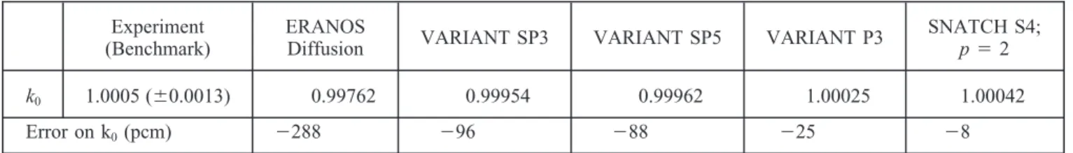
First, we evaluate the performance of the SNATCH solver. The polynomial basis degree p of the DG scheme equals 2 for fuel regions and is released (to 1) in the empty matrix region; radial reflectors and upper axial reflectors are as suggested in Ref. 8. An S4 quadrature order was used (24 directions).Table XIgathers all results.Table XI also gives the results obtained with the nodal variational solver VARIANT of the ERANOS platform23_{for several}

orders of flux expansion order (over the spherical harmon-ics). This solver uses spherical harmonics, and the mac-roscopic cross sections are identical to those used in SNATCH. Simplified P3 (SP3) means that the Pn method is used with order-3 and that we keep only a fraction of the angular expansion.

Table XI shows good agreement among all codes used. The transport effect for the fundamental mode is ⬃280 pcm for this relatively large core (with radial and axial blankets). The simplified spherical harmonics method reduces the error on the eigenvalue below 100 pcm. The discrete ordinates method provides the best result, and the choice of S4 angular quadrature and sec-ond/first polynomial basis order seems enough to match the experimental value. Traverses along the x-axis and

y-axis were compared between this codes for the

micro-scopic fission rate of235_{U (for all traverses, z}⫽ 5 cm). The

traverses are normalized so that the 235_{U-fission rates at} the assembly center are equal for all codes (and identical to those provided by the benchmark). The VARIANT and the SNATCH traverses are almost identical. Averaged calculated-to-experimental (C/E) values per zone are given in Table XII. The diffusion solver underestimates the flux in the outer core and radial blankets along the

x-axis, but these differences are reduced with the transport

solver. For the Y-traverses crossing the enriched uranium outer core, both codes present accurate results compared to the experimental traverses.

For our purpose (compute the first eigenvalues of the transport equations), the choice of variable first/second

p-order and symmetric level S4 angular quadrature seems

enough. Results are given in Table XIII for the first eigenvalues. The transport effect (⫹280 pcm for the fun-damental mode) is higher for all harmonics, especially for the first axial mode. In fact, each harmonic is a “kind of fundamental mode” over a reduced geometry: It would be approximately the physical solution of the neutron trans-port equation if we build half a reactor. The only differ-ence is the antisymmetric boundary conditions (see Sec. I.B), which are different from the traditional void condition. But for small geometries (with significant gradients), the diffusion is not well adapted, which explains why the transport effect is increased. To com-pute a higher harmonic, a transport solver seems more efficient than a diffusion one.

The traverses along the x-axis for the CL_011 k0 harmonic and the traverses along the y-axis for the

TABLE XI

The Fundamental-Mode Eigenvalues Provided by Several Solvers for the ZPPR-18A Benchmark Experiment

(Benchmark)

ERANOS

Diffusion VARIANT SP3 VARIANT SP5 VARIANT P3

SNATCH S4;

p⫽ 2

k0 1.0005 (⫾0.0013) 0.99762 0.99954 0.99962 1.00025 1.00042

Error on k0(pcm) ⫺288 ⫺96 ⫺88 ⫺25 ⫺8

TABLE XII

Averaged C/E and Standard Variation (1␴) for Microscopic235_{U Fission Rate Traverse}

Between Deterministic Codes and Experimental Benchmark Values

Traverse Zone Diffusion Solver SNATCH Solver

x-axis Inner core

Outer core⫹ radial blanket

0.995⫾ 0.011

0.968⫾ 0.013

1.000⫾ 0.007

0.984⫾ 0.014

y-axis Inner core

Outer core (U-zone)

0.999⫾ 0.012

0.998⫾ 0.018

1.000⫾ 0.011

CL_100 k0 harmonic are illustrated in Fig. 9 for the diffusion solutions and the discrete ordinates transport solver. The traverses are normalized so that their respec-tive maxima equal 1. In Fig. 9, it can be seen that the shapes of the harmonics are about the same for diffusion and transport harmonics (the SNATCH/diffusion ratio is always within a 1% range of 1). For example, the peaks of the flux harmonics are around the same assembly. All discrepancies have the same magnitude as those observed when we compare the experimental traverses and the fundamental modes (⬃2% to 3%).

V. CONCLUSIONS

In the present work, we implement in existing solvers the theory described in a companion paper for computing the flux harmonics of nuclear systems characterized by some invariance properties. After recalling the main conclusions of the previous work, we verify simplified geometrical shapes, such as a homogeneous square and a regular hexagon. For that purpose, new versions based on the existing finite difference diffusion solver of the ERANOS platform and on a discontinuous Garlerkin-based transport solver (discrete ordinates) called SNATCH have been developed. In monokinetic conditions, the flux

harmonics may be approached by a series of eigenfunc-tions of the Laplacian operator. Extrapolation distance is used to test the newly developed transport solver against analytical solutions.

Once the new capabilities of the code are tested, the transport flux harmonics of the Takeda benchmarks are computed using the SNATCH code. Results are briefly commented upon, and some applications of high-order harmonics are suggested. This will be the topic of future work, especially when linking the power distribution sen-sitivity to the EVS in a large SFR.

Finally, the flux harmonics of the ZPPR-18A exper-iment are computed both by the modified ERANOS dif-fusion solver and the modified SNATCH Sn solver. With the diffusion approximation, the interests of reduced-size decomposition problems are highlighted.Section IValso deals with the main EVS values that could be computed depending on the choice of boundary conditions being used and the resulting type of harmonic—azimuthal, axial, radial—that can be accessed.

Finally, using innovative boundary conditions for the Sn solver, we are able to access the same harmonics. Eigenvalues and shapes of the flux harmonics of the two solvers are compared with one another. For that purpose, traverses along the x-axis and the y-axis between diffusion

TABLE XIII

The First Eigenvalues for All Symmetry Classes of ZPPR-18A Benchmark Provided by the Diffusion Solver and SNATCH*

CL_111 k0 CL_001 k0 CL_101 k0 CL_011 k0 CL_110 k0

Type of harmonic Fundamental Azimuthal rotating Azimuthal Azimuthal Axial

Diffusion 0.99762 0.89383 0.94733 0.95611 0.71334

SNATCH 1.00042 0.89874 0.95063 0.96011 0.72170

Transport effect (pcm) ⫹280 ⫹491 ⫹330 ⫹400 ⫹836

*The transport effect is defined as the difference between SNATCH eigenvalue and the diffusion one.

Fig. 9. Traverses along x-axis (for CL_011 harmonic) and y-axis (for CL_101 harmonic) for the235_{U microscopic fission rate}

eigenfunctions and corresponding transport eigenfunc-tions are compared. It seems that the diffusion harmonics are a good approximation of equivalent transport harmon-ics, at least for the very first eigenfunctions. Complemen-tary work needs to be done to confirm this trend. This could possibly be done using the Monte Carlo code capa-bility to build the fission matrix over refined spatial meshes. In this approach, taking into account the invari-ance properties allows the reduction of the system size to be modeled, which is a major advantage of the fission matrix computation. However, this requires implementing innovative boundary conditions in Monte Carlo codes. Once such fission matrices are computed, we are able to simultaneously compute hundreds of harmonics. These eigenfunctions could then define an expansion basis to be used to reconstruct any perturbed flux, using traditional perturbation theory.

APPENDIX

ANALYTICAL SOLUTION FOR MONOENERGETIC

DIFFUSION IN THE HOMOGENEOUS SQUARE

Action of the symmetry operations on the ␹2

eigen-functions Smnis easily checked to be as follows:

兵

兵

1. If m and n share the same parity, (m⫹ n) is even, and R2_S

mn ⫽ Smn. We can construct two eigenfunctions

based on Smn and Snm, corresponding to the same

eigen-value determined by the sum (m2⫹ n2_{); seeEq. (7):}

a⫽ Smn⫹ Snmverifies Ra ⫽ a

and

b⫽ Smn⫺ Snmverifies Rb ⫽ ⫺b .

An example of such degeneracy is provided by S13 and S31.

2. If m and n do not have the same parity, then (m⫹ n) is odd, and R2_S

mn⫽ ⫺Smn. Here, we construct two

eigen-functions by

u⫽ Smn

and

v ⫽ (⫺1)n_S nm

so that u and v verify

兵

Rv⫽ u , which is the expression

of the coupled problem for the rotation class. An example of such degeneracy is provided by S12and S21.

References

1. T. E. BOOTH, “Power Iteration Method for the Several Largest Eigenvalues and Eigenfunctions,” Nucl. Sci. Eng.,

154, 48 (2006);http://dx.doi.org/10.13182/NSE05-05. 2. G. B. BRUNA and A. SARGENI, “A Computational

Tech-nique for Evaluating Eigenfunctions of Symmetrical Nuclear Systems,” Ann. Nucl. Energy, 21, 12, 745 (1994);

http://dx.doi.org/10.1016/0306-4549(94)90023-X.

3. G. RIMPAULT et al., “ERANOS Code and Data System for Fast Reactor Neutronic Analyses,” Proc. PHYSOR

2002, Seoul, Korea, October 7–10, 2002.

4. R. S. MODAK and A. GUPTA, “Use of a New Boundary Condition in Computational Neutron Transport,” Nucl. Sci.

Eng., 163, 263 (2009);http://dx.doi.org/10.13182/NSE163-263. 5. Y. KATO et al., “Analysis of First-Harmonic Eigenvalue

Separation Experiments on KUCA Coupled Core,” J. Nucl.

Sci. Technol., 35, 3, 216 (1998);http://dx.doi.org/10.1080/ 18811248.1998.9733847.

6. D. E. KORNREICH and D. K. PARSONS, “Diffusion and Transport Analysis of Higher Mode Eigensystems,” Proc.

Int. Conf. Nuclear Mathematical and Computational Sci-ences, Gatlinburg, Tennessee, April 6 –11, 2003.

7. F. VARAINE et al., “Pre-Conceptual Design Study of ASTRID Core,” Proc. Int. Congress Advances in Nuclear

Power Plants (ICAPP), Chicago, Illinois, June 24 –28,

2012, American Nuclear Society (2012).

8. R. LE TELLIER et al., “High-Order Discrete Ordinate Transport in Hexagonal Geometry: A New Capability in

ERANOS,” Il Nuovo Cimento C, 33, 1, 121 (2010);http://

dx.doi.org/10.1393/ncc/i2010-10565-5.

9. R. LE TELLIER, D. FOURNIER, and C. SUTEAU, “Reac-tivity Perturbation Formulation for a Discontinuous Galerkin-Based Transport Solver and Its Use with Adaptive Mesh Refinement,” Nucl. Sci. Eng., 167, 209 (2011);http:// dx.doi.org/10.13182/NSE10-34.

10. J. TOMMASI, M. MAILLOT, and G. RIMPAULT, “Cal-culation of Higher-Order Fluxes in Symmetric Cores—I: Theory,” Nucl. Sci. Eng., 184, 174 (2016);http://dx.doi.org/ 10.13182/NSE16-4.

11. L. M. CURETON and J. R. KUTTLER, “Eigenvalues of the Laplacian on Regular Polygons and Polygons Resulting from Their Disection,” J. Sound Vib., 220, 1, 83 (1999);

12. T. KITADA and T. TAKEDA, “Evaluation of Eigenvalue Separation by the Monte Carlo Method,” J. Nucl. Sci.

Tech-nol., 39, 2, 129 (2002);http://dx.doi.org/10.1080/18811248. 2002.9715166.

13. S. CARNEY et al., “Theory and Application of the Fission Matrix Method for Continuous-Energy Monte-Carlo,” Ann.

Nucl. Energy, 73, 423 (2014); http://dx.doi.org/10.1016/j. anucene.2014.07.020.

14. T. TAKEDA and H. IKEDA, “3-D Neutron Transport Benchmarks,” NEACRP-L-330, Organisation for Eco-nomic Co-operation and Development/Nuclear Energy Agency, Committee on Reactor Physics (1991).

15. E. BRUN et al., “TRIPOLI-4®, CEA, EDF and AREVA Reference Monte Carlo Code,” Ann. Nucl. Energy, 82, 151 (2015);http://dx.doi.org/10.1016/j.anucene.2014.07.053. 16. J.-M. PALAU et al., “Recent Advances in the V&V of the

New French CEA APOLLO3® Neutron Transport Code: Benchmarks Analysis of the Flux Solvers,” Proc. Int. Conf.

PHYSOR 2014, Kyoto, Japan, September 28 –October 3,

2014.

17. A. SARGENI, K. W. BURN, and G. B. BRUNA, “Cou-pling Effects in Large Reactor Cores: The Impact of Heavy and Conventional Reflectors on Power Distribution Pertur-bations,” Proc. Int. Conf. PHYSOR 2014, Kyoto, Japan, September 28 –October 3, 2014.

18. G. RIMPAULT et al., “Flux Harmonics in Large SFR Cores in Relation with Core Characteristics Such as Power Peaks,” Proc. Int. Conf. Nuclear Mathematical and

Com-putational Sciences (M&C 2013), Sun Valley, Idaho, May

5–9, 2013, American Nuclear Society (2013).

19. G. VERDU et al., “3D␭-Modes of the Neutron-Diffusion

Equation,” Ann. Nucl. Energy, 21, 7, 405 (1994);http://dx. doi.org/10.1016/0306-4549(94)90041-8.

20. T. SANDA, M. ISHIKAWA, and R. M. LELL, “ZPPR-18A Experiment: A 1,000 MWe-Class Sodium-Cooled MOX-Fueled FBR Core Mock-Up Critical Experiment with Two-Homogeneous Zones and Control-Rod Withdrawal, Where Enriched Uranium Is Used with the Shape of a Sector in the Outer Core,” ZPPR-LMFR-EXP-003, CRIT-SPEC-REAC-RRATE-MISC, NEA/NSC/DOC(2006)1, Organisation for Economic Co-operation and Development/Nuclear Energy Agency, Nuclear Science Committee (2006).

21. T. SANDA, M. ISHIKAWA, and R.D. McKNIGHT, “ZPPR-18C Experiment: A 1,000 MWe-Class Sodium-Cooled MOX-Fueled FBR Homogeneous Core Mock-Up Critical Exper-iment in the State of Removal of One of Eighteen Half-Inserted Control Rods, Where Enriched Uranium is Used with the Shape of a Sector in the Outer Core,” ZPPR-LMFR-EXP-008, CRIT-SPEC-RRATE, NEA/NSC/DOC(2006)1, Organisation for Eco-nomic Co-operation and Development/Nuclear Energy Agency, Nuclear Science Committee (2006).

22. T. SANDA, F. NAKASHIMA, and K. SHIRAKATA, “Neutronic Decoupling and Space-Dependent Nuclear Characteristics for Large Liquid-Metal Fast Breeder Reac-tor Cores,” Nucl. Sci. Eng., 113, 97 (1993); http://dx.doi. org/10.13182/NSE113-97.

23. E. E. LEWIS, M. A. SMITH, and G. PALMIOTTI, “The Variational Nodal Method: Some History and Recent Activ-ity,” Proc. Int. Conf. Nuclear Mathematical and Computation,

Supercomputing, Reactor Physics and Nuclear and Biological Applications, Avignon, France, September 12–15, 2005.