Dating groundwater with dissolved silica and CFC concentrations in crystalline aquifers

(1)

HAL Id: insu-01779877

https://hal-insu.archives-ouvertes.fr/insu-01779877

Submitted on 27 Apr 2018

HAL is a multi-disciplinary open access archive for the deposit and dissemination of sci-entific research documents, whether they are pub-lished or not. The documents may come from teaching and research institutions in France or abroad, or from public or private research centers.

L’archive ouverte pluridisciplinaire HAL, est destinée au dépôt et à la diffusion de documents scientifiques de niveau recherche, publiés ou non, émanant des établissements d’enseignement et de recherche français ou étrangers, des laboratoires publics ou privés.

Dating groundwater with dissolved silica and CFC

concentrations in crystalline aquifers

Jean Marçais, Alexandre Gauvain, Thierry Labasque, Benjamin Abbott,

Gilles Pinay, Luc Aquilina, Francois Chabaux, Daniel Viville, Jean-Raynald

de Dreuzy

To cite this version:

Jean Marçais, Alexandre Gauvain, Thierry Labasque, Benjamin Abbott, Gilles Pinay, et al.. Dating groundwater with dissolved silica and CFC concentrations in crystalline aquifers. Science of the Total Environment, Elsevier, 2018, 636, pp.260-272. �10.1016/j.scitotenv.2018.04.196�. �insu-01779877�

(2)

1

Dating groundwater with dissolved silica and CFC concentrations in crystalline

1

aquifers

2

Jean Marçais†1,2, Alexandre Gauvain2, Thierry Labasque2, Benjamin W. Abbott3, Gilles 3

Pinay4, Luc Aquilina2, François Chabaux5, Daniel Viville5, Jean-Raynald de Dreuzy2 4

1

Agroparistech, 75005 Paris, France 5

2

OSUR, Géosciences Rennes, CNRS, Université de Rennes 1, 35042 Rennes Cedex, France 6

3

Brigham Young University, Provo, UT, United States 7

4

RiverLy-Irstea, Lyon, 5 rue de la Doua, 69616 Villeurbanne cedex, France 8

5

Laboratoire d’Hydrologie et de Géochimie de Strasbourg (LHyGeS), CNRS, Université de 9

Strasbourg, 67084 Strasbourg Cedex, France 10

Abstract

11

Estimating intermediate water residence times (a few years to a century) in shallow aquifers is 12

critical to quantifying groundwater vulnerability to nutrient loading and estimating realistic 13

recovery timelines. While intermediate groundwater residence times are currently determined 14

with atmospheric tracers such as chlorofluorocarbons (CFCs), these analyses are costly and 15

would benefit from other tracer approaches to compensate for the decreasing resolution of 16

CFC methods in the 5-20 years range. In this context, we developed a framework to assess the 17

capacity of dissolved silica (DSi) to inform residence times in shallow aquifers. We calibrated 18

silicate weathering rates with CFCs from multiple wells in five crystalline aquifers in Brittany 19

and in the Vosges Mountains (France). DSi and CFCs were complementary in determining 20

apparent weathering reactions and residence time distributions (RTDs) in shallow aquifers. 21

(3)

DSi as a groundwater dating proxy 13 April 2018

2

Silicate weathering rates were surprisingly similar among Brittany aquifers, varying from 22

0.20 to 0.23 mg L-1 yr-1 with a coefficient of variation of 7%, except for the aquifer where 23

significant groundwater abstraction occurred, where we observed a weathering rate of 0.31 24

mg L-1 yr-1. The silicate weathering rate was lower for the aquifer in the Vosges Mountains 25

(0.12 mg L-1 yr-1), potentially due to differences in climate and anthropogenic solute loading. 26

Overall, these optimized silicate weathering rates are consistent with previously published 27

studies with similar apparent ages range. The consistency in silicate weathering rates suggests 28

that DSi could be a robust and cheap proxy of mean residence times for recent groundwater 29

(5-100 years) at the regional scale. This methodology could allow quantification of seasonal 30

groundwater contributions to streams, estimation of residence times in the unsaturated zone 31

and improve assessment of aquifer vulnerability to anthropogenic pollution. 32

Keywords: silicate weathering rates; Groundwater residence time; Groundwater age; 33

Lumped Parameter Model; Atmospheric anthropogenic tracers (CFCs); Shallow aquifer. 34

1 Introduction

35

Human activity has fundamentally altered global nutrient cycles (Galloway et al., 36

2008), polluting aquatic ecosystems and threatening human health and water security 37

(Spalding and Exner, 1993). It is widely held that anthropogenic loading of nitrogen has 38

exceeded planetary capacities, representing one of the most pressing environmental issues 39

(Rockstrom et al., 2009; Steffen et al., 2015). International, national, and regional initiatives 40

have been undertaken in the past several decades to reduce nitrogen loading, though 41

assessment of efficacy is difficult in complex natural systems with unknown and overlapping 42

memory effects (Jarvie, 2013; Jenny et al., 2016; Meter and Basu, 2017; Wilcock et al., 43

2013). Estimating the recovery time of surface and groundwater ecosystems following 44

nitrogen pollution is key to quantifying effectiveness of changes in agricultural practices, 45

(4)

3

mitigation methods, and developing realistic timelines for meeting regulatory goals (Abbott et 46

al., 2018; Bouraoui and Grizzetti, 2011; Jasechko et al., 2017). Recovery time depends largely 47

on water and solute residence time in the surface and subsurface components of the 48

catchment. The majority of catchment transit time occurs in the subsurface, where water can 49

spend months to years in the soil or unsaturated zone (Meter et al., 2016; Sebilo et al., 2013), 50

and decades to centuries in near-surface aquifers (Bohlke and Denver, 1995; Kolbe et al., 51

2016; Singleton et al., 2007; Visser et al., 2013). Because no single tracer can determine the 52

distribution of groundwater ages across these timescales, multi tracer approaches are 53

necessary for reliable groundwater dating (Abbott et al., 2016). 54

Several tracers are well suited to determine residence times for timescales relevant to 55

nutrient pollution, including 3H/3He and chlorofluorocarbons (CFCs), because the 56

atmospheric concentration of these gases were altered by human activity coincident with the 57

great acceleration of nutrient loading in the mid-1900s (Aquilina et al., 2012b; Cook and 58

Herczeg, 2000; Labasque et al., 2014; Steffen et al., 2015; Visser et al., 2014). However, CFC 59

methods now lack resolution in the 5-20 years range because their atmospheric concentrations 60

peaked around 1998 following their prohibition by the Kyoto Protocol (Figure 1). This 61

reversal of atmospheric trends means any measured concentration between 1995 and 2018 62

corresponds to two dates. Additionally, 3H/3He and CFC samples are relatively difficult to 63

collect and costly to analyze, limiting their use to infer residence times of groundwater in 64

remote environments and much of the developing world. Therefore, there is great interest in 65

developing new tracers for inferring mean residence time of young groundwater (Morgenstern 66

et al., 2010; Peters et al., 2014; Tesoriero et al., 2005). 67

(5)

4 68

Figure 1: Atmospheric time series of CFC concentrations [pptv] since 1940. The lack of variations since

69

the 2000s limits their resolution in the last 20 years. Adapted from (Cook and Herczeg, 2000).

70

One promising family of potential groundwater tracers is natural weathering products 71

such as Ca2+, Na+, and dissolved silica (DSi) (Abbott et al., 2016). DSi has been found to be 72

correlated with apparent age in several site-specific studies (Bohlke and Denver, 1995; Burns 73

et al., 2003; Clune and Denver, 2012; Denver et al., 2010; Edmunds and Smedley, 2000; 74

Kenoyer and Bowser, 1992; Kim, 2002; Lindsey et al., 2003; Morgenstern et al., 2015; 75

Morgenstern et al., 2010; Peters et al., 2014; Rademacher et al., 2001; Stewart et al., 2007; 76

Tesoriero et al., 2005). However, variability of weathering rates has not been precisely 77

investigated and DSi has rarely been considered a robust tracer of groundwater age, though it 78

has been used as a relative indicator of residence time (Beyer et al., 2016; Edmunds and 79

Smedley, 2000). Two specific challenges to using DSi as a widespread proxy of mean 80

residence times are: 1. DSi lacks a time-based modeling framework and 2. it is unknown if 81

silicate weathering rates are stable enough at geologic formation to regional scales to 82

practically exploit DSi concentration. 83

In this context, we developed a new approach using groundwater DSi to determine 84

residence time distributions (RTDs) by calibrating apparent silicate weathering rates with 85

(6)

5

atmospheric groundwater age tracers (CFCs). We were motivated by the following questions: 86

1. Over what timescales can DSi be used as a tracer of groundwater age? 2. How variable is 87

the rate of silicate weathering among shallow aquifers, i.e. a few tens of meters deep, with 88

different lithology? We hypothesized that a simple zero-order kinetic reaction could simulate 89

weathering rate in shallow aquifers, because hydrolysis would remain transport-limited to 90

thermodynamically-limited on decadal timescales (detailed in section 2.1). Conversely, a 91

time-variant weathering rate (i.e. a first order kinetic reaction) would be necessary to account 92

for mineral equilibrium limitation in aquifers with longer residence times and a broader range 93

of residence times (Appelo and Postma, 1994; Maher, 2010). We tested these hypotheses by 94

modeling residence time distributions (RTDs) and weathering dynamics in 5 shallow 95

crystalline aquifers with contrasting lithology in Brittany and the Vosges Mountains, France. 96

We used conventional groundwater chemistry and dissolved CFCs from agricultural and 97

domestic wells to calibrate chemodynamic models for each catchment, using an inverse 98

Gaussian lumped parameter model to simulate RTDs. We compared our approach with 99

previous methods and explored potential applications for regional issues of groundwater 100

quality. 101

2 Approach, catchment description, and geochemical data

102

2.1 Silicate weathering and DSi concentration

103

Natural weathering products like DSi are cheap to measure and potentially contain 104

additional information on residence time distribution compared to atmospheric tracers. Indeed 105

they are sensitive to the overall residence time in both the unsaturated and saturated zones 106

(Figure 2), whereas atmospheric tracers are only sensitive to the residence time in the 107

saturated zone (Cook and Herczeg, 2000). 108

(7)

6 109

Figure 2: Weathering dynamics justifying our hypothesis of a zero-order kinetic reaction for the

110

weathering of silicate minerals in shallow crystalline aquifers. On the time scales considered (5-50 years),

111

the weathering rate α can be considered constant due to transport-limited and thermodynamically-limited

112

conditions (Maher, 2010). (a) Conceptual scheme illustrating the evolution of a groundwater flow path

113

from the unsaturated zone into the shallow aquifer. (b) Corresponding weathering rate evolution on two

114

different timescales. (c) Resulting DSi groundwater concentration evolution along a groundwater flow path.

115

Weathering is a rate-limited, non-equilibrium reaction consisting of physical, chemical, 116

and biological processes that occur when mineral surfaces (e.g. bedrock) are exposed to water 117

flow (Anderson et al., 2002). Weathering occurs in virtually all terrestrial environments 118

including soils, sediments, and subsurface aquifers, and depends partly on the time that 119

groundwater has spent in contact with the rock (Maher, 2011). Silicate weathering is the 120

predominant weathering process because silicate minerals constitute more than 90% of the 121

earth’s crust (White, 2008). 122

As water moves through porous or fractured silicate substrate, it dissolves some silica 123

by hydrolysis (Maher, 2010). When surface water enters the subsurface, the initial rate of 124

(8)

7

silica hydrolysis is determined solely by the contact area between water and rock (surface-125

limited weathering). As water percolates deeper, DSi concentration increases at the rock-126

water interface, slowing hydrolysis unless diffusive and advective mixing remove weathering 127

products from the interface (transport-limited weathering). Finally, as DSi concentration in 128

the whole water mass approaches saturation, second-order equilibrium reactions control 129

hydrolysis through precipitation of secondary phases (thermodynamically-limited weathering) 130

(Ackerer et al., 2018; Lucas et al., 2017; Maher, 2010). Consequently, hydrologic processes 131

directly mediate weathering rate, because the speed and routing of water flow control the 132

transport of solute and the cumulative mineral surface encountered by a volume of water. 133

Differences in weathering rates along and among flow lines can create spatial variations 134

in DSi concentrations, depending on multiscale dispersive and mixing transport processes 135

(Gelhar and Axness, 1983). While the signature of detailed water-rock interactions is 136

progressively erased by mixing processes, the homogenized concentration is more 137

representative of mean weathering rate. Bulk transport models, including lumped parameter 138

models, have been developed to analyze the distribution of residence times making up a mean 139

value on the basis of realistic transport conditions (Green et al., 2014; Haggerty and Gorelick, 140

1995; Maloszewski and Zuber, 1996). Because these models simulate recharge conditions and 141

transfer processes through time, they can integrate both atmospheric and lithologic tracers, 142

providing a flexible framework for inferring transport and weathering information from 143

multiple proxies of fundamental physical and chemical processes (Abbott et al., 2016; 144

Marçais et al., 2015). Specifically, lumped parameter models overcome practical limitations 145

in inferring weathering rates and determining residence times (e.g. determining the mixing 146

that led to observed CFC concentrations), by explicitly accounting for vertical sample 147

integration in wells and the diversity of flow paths contributing to that point (Maher and 148

Druhan, 2014; Marçais et al., 2015) 149

(9)

8

2.2 Catchment description

150

We assessed the suitability of DSi as a groundwater age tracer with data from five 151

catchments. Four of the five study catchments (Figure 3) are located in Brittany, France, 152

where the climate is oceanic and average precipitation ranges from 900 mm yr-1 in Plœmeur 153

and Guidel catchments to 960 mm yr-1 in Pleine Fougères and Saint Brice catchments 154

(Jiménez-Martínez et al., 2013; Thomas et al., 2016a; Touchard, 1999). Land use in all these 155

catchments is dominated by agriculture (i.e. 70-90% of arable land used for row crops) and in 156

one of them, the aquifer is intensively pumped for municipal water supply (Plœmeur, 157

hereafter the pumped catchment; pumping rate = 110 m3 hr-1). The Pleine Fougères, Saint 158

Brice and Guidel catchments are designated hereafter as agricultural catchments 1, 2, and 3, 159

respectively. The fifth catchment is located in the Vosges Mountain (Strengbach, hereafter the 160

mountainous catchment), in a forested region with elevation ranging from 880 to 1150 m, an 161

oceanic mountainous climate, and average annual precipitation of 1400 mm yr-1 (Pierret et al., 162

2014; Viville et al., 2012). Though all 5 catchments are underlain by crystalline bedrock 163

(Figure 3), they differ in underlying lithology (granite or schist) and catchment size (from 0.8 164

to 35 km2; Table 1). They all have slightly acidic groundwater with pH between 5 and 7 165

(Table 1). Groundwater temperature is more variable among the catchments, ranging from 166

8°C in the high-elevation mountainous catchment to ~13°C in the lowland Brittany 167

catchments. The pumped catchment displays the strongest spatial variability of groundwater 168

temperature, varying between 12 and 17°C due to the pumping activity (Table 1). Detailed 169

site information is provided in the supplementary information and the references are listed in 170

Table 1.

(10)

9 172

Figure 3: Site locations on the geological map of Brittany (center-left) with detailed site maps of lithology

173

and well location for (a) Pleine Fougères, (b) Saint Brice (c) Guidel, and (e) Plœmeur, which is a pumping

174

site for drinking water supply. (d) Strengbach is a headwater located in the Vosges Mountains (east part of

175

France). Adapted from the Bureau de Recherches Géologiques et Minières (BRGM) data.

176

2.3 Geochemical data

177

For each catchment, we analyzed CFC-12, CFC-11, CFC-113, and DSi concentrations 178

determined during field campaigns between 2001 and 2015. We only used sampling dates 179

where DSi and at least one CFC were simultaneously measured. Because the sampling of DSi 180

and CFCs is relatively straightforward (a filtered and acidified water sample for DSi and 181

water collected in a stainless-steel vial for CFCs), there were multiple, spatially-distributed 182

replicates for each catchment corresponding to different sampling wells or sampling 183

campaigns (i.e. 32 replicates on average for each catchment, see Table 1). DSi was quantified 184

(11)

10

as H4SiO4 (mg L-1), from 0.2µm filtered and acidified samples by inductively coupled plasma

185

mass spectrometry (ICP-MS) at the Geoscience Rennes laboratory, with an uncertainty of 186

±2% (Bouhnik-Le Coz et al., 2001; Roques et al., 2014b). CFC concentrations were measured 187

by purge and trap gas chromatography at the CONDATE EAU laboratory, at the OSUR in the 188

University of Rennes 1 (France), with a precision of ±4% for high concentrations and ±20% 189

for samples near the quantification limit (0.1 pmol L-1; Labasque et al. (2014); Labasque et al. 190

(2006)). Dissolved concentrations were converted to atmospheric partial pressures (pptv) with 191

Henry’s law, considering gas solubility and excess air effects (Busenberg and Plummer, 192

1992). Samples showing obvious contamination with CFCs were excluded from the analysis 193

(7% of samples were above the maximum atmospheric concentration of CFC). 194

Contamination, which occurred primarily at the pumped catchment, was likely due to 195

manufacturing or maintenance activities in the nearby military airport. 196

(12)

11 Catchment ID Catchment Name Area (km2) Lithology Number of Wells Number of data (number of data used) Percen-tage of polluted data pH Water Temper ature (°C) Unsaturate d Zone Thickness (m) Supplementary Information References Agricultural catchment 1 Pleine Fougères 35 Granite (50%) and Schist (50%) 18 21(20) 0% 5.2-7.2 11-14 - Moderate

agricultural inputs (Kolbe et al., 2016)

Agricultural

catchment 2 Saint Brice 1 Mainly Schist 11 48(45) 6% 5.3-7.1 12-14.6 2.2-5.1-9.4

Moderate

agricultural inputs (Roques et al., 2014b)

Agricultural

catchment 3 Guidel 2.9 Schist 10 18(18) 0% - 14-14.7 0.5-5.3-18

1 km from the sea - Moderate agricultural inputs

(Bochet, 2017; Bochet et al., under revision)

Pumped

catchment Plœmeur 2.5

Granite and

Schist 16 65(58) 11% 5.4-6.5 12-17.3 7-12-30 Pumping site

(Le Borgne et al., 2006; Leray et al., 2012) Mountainous

catchment Strengbach 0.8 Granite 11 17(17) 0% 5.6-7 7.6-9.3 0-2.5-6

Mountainous headwater (Vosges)

(Chabaux et al., 2017; Viville et al., 2012)

Table 1: Characteristics of the study sites. The sites display contrast in size, lithology, and geochemical conditions especially regarding water temperature. For the

197

unsaturated zone thickness, the minimum, average and maximum thickness of the unsaturated zone (m) are reported.

(13)

12

3 Modelling residence times and silicate weathering rates

199

To test our regional uniformity hypothesis, we simultaneously inferred residence times 200

and silicate weathering rates for all five catchments, using data from the spatially distributed 201

replicates within each catchment to derive representative weathering rates. We developed a 202

standardized methodology requiring minimal a priori information to calibrate the lumped 203

parameter models for the determination of RTDs. CFCs and DSi concentrations were jointly 204

used to calibrate the lumped parameter models for each replicate (i.e. well), while weathering 205

rates were optimized for each catchment to minimize the overall mismatch between modeled 206

and measured concentrations. Following this procedure, silicate weathering rates were derived 207

from DSi concentrations calibrated with CFC concentrations, which showed broad variability 208

in mean residence time among sites. 209

Because CFC concentrations depend primarily on the date of groundwater recharge, 210

while DSi concentration depends on water-rock interactions, these two tracers potentially 211

contain complementary information about RTDs. In the following sections, we present the 212

assumptions about weathering and types of RTDs, and then detail the calibration strategy 213

aiming at determining weathering at the scale of the catchment and RTD properties for each 214

well. 215

3.1 Weathering assumptions

216

Chemical weathering of silicate minerals is the net result of the dissolution of primary 217

silicate minerals minus the precipitation of secondary mineral formation (Anderson and 218

Anderson, 2010). To model the effect of residence times on overall observed DSi 219

concentrations, we considered that precipitation and dissolution rate constants lead to a net 220

weathering rate α [mg L-1 yr-1], which corresponds to the enrichment rate of groundwater in 221

DSi. 222

(14)

13

At the intermediate scale (10s to 100s of meters), this net weathering rate encounters a 223

rapid transition from surface-limited to transport-limited weathering. During this transition, 224

weathering rates may differ in the unsaturated zone as minerals differ from the deeper 225

unaltered zone and water contains lower DSi concentrations, which together favor surface 226

reaction-limited processes. While we did not estimate unsaturated zones weathering rates, we 227

did account for differences in DSi concentration at the water table (see next paragraph). Time-228

based observations in crystalline formations show that weathering rates do not depend on 229

residence times for groundwater older than few months to decades, due to transport and 230

thermodynamic controls, which sustain the weathering (Ackerer et al., 2018; Maher, 2010; 231

White and Brantley, 2003). Given that the shallow crystalline aquifers investigated in this 232

study have CFC apparent ages greater than 25 years (Ayraud, 2005; Ayraud et al., 2008; 233

Kolbe et al., 2016; Leray et al., 2012; Roques et al., 2014a), we assumed that α stays 234

constant i.e. that the net weathering follows a zero-order kinetic reaction. 235

The DSi concentration from the dissolution of silicates in the unsaturated zone is 236

assumed to lead to an initial DSi concentration C , which does not depend on the _Si0 237

groundwater residence time t (i.e. the amount of time water spends in the unsaturated zone 238

may be unrelated to the subsequent residence time in the aquifer). t only represents the 239

residence time in the aquifer because it is inferred from CFC concentrations, which 240

equilibrate at the water table (Figure 2a). Therefore, assuming a constant weathering rate α 241

and an initial DSi concentration C reached at the water table results in a linear expression of _Si0 242

the DSi concentration as a function of the residence timet [yr]: 243

(15)

DSi as a groundwater dating proxy 13 April 2018 14    ≥ + = < + = max 0 max max max 0 if if ) ( t t C t C t t C t t C Si Si Si prod Si

_α

α

, ₍₁₎

where tmax is the time at which groundwater becomes saturated in DSi (i.e. precipitation or 244

removal equals dissolution). Indeed, at larger scale, mineral equilibrium can be reached. 245

However, recent hydrogeochemical modeling of weathering in the mountainous catchment 246

showed that silica equilibrium is not reached until kilometers of transport, much farther than 247

typical flow distance between recharge areas and sampling wells or surface water features 248

(Ackerer et al., 2018; Kolbe et al., 2016; Lucas et al., 2017). Additionally, for many 249

catchments there is a negligible contribution of groundwater with residence times longer than 250

100 years (age at which the groundwater is likely to encounter DSi saturation) as shown by 251

the presence of CFCs in the groundwater of these catchments. Therefore,C_Siprod only depends 252

on residence time t , weathering rate α and initial DSi concentration C at the water table. _Si0 253

3.2 Modeling groundwater mixing

254

Multiple geological, topographical, and hydraulic factors influence RTDs. Distributed 255

groundwater flow and transport models were previously developed for the agricultural 256

catchment 1 and the pumped catchment, showing that the general shape of the RTDs can be 257

well approximated by an inverse Gaussian function in most cases (Kolbe et al., 2016; Marçais 258

et al., 2015). Inverse Gaussian distributions have proved especially efficient for providing 259

accurate predictions of distribution quantiles and integrated renewal times within the time 260

range where information can theoretically be extracted from CFC tracers (i.e. 0-70 years, 261

Figure 1). Previous studied sites have also shown that the choice of the lumped parameter 262

model is not critical as long as it has two parameters and is unimodal (Eberts et al., 2012; 263

Kolbe et al., 2016; Marçais et al., 2015). Inverse Gaussian distributions have the additional 264

(16)

15

advantage of being physically grounded as they are the solution of the 1D advection 265 dispersion equation: 266 ) 2 ) ( exp( 2 1 ) ( ₂ 2 3 3 , t t t t f σ µ µ π µ σ σ µ − − = , ₍₂₎

where t is the residence time, µ is mean time and σ is the standard deviation. The two 267

degrees of freedom of an inverse Gaussian distribution are sufficient to adapt to most 268

observed hydraulic conditions found in upland sites, which show narrow distributions similar 269

to Dirac distributions, and in lowland sites near the surface flow outlet, which express more 270

exponential shapes (Haitjema, 1995). We therefore used inverse Gaussian distributions for all 271

catchments, though a different lumped parameter model’s choice could be easily implemented 272

if hydraulic conditions required it (Leray et al., 2016). 273

Inferring RTDs with an inverse Gaussian LPM requires determining two parameters: 274

the mean residence time µ and the standard deviation σ of the distribution. For a given 275

Inverse Gaussian RTD f₍_µ_,_σ₎ , the concentrations in CFCs can be modeled as: 276 du u f u t t C du u f u t t C du u f u t t C s 113 CFC s 113 CFC s 11 CFC s 11 CFC s 12 CFC s 12 CFC ) ( ) ( ) , , ( ) ( ) ( ) , , ( ) ( ) ( ) , , ( ) , ( 0 mod ) , ( 0 mod ) , ( 0 mod σ µ σ µ σ µ σ µ σ µ σ µ ⋅ − = ⋅ − = ⋅ − =

∫

∞ + − − ∞ + − − +∞ − − C C C , ₍₃₎

where u is the residence time, t_s is the sampling date, t_s −u is the recharge date (when the 277

water reaches the water table) andC_CFC is the corresponding CFC atmospheric time series 278

(Figure 1). Integrating over all the potential residence times, the product of the RTD f₍_µ_,_σ₎ 279

(17)

16

with the CFC concentration present at the water table at t_s− gives the modeled CFC u 280

concentration. Similarly, the modeled concentration in DSi can be expressed as: 281 du u f u C C C C_Si ( , _Si, , ) _Siprod( , _Si0, ) ₍ _, ₎( ) 0 0 mod σ µ α σ µ α =+∞

_∫

⋅ , ₍₄₎

whereC_Siprodis the DSi concentration produced during the residence time u via weathering 282

(equation (1)). Equations (3) and (4) give the modeled concentrations of CFCs and DSi, 283

which depend on the LPM parameters(µ,σ), and on the catchment-based weathering 284

parameters(α,C_Si0), related to site characteristics. 285

3.3 Calibration strategy: inferring conjointly RTDs and silicate weathering rates

286

With N wells on a given catchment and N concentrations of CFCs and DSi 287 N k mes Si mes 113 CFC mes 11 CFC mes 12 CFC _k C _k C _k C _k C ₋ , ₋ , ₋ , )₁_≤ _≤

( , the calibration strategy consisted in optimizing

288

together (i.e. for the N datasets) the weathering rate α , the initial concentration of DSi C , _Si0 289

and the best inverse Gaussian LPMs (µ_k,σ_k)₁_≤_k_≤_N for each of the N wells. We defined the 290

following objective function to optimize the calibration: 291

(18)

DSi as a groundwater dating proxy 13 April 2018 17 𝛷(𝛼, 𝐶𝑆𝑖0, 𝜇1, 𝜎1, … , 𝜇𝑁, 𝜎𝑁 ) = 1 3𝑁∑ ⎣ ⎢ ⎢ ⎢ ⎡ �C~_Simes_k−C~_Simod_k(α,C_Si0,µ_k,σ_k)� + 𝑁 𝑘=1

min ~_CFCmes ₁₂_k ~_CFCmod ₁₂_k( _s , _k, _k)

k t C C ₋ − ₋ µ σ + ~_CFCmes ₁₁_k ~_CFCmod₁₁_k( _s , _k, _k) k t C C ₋ − ₋ µ σ , ) , , ( ~ ~ mod 12 12k CFC k s k k mes CFC C tk C − − − µ σ + ~ 113k ~CFCmod 113k(s , k, k) mes CFC C tk C − − − µ σ , ) , , ( ~ ~ mod 11 11k CFC k s k k mes CFC C tk C ₋ − ₋ µ σ + ~_CFCmes ₁₁₃_k ~_CFCmod₁₁₃_k(_s , _k, _k) k t C C ₋ − ₋ µ σ , (5)

where C~ are the standardized and centered values of C . In equation (5), the minimum 292

conveys that we only retain the two most coherent CFC concentrations with their respective 293

modeled counterparts out of the three CFC concentrations available (Jurgens et al., 2012). 294

Because of some non-convexity of the objective function Φ , we use a two-step 295

optimization method with an initial calibration of(α,C_Si0)with the simulated annealing 296

Monte-Carlo method in MATLAB (Ingber, 2000), and a second gradient-based Levenberg-297

Marquardt optimization to complete the reduction of the set of parameters. Using this 298

methodology, weathering rates were compared among the catchments to test for regional 299

differences in weathering rate. 300

4 Results

301

We first report observed CFC and DSi concentrations for the different catchments and 302

then use the methodology presented in section 3 to derive the catchment-level weathering 303

rates and individual well RTDs. 304

(19)

18

4.1 Observed CFC and DSi concentrations

305

The relationship between CFCs and DSi was generally negative, though the strength of 306

the relationship and range of values varied by catchment (see Figure 4). Given the theoretical 307

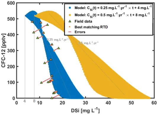
relationship between CFCs and DSi, Figure 5 shows the concentrations of CFC-12 and DSi 308

that can be reached with Inverse Gaussian RTDs, whatever their mean and standard 309

deviations in the range of 0-100 years for the two silicate weathering rates, i.e. 310 ) L mg 4 , yr L mg 0.25

(α = -1 -1 C_Si0 = -1 and (α =0.5mgL-1yr-1,C_Si0 =8mgL-1). Each point 311

represents an Inverse Gaussian RTD with specific parameters. Sampling well data of the 312

agricultural catchment 1 are shown as green triangles on the same plot for illustrative 313

purposes and the best RTD associated for each well sampled is represented among the 314

different Inverse Gaussian RTD by orange circles. The lower weathering scenario 315 ) L mg 4 , yr L mg 0.25

(α = -1 -1 C_Si0 = -1 explained much of the variability observed in the CFC-12 316

and DSi concentrations, suggesting that it is closer to the in situ rate. The difference between 317

the two envelopes underlines the high sensitivity of the weathering model and gives some 318

preliminary illustration of the capacity of extracting meaningful weathering properties. 319

(20)

19 320

Figure 4: CFC-12 vs DSi concentrations obtained for each of the field sites.

321

4.2 Catchment-based optimal weathering rates

322

We applied the same optimization method for each of the 5 catchments. ρ (the average 323

model error) varied significantly among catchments, with relatively small values (below 0.25) 324

for most of the catchments, but higher values for the pumped catchment (ρ =1.64; Table 2). 325

Optimal weathering rates were relatively similar among catchments, especially for the 326

agricultural catchments, which ranged from 0.20 to 0.23 mg L-1yr-1 (CV = 7%), demonstrating 327

regional consistency among different rock types. The weathering rate was significantly slower 328

(0.12 mg L yr-1) in the mountainous catchment and significantly faster in the pumped 329

catchment (0.31 mg L yr-1). 330

(21)

20 331

Figure 5: Calibration methodology. For each dataset representative of one site (Field data), the equation of

332

weathering (1) is optimized by minimizing the sum of the square errors between the well data and their best

333

matching Inverse Gaussian RTD in the RTD model ensemble. Two models ensemble are represented: the

334

blue one with (α,C_Si0 )= (0.25 mg L-1 yr-1, 4 mg L-1) and the yellow one with (α,C_Si0 )= (0.5 mg L-1 yr-1,

335

8 mg L-1). Notice how C_Si0 controls the horizontal position of the RTDs models in the (CFC, DSi) plot,

336

especially for the young fraction of the RTDs (high CFC-12, low DSi) while α controls the overall DSi

337

spreading of the models ensemble, especially for the old fraction of the RTDs (low CFC-12, high DSi).

338

Optimal initial DSi concentrations(C_Si0 )displayed some variability with a coefficient of 339

variation of 19% among catchments. On the extremes, the mountainous catchment showed an 340

initial DSi of 2.9 mg L-1 while the pumped catchment had an initial concentration of 341

5.0 mg L- 1, likely due to differences in weathering in the unsaturated zone. 342

Catchment ρ[-] α [mg L-1 yr-1] 0 Si

C [mg L-1] mean (µ) [yr] mean (σ ) [yr]

(22)

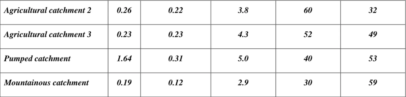
DSi as a groundwater dating proxy 13 April 2018 21 Agricultural catchment 2 0.26 0.22 3.8 60 32 Agricultural catchment 3 0.23 0.23 4.3 52 49 Pumped catchment 1.64 0.31 5.0 40 53 Mountainous catchment 0.19 0.12 2.9 30 59

Table 2: Results obtained from the calibration. ρis the residual (see equation (1)). α is the weathering

343

rate in mg L-1 yr-1, C_Si0, the initial DSi concentration in mg L-1. The two last columns present some

344

statistics about the parameters of the inverse Gaussian distributions optimized for each well: the average of

345

the mean residence time µ in years and the average of the standard deviation σ in years of the residence

346

time distributions for each catchment.

347

4.3 Models of RTDs

348

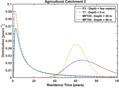
The largest differences between well-level RTDs occurred in the agricultural catchment 349

2 (Figure 6). The wells intersecting deep productive fractures had high DSi concentration and 350

low CFC concentrations (Figure 4) and displayed broad RTDs between 40 and 100 years 351

(Table 2 and yellow and purple curves in Figure 6). The low CFC concentrations 352

corresponded with the modeled RTDs, which indicated limited modern water (less than 15 to 353

20 years’ old). High DSi concentration requires much longer timescales and can be modeled 354

as well by the contribution of residence times above 40 years. The water residence time 355

distributions of the shallow wells (blue and red curves of Figure 6) showed significantly 356

younger water due to the lack of the old water contributions coming from deeper fractures 357

(Figure 6). 358

(23)

22 359

Figure 6: Illustration of the calibrated Inverse Gaussian RTD obtained on the agricultural catchment 2

360

(Saint Brice). The wells lying in the shallowest part of the aquifers have small residence times and

361

exponential shapes. The wells lying in the deepest part of the aquifer display some skewed distributions.

362

To get an idea of the type of RTDs obtained for the other catchments, we also compared 363

some statistics of the RTDs between sites, obtained with the optimization reported in Table 2. 364

All catchments have RTDs with mean residence times, which range on average between 30 365

years for the mountainous catchment and 60 years for the agricultural catchment 2. 366

4.4 Relations between DSi and mean residence times

367

A byproduct of the calibration of the inverse Gaussian lumped parameter model for the 368

DSi and CFC concentrations was the relation between the modeled mean residence times and 369

the observed DSi concentrations here shown for the three agricultural catchments located in 370

Brittany (Figure 7). For each catchment, the relation appeared to be linear, reinforcing the 371

consistency between the observed and modeled concentrations, and providing support for the 372

assumptions of the modeling approach. More specifically, the direct proportionality of the 373

DSi concentration to the mean residence time validated weathering assumptions modeled by a 374

(24)

23

zero-order kinetic reaction (equation (1)). The linear relations were also similar among 375

catchments with coefficients of variation of respectively 7% and 6%, for the different 376

weathering rates and the initial DSi concentration of the agricultural catchments. 377

378

Figure 7: Measured DSi concentration versus the optimized mean residence time of the inverse Gaussian

379

lumped distribution for three of the Brittany sites. Straight lines represent the optimized weathering law for

380

each of the sites. Note that it fits the measurements. Considering a constant weathering rate allows direct

381

interpretation of DSi apparent ages into mean residence times.

382

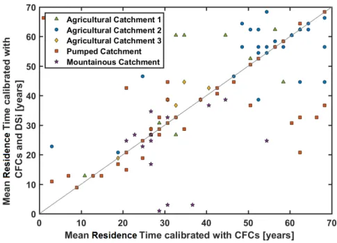
We compared these modeled mean residence times obtained with the CFC and DSi 383

concentrations with the mean residence times calibrated only with the CFC concentrations 384

(Figure 8). These CFC-only mean residence times were obtained using equation (1) without 385

considering DSi concentrations. For each of the wells in the different catchments, the mean 386

residence times obtained were quite consistent, especially for mean residence times ranging 387

between 0 and 50 years. For such a time range, a linear regression gives 𝜇_{𝐷𝑆𝑖−𝐶𝐹𝐶𝑠} = 388

1.03 𝜇𝐶𝐹𝐶𝑠 with a R2 of 0.36.

(25)

24 390

Figure 8: Comparison between the mean residence time obtained with CFCs and DSi concentrations with

391

those obtained only with the CFC concentrations.

392

5 Discussion

393

While DSi has been used as a site-specific indicator of groundwater residence time 394

(Burns et al., 2003; Kenoyer and Bowser, 1992; Morgenstern et al., 2010; Peters et al., 2014), 395

it was unknown how consistent silica weathering rates were, and consequently if DSi could be 396

a useful tracer at regional scales. In this study, we evaluated the use of DSi for groundwater 397

dating at four catchments in Brittany and one catchment in the Vosges Mountains. The data 398

and our simulations supported the hypothesis that silica weathering can be described by a 399

zero-order kinetic reaction at the catchment scale, and we calibrated silicate weathering laws 400

using CFC atmospheric tracers. We found that DSi provided complementary information to 401

CFC atmospheric tracers on RTDs. The relative stability of weathering rates among the 402

Brittany agricultural catchments validates the use of DSi as a regional groundwater age proxy. 403

We discuss below how these weathering rates may be modified by climatic context (from the 404

oceanic conditions of Brittany to the mountainous climate of the Vosges) and by external 405

(26)

25

factors, e.g. groundwater abstraction. Finally, we discuss the use of DSi for evaluating 406

residence times in unsaturated zones and compare these optimized silicate weathering rates to 407

weathering rates estimated in previous studies. 408

5.1 Practical use of DSi as a proxy of groundwater residence time

409

DSi concentration appears to be a highly complementary tracer to atmospheric tracers 410

such as CFCs. For example, at the agricultural catchment 2 (Figure 6), the comparison of 411

wells of different depths (shallow wells for P3 and T7, and deeper wells for MFT 20 and 412

MFT80) revealed that DSi concentration can infer the RTD even when CFCs are not 413

discriminating because they are below their detection limit for older ages (> 70 years) or 414

during the flat portion of their atmospheric trend (i.e. the last 0-20 years). These time ranges 415

where CFCs are less informative are further exacerbated by the widening of the concentration 416

area reachable by the inverse Gaussian function towards lower and higher CFC-12 417

concentration (Figure 5). For such CFC range (for example, for CFC-12 between 450 and 418

550 pptv and between 0 and 50 pptv), DSi is particularly useful to better characterize RTD. 419

The comparison between the modeled mean residence times and those calibrated only with 420

CFCs (Figure 8) also displayed an increased consistency for the time range between 0 and 50 421

years. For mean residence times above 50 years, DSi appears to give complementary 422

information to mean residence times from CFCs as depicted by the increased variability of 423

mean residence times around the identity line 𝑦 = 𝑥. 424

The bulk linear relation for weathering rate (equation (1)) is also of interest for dating 425

purposes as DSi concentrations can be seen as a direct proxy of the mean residence time 426

(Figure 7), which is not the case for other tracers such as CFCs (Figure 1) (Leray et al., 2012; 427

Marçais et al., 2015; Suckow, 2014). While this result has been obtained with a specific 428

Lumped Parameter Model (inverse Gaussian), it is generally applicable for a broad range of 429

(27)

26

distributions as it relies on the zero-order weathering assumption that leads to a linear 430

dependence of the DSi concentration on residence times (equation (1)). 431

Even if the small residuals obtained in Table 2 indicate that the inverse Gaussian model 432

may be appropriate for RTDs, other types of distributions, like the Gamma distribution, can 433

be tested to assess the sensitivity of the LPM choice to the RTD-related prediction. For the 434

agricultural catchment 1 and the pumped catchment, shapes of the Inverse Gaussian LPM as 435

well as the statistics obtained regarding the optimized RTDs (Table 2) are consistent with 436

results obtained synthetically from calibrated 3D flow and transport models developed for 437

these aquifers (Kolbe et al., 2016; Leray et al., 2012). 438

The 5 to 100 years’ time range of the RTDs observed here is the most favorable case for 439

using DSi for groundwater dating since it leads to thermodynamic-limitation conditions which 440

sustains chemical weathering (Maher, 2010). Even though weathering rates α might be quite 441

variable between different crystalline rock types, the fluid-rock contact time controls the 442

evolution of DSi concentrations for residence times ranging from years to decades (5-100 443

years) where dissolution is the dominant process. On the contrary, attainment of the mineral 444

equilibrium restricts the use of DSi for estimating longer residence times (>300 years) when 445

dissolution is balanced by re-precipitation (Edmunds and Smedley, 2000). 446

5.2 Stability of silica weathering rates at the regional scale

447

5.2.1 DSi as a robust regional groundwater age proxy 448

Our results indicate that DSi can be used as groundwater age tracing tool in relatively 449

diverse geologic contexts, as indicated by the consistency of the weathering rates for the 450

different Brittany catchments (Figure 7). This homogeneity suggests that only a few mineral 451

phases are responsible for silica production in the studied residence-time range; typically 452

phyllosilicates, plagioclase, and accessory minerals such as apatite are the major sources of 453

(28)

27

silica (Aubert et al., 2001). Applying a uniform weathering rate (0.22 mg L-1 yr-1) and initial 454

DSi concentration (4.0 mg L-1) can provide a first order estimate of mean residence time, as 455

displayed by the blue curve presented in Figure 9 compared to the weathering rates of each of 456

the Brittany catchments displayed in Figure 7. The relatively small error associated with 457

catchment specific differences justifies the possible use of DSi as a regional groundwater 458

dating tracer, as long as a weathering law can be applied based on similar catchments or land 459

lithologies. If more complete modeling is available, the choice between weathering laws can 460

be bypassed by directly solving the mass balance of the geochemical water content (Burns et 461

al., 2003). 462

463

Figure 9: DSi concentrations versus the optimized mean residence time of the inverse Gaussian displayed

464

for each wells for the mountainous and the pumped catchment. Straight lines represent the optimized

465

weathering law for each of the sites. Note that it fits the measurements. Considering a constant weathering

466

rate enables to indistinctly consider Si apparent ages and mean residence times.

467

Silicates are ubiquitous in most geological matrices, including crystalline and 468

sedimentary rocks (Iler, 1979). There is some evidence for using DSi as a groundwater age 469

(29)

28

proxy in other rock types (e.g. sedimentary rocks coming from glacial deposits, see section 470

5.4) (Becker, 2013; Kenoyer and Bowser, 1992). DSi concentration is widely measured and 471

accessible through public observatories and databases (Abbott et al., 2018; De Dreuzy et al., 472

2006; Thomas et al., 2016b). While previous studies have shown dependency of weathering 473

rates on lithology and climate (White and Blum, 1995; White et al., 1999; White et al., 2001), 474

DSi might be considered a “contextual tracer”, allowing at least local and potentially regional 475

groundwater dating (Beyer et al., 2016). 476

A major advantage of DSi is that it persists in open surface waters (e.g. lakes and 477

streams), whereas other tracers of intermediate transit times such as 3H/He and CFCs quickly 478

equilibrate with the atmosphere. Additionally, because artificial sources are few and 479

background concentration is usually high, DSi is robust to contamination, unlike CFCs, which 480

cannot be in contact with the atmosphere during sampling nor with any plastic surfaces 481

(Labasque et al., 2014). However, uptake of DSi by some vegetation and diatoms could 482

potentially limit the use of DSi in some environments especially during the growing season 483

(beginning of summer) (Delvaux et al., 2013; Pfister et al., 2017). This uptake is more likely 484

in large rivers systems where DSi spend enough time to be effectively captured by diatoms 485

whereas it is less prone to occur in headwaters systems with much smaller stream residence 486

times (Hughes et al., 2013). To track this potential additional process into account, diatom 487

uptake could be modeled (Thamatrakoln and Hildebrand, 2008) and/or isotopic DSi ratios 488

could be investigated to link in stream DSi concentration to mean transit time (Delvaux et al., 489

2013). 490

5.2.2 Comparison between the agricultural catchments and the mountainous catchment 491

Weathering rates were relatively constant within a given regional geological and climatic 492

context (e.g. for the three catchments in Brittany), but they were significantly different from 493

(30)

29

the mountainous catchment (Vosges Mountains). Differences in lithology could control 494

overall weathering rates, but this was not supported by the observed homogeneity of the 495

weathering rate across different lithologies (section 5.2.1). Acidity could not either explain 496

this variability, as pH was comparable for all the catchments (Table 1). The lower rates in the 497

mountainous catchment may be due to a difference in climatic conditions (i.e. temperature 498

and rainfall) between Brittany and the Vosges Mountain (Table 1). The ~3 factor difference 499

between DSi in the Vosges and Brittany could be explained by the combined effect of the 500

groundwater temperature difference (~6°C) and precipitation difference (~1.5-fold). Indeed, 501

temperature affects weathering rates by one order of magnitude from 0 to 25°C (White and 502

Blum, 1995; White et al., 1999). This increase is further emphasized by increasing recharge 503

fluxes, which is related to rainfall conditions. Another effect which could explain the 504

difference for the mountainous catchment is lack of anthropogenic pressure related to 505

agriculture. Brittany is a region of intensive agriculture characterized by high nitrogen loads, 506

which induce soil acidification. High weathering rates have been observed related to fertilized 507

additions (Aquilina et al., 2012a) which may also partially explain the Vosges-Brittany 508

difference. Anyway, climatic and anthropogenic influences are not exclusive and may be 509

combined to explain the high weathering rate difference. 510

5.2.3 Effect of groundwater abstraction on the weathering rate 511

The weathering law for heavily-pumped catchment in Plœmeur (orange line, Figure 9) 512

displayed a substantially higher weathering rate (0.31 mg L-1 yr-1) compared to the average 513

Brittany weathering rate (0.22 mg L-1 yr-1). This might be due to the presence of CFC 514

contamination leading to artificially enriched CFC concentrations compared to their actual 515

residence times. The pumped catchment is indeed especially vulnerable to CFC 516

contaminations (Table 1). However, long-term monitoring of CFC and SF6 and 3H/3He

517

measurements in this site makes the contamination hypothesis unlikely (Tarits et al., 2006). 518

(31)

30

The difference is more likely explained by the facts that: i) high and long-term pumping has 519

mobilized older waters (>100 years), which increase DSi concentrations without substantially 520

altering CFC concentrations (only dilution effect) (Figure 4); ii) pumping leads to a renewal 521

of groundwater flow paths with more reactive surfaces, leading to an increase of the reactive 522

surface/groundwater ratio. 523

5.3 Use of DSi for inferring residence times in the unsaturated zone

524

We hypothesized that the differences in initial DSi concentration are due to residence 525

time in the unsaturated zone, suggesting that DSi concentration at the groundwater table 526

surface (or modeled intercepts) could be used to infer residence times in the unsaturated zone. 527

Indeed the variability in C observed in Table 2 is correlated with the average unsaturated _Si0 528

zone thickness (Table 1), a major, though not exclusive, control on the time spent in the 529

unsaturated zone (Figure 10). The high C for the pumped catchment (5.0 mg L_Si0 -1) could be 530

due to pumping-induced drawdown of the water table, which significantly increases the 531

unsaturated zone thickness. Likewise, the mountainous catchment has a much shallower water 532

table depth, which might be related to the low initial DSi concentration (2.9 mg L-1). DSi 533

could therefore be a tracer of the full residence time in both unsaturated and saturated zones. 534

Yet, unless weathering rates in the unsaturated zone can be constrained, DSi estimates would 535

remain qualitative. Through tracing experiments, Legout et al. (2007) estimated the residence 536

time in the mobile-compartment of the unsaturated zone of the Kerrien catchment (South 537

Brittany) as 2-3 m y-1, which induces weathering rates about 4 times higher than in the 538

saturated zone. However, the ratio mobile/immobile water is unknown but may represent a 539

large fraction of groundwater with long residence-time that may contribute to high DSi. 540

Because the unsaturated zone, including the base of the soil profile, is often the site of 541

elevated rates of biogeochemical activity (e.g. nitrogen retention and removal) (Legout et al., 542

(32)

31

2005) or storage, constraining the residence time of water and solutes in this zone would 543

allow better estimation of catchment and regional-scale resilience to nutrient loading and 544

overall ecological functioning (Abbott et al., 2016; Meter et al., 2016; Pinay et al., 2015). 545

546

Figure 10: Initial DSi concentrations versus the average unsaturated zone thickness. The average

547

unsaturated zone thickness of the agricultural catchment 1 was not available.

548

5.4 Comparison of weathering rates to previously estimated weathering rates

549

We compared the weathering rates obtained in this study with previously published 550

studies (Table 3). The catchments considered in these studies have crystalline or sedimentary 551

bedrocks derived from the erosion of crystalline formations. Apparent weathering rates have 552

been estimated by different methods, either by implementing the geochemical evolution of 553

groundwater through advanced reactive transport modeling (Burns et al., 2003; Rademacher 554

et al., 2001) or by directly comparing DSi concentrations with apparent ages derived from 555

atmospheric tracer data (Bohlke and Denver, 1995; Clune and Denver, 2012; Denver et al., 556

2010). Our methodology is intermediary as it combines lumped residence time distributions 557

with apparent weathering rates and inlet concentrations (atmospheric chronicles for CFCs and 558

initial concentration C for DSi). _Si0 559

(33)

32

Except for the data reported in Kenoyer and Bowser (1992), which consists of young 560

groundwater (0-4 yrs), all DSi weathering rates referred in Table 3 are within one order of 561

magnitude (0.1 to 1 mg L-1 yr-1). For catchments with apparent ages between 10 and 50 years, 562

weathering rates are clustered between 0.2 and 0.4 mg L-1 yr-1 (Figure 11), which is consistent 563

with weathering rates estimated in this study. 564

The initial decrease of weathering rates with the typical apparent ages might suggest a 565

power law dependence of weathering rates on groundwater age (Figure 11). However, for 566

older apparent ages, the weathering rates might also stabilize around 20 years (Figure 11, 567

insert) suggesting a transition from transport-limited to thermodynamically-limited conditions 568

consistent with what has been observed for feldspar minerals (Maher, 2010) with a slightly 569

older transition time (20 years here instead of 10 years). It will require more studies on this 570

residence time range (0-100 yrs) to decide between these two competing hypotheses (power 571

law dependence versus stabilization) and precisely locate the transition time (Ackerer et al., 572

2018). This could be investigated by systematically combining weathering studies with 573

groundwater age tracer analysis in a diversity of environmental observatories. If predictable 574

rates are not found, the use of a constant weathering rate (equation (1)) could be refined by 575

considering a first order kinetic reaction, although it would require the inference of an 576

additional parameter to describe weathering. 577

(34)

33 579

Figure 11: Silicate weathering rates α against the typical apparent age range Â from which they have been

580

obtained, in this study and in previous studies (insert: log-log representation, p-value of 2 10-5 obtained for

581

the fit).

(35)

34 583

Catchment α [mg L-1

yr-1] Geological Context Apparent

Age range Complementary information References

Chesterville Branch 0.34 Permeable sand and gravel units of the fluvial Pensauken Formation and

the marine glauconitic Aquia Formation. 5 – 40 yrs Part of Locust Grove Catchment (Bohlke and Denver, 1995) Morgan Creek Drainage 0.37 Permeable sand and gravel units of the fluvial Pensauken Formation and

the marine glauconitic Aquia Formation. 4 – 50 yrs Part of Locust Grove Catchment (Bohlke and Denver, 1995) Panola Mountain

Research Watershed 0.62

Panola Granite (granodiorite composition), a biotite–oligioclase– quartz–

microcline granite of Mississippian to Pennsylvanian age. 0 – 25 yrs Mainly Riparian Saprolite Aquifer (Burns et al., 2003) Bucks Branch

Watershed 0.91 Sediments of the Beaverdam Formation. 15 – 30 yrs

mainly fluvial and estuarine deposits of

sand, gravel, silt, and clays (Clune and Denver, 2012) Fairmount catchment 0.26 Permeable quartz sand and gravel of the Beaverdam Formation and

underlying sandy strata of the Bethany Formation. 5 – 35 yrs

well-drained settings with relatively deep

water tables and thick sandy aquifers (Denver et al., 2010) Locust Grove

catchment 0.16

Permeable quartz sand and gravel of the Pennsauken Formation underlain

by highly weathered glauconitic sands of the Aquia Formation. 5 – 50 yrs

well-drained settings with relatively deep

water tables and thick sandy aquifers (Denver et al., 2010) Lizzie Catchment 0.36 Several Pleistocene-age terrace deposits that are underlain by a confining

unit on the top of the Yorktown Formation. 5 – 50 yrs

predominantly poorly drained settings with

shallow water tables (Denver et al., 2010)

Willards Catchment 0.83

The lowermost unit of the system is the Beaverdam Sand, which is overlain by a 3 to 8 m thick layer of clay, silt, peat, and sand of the Omar Formation.

0 – 18 yrs predominantly poorly drained settings with

shallow water tables (Denver et al., 2010) Polecat Creek

Watershed 1.0

Piedmont crystalline coastal plain sediments and alluvium. Presence of

Saprolite. 0 – 30 yrs Bedrock garnet-biotite gneiss (Lindsey et al., 2003) Crystal Lake, Vilas

County (Wisconsin) 3.94 50 m of glacial sediment which overlies Precambrian bedrock. 0 – 4 yrs

Glacial sediments were eroded from

Precambrian bedrock lithologies (Kenoyer and Bowser, 1992) Sagehen Springs (CA). 0.17 – 1.11 Extensive glacial till deposits derived from a combination of andesite and

granodiorite basement rocks. The granodiorite consists primarily of plagioclase (40%), quartz (30%), hornblende (20%), and biotite (10%), and the andesite consists primarily of plagioclase (45%) with varying amounts of hornblende (5–25%) and augite (1–25%) and a small amount of glassy groundmass.

0 – 40 yrs Range of weathering rate determined for

each spring, only for plagioclase mineral. (Rademacher et al., 2001)

Sagehen Springs (CA). 0.06 - 0.35 0 – 40 yrs Range of weathering rate determined for

each spring, only for hornblende mineral. (Rademacher et al., 2001)

Lizzie Catchment 0.34 Several Pleistocene-age terrace deposits that are underlain by a confining

unit on the top of the Yorktown Formation. 5 – 50 yrs Unconfined aquifer. (Tesoriero et al., 2005)

Table 3: Published weathering rates in different catchments obtained either directly or by fitting DSi concentrations against apparent ages. The typical age range

584

gives the spread of the water age data obtained from the different sampled wells.

(36)

35

6 Conclusion

586

We investigated the relationship between DSi and groundwater age tracers (CFCs) in five 587

different crystalline catchments, including lowland, mountainous, and actively pumped 588

catchments. For each catchment, we quantified the weathering rate and the RTDs at multiple 589

wells using inverse Gaussian lumped parameter models calibrated with geochemical data. 590

Overall, the DSi was strongly related to the exposure time between rocks and recently 591

recharged groundwater (i.e. between 5 to 100 years). We found that DSi was highly 592

complementary to CFCs, allowing better quantification of RTDs, including in the unsaturated 593

zone and for water masses younger and older than the now rapidly closing CFC use’s 594

window. The consistency of DSi weathering rates in three Brittany catchments suggests that 595

DSi may be a robust and cheap groundwater age proxy at regional scales for catchments with 596

comparable geology and climate. We interpreted DSi accumulation differences in the Brittany 597

pumped site and the mountainous region, as a consequence of temperature differences and 598

alterations of flow from groundwater abstraction respectively. If the temperature sensitivity of 599

weathering can be constrained, this tracer could allow widespread determination of water 600

transit time at the catchment scale for the unsaturated zone, aquifer, and surface waters. 601

Acknowledgements

602

We acknowledge the ANR for its funding through the project Soilµ-3D under the n° 603

ANR-15-CE01-0006. Dataset was provided by the OZCAR Network (Ploemeur - 604

hydrogeological observatory H+ network; Strengbach - Observatoire Hydrogéochimique de 605

l’Environnement) and the Zone Atelier Armorique (Pleine Fougères). We thank M. Bouhnik-606

Le-Coz and V. Vergnaud for the chemical analysis. We also thank H. V. Gupta for 607

constructive discussions. 608